A differential Lyapunov framework
for contraction analysis

Abstract

Lyapunov’s second theorem is an essential tool for stability analysis of differential equations. The paper provides an analog theorem for incremental stability analysis by lifting the Lyapunov function to the tangent bundle. The Lyapunov function endows the state-space with a Finsler structure. Incremental stability is inferred from infinitesimal contraction of the Finsler metrics through integration along solutions curves.

I Introduction

At the core of Lyapunov stability theory is the realization that a pointwise geometric condition is sufficient to quantify how solutions of a differential equation approach a specific solution. The geometric condition checks that the Lyapunov function, a certain distance from a given point to the target solution, is doomed to decay along the solution stemming from that point. By integration, the pointwise decay of the Lyapunov function forces the asymptotic convergence to the target solution. The basic theorem of Lyapunov has led to many developments over the last century, that eventually make the body of textbooks on nonlinear systems theory and nonlinear control [21, 45, 16, 17]. Yet many questions of nonlinear systems theory call for an incremental version of the Lyapunov stability concept, in which the convergence to a specific target solution is replaced by the convergence or contraction between any pairs of solutions [3, 26]. Essentially, this stronger property means that solutions forget about their initial condition. Popular control applications include tracking and regulation [35, 32], observer design [2, 41], coordination, and synchronization [55], to cite a few. Those incremental stability questions are often reformulated as conventional stability questions for a suitable error system, the zero solution of the error system translating the convergence of two solutions to each other. This ad-hoc remedy may be successful in specific situations but it faces unpleasant obstacles that include both methodological issues – such as the issue of transforming a time-invariant problem into a time-variant one – and fundamental issues – such as the issue of defining a suitable error between trajectories –. Those limitations also apply to the Lyapunov characterizations of incremental stability that have appeared in the recent years, primarily in the important work of Angeli [3].

In a seminal paper [26], Lohmiller and Slotine advocate a different angle of attack for nonlinear stability analysis. Their paper brings the attention of the control community to the basic fact that the distance measuring the convergence of two trajectories to each other needs not be constructed explicitly. Instead, it can be the integral of an infinitesimal measure of contraction. In other words, the often intractable construction of a distance needed for a global analysis can be substituted by a local construction. At a fundamental level, this approach brings differential geometry to the rescue of Lyapunov theory. The contraction concept of Lohmiller and Slotine – sometimes called “convergence” in reference to an earlier concept of Demidovich [33] – has been successfully used in a number of applications in the recent years [2, 35, 39, 55]. Yet, its connections to Lyapunov theory have been scarse, preventing a vast body of system theoretic tools to be exploited in the framework of contraction theory.

The present paper aims at bridging Lyapunov theory and contraction theory by formulating a differential version of the fundamental second’s Lyapunov theorem. Assuming that the state-space is a differentiable manifold, the classical concept of Lyapunov function in the (manifold) state-space is lifted to the tangent bundle. We call this lifted Lyapunov function a Finsler-Lyapunov function because it endows the differentiable manifold with a Finsler structure, which is precisely what is needed to associate by integration a global distance (or Lyapunov function) to the local construction. We formulate a Lyapunov theorem that provides a sufficient pointwise geometric condition to quantify incremental stability, that is, how solutions of differential equations approach each other. The pointwise properties of the Finsler-Lyapunov function in the tangent space guarantees that a suitable (integrated) distance function decays along solutions, proving incremental stability.

There are a number of reasons that motivate the Finsler structure as the appropriate differential structure to study incremental stability. Primarily, it unifies the approach advocated by Slotine – which equips the state-space with a Riemannian structure – and alternative approaches to contraction, such as the recent approach by Russo, Di Bernardo, and Sontag [39, 50] based on a matrix measure for the local measure of contraction. Examples in the paper further suggest that the Finsler framework will allow to unify the application of contraction to physical systems – typically akin to the Riemannian framework of classical mechanics – and to conic applications – typically akin to (non-Riemannian) Finsler metrics – such as consensus problems or monotone systems encountered in biology.

A primary motivation to study contraction in a (differential) Lyapunov framework is to make the whole body of Lyapunov theory available to contraction analysis. This is a vast program, only illustrated in the present paper by the very first extension of Lyapunov theorem based on LaSalle’s invariance principle. Although we are not aware of a published invariance principle for contraction analysis, its formulation in the proposed differential framework is a straightforward extension of its classical formulation and we anticipate this mere extension to be as useful for incremental stability analysis as it is for classical Lyapunov stability analysis.

We also include in this paper an extension of the basic theorem to the weaker notion of horizontal contraction. Horizontal contraction is weaker than contraction in that the pointwise decay of the Finsler-Lyapunov function is verified only in a subspace – called the horizontal subspace – of the tangent space. Disregarding contraction in specific directions is a convenient way to take into account symmetry directions along which no contraction is expected. This weaker notion of contraction is adapted to many physical systems and to many applications where contraction theory has proven useful, such as tracking, observer design, or synchronization. Those applications involve one or several copies of a given system and only the contraction between the copies and the system trajectories is of interest.

The rest of the paper is organized as follows. The notation is summarized in Section II. Sections III, IV, V contain the core of the differential framework through the introduction of the main definitions, results, and related examples. A detailed comparison with the existing literature is proposed in Section VI. Finally, LaSalle’s invariance principle and horizontal contraction are presented in Sections VII and VIII, respectively. Conclusions follow.

II Notation and preliminaries

We present the differential framework on general manifolds by adopting the notation used in [1] and [11]. A ($d$-dimensional) manifold $\mathcal{M}$ is a couple $(\mathcal{M},\mathcal{A}^{+})$ where $\mathcal{M}$ is a set and $\mathcal{A}^{+}$ is a maximal atlas of $\mathcal{M}$ into ${\mathbb{R}}^{d}$, such that the topology induced by $\mathcal{A}^{+}$ is Hausdorff and second-countable. We denote the tangent space of $\mathcal{M}$ at $x\in\mathcal{M}$ by $T_{x}\mathcal{M}$, and the tangent bundle of $\mathcal{M}$ by $T\mathcal{M}=\bigcup_{x\in\mathcal{M}}\{x\}\times T_{x}\mathcal{M}$.

Given two smooth manifolds $\mathcal{M}_{1}$ and $\mathcal{M}_{2}$ of dimension $d_{1}$ and $d_{2}$ respectively, consider a function $F:\mathcal{M}_{1}\to\mathcal{M}_{2}$ and a point $x\in\mathcal{M}_{1}$, and consider two charts $\varphi_{1}:\mathcal{U}_{x}\subset\mathcal{M}_{1}\to{\mathbb{R}}^{d_{1}}$ and $\varphi_{2}:\mathcal{U}_{F(x)}\subset\mathcal{M}_{2}\to{\mathbb{R}}^{d_{2}}$ defined on neighborhoods of $x$ and $F(x)$. We say that $F$ is of class $C^{k}$, $k\in\mathbb{N}$, if the function $\hat{F}=\varphi_{2}\circ F\circ\varphi_{1}^{-1}:{\mathbb{R}}^{d_{1}}\to{\mathbb{R}}^{d_{2}}$ is of class $C^{k}$. We say that $F$ is smooth (i.e. of class $C^{\infty}$) if $\hat{F}$ is smooth. The differential of $F$ at $x$ is denoted by $DF(x)[\cdot]:T_{x}\mathcal{M}_{1}\!\to\!T_{F(x)}\mathcal{M}_{2}$. It maps each tangent vector $\delta x\in T_{x}\mathcal{M}_{1}$ to $DF(x)[\delta x]\in T_{F(x)}\mathcal{M}_{2}\,$.

Given a manifold $\mathcal{M}$ of dimension $d$, to each chart $\varphi:\mathcal{U}\subset\mathcal{M}\to{\mathbb{R}}^{d}$ there corresponds a natural chart for $T\mathcal{M}$ given by $(\varphi(\cdot),D\varphi(\cdot)[\cdot]):T\mathcal{U}\subset T\mathcal{M}\to{\mathbb{R}}^{d}\times{\mathbb{R}}^{d}$. In particular, for every $x\in\mathcal{M}$, let $E_{i}$ be the $i$-the vector of th canonical basis of ${\mathbb{R}}^{d}$, then $\{D\varphi^{-1}(\varphi(x))[E_{1}],\dots,D\varphi^{-1}(\varphi(x))[E_{d}]\}$ is the natural basis of $T_{x}\mathcal{M}$.

A curve $\gamma$ on a given manifold $\mathcal{M}$, is a mapping $\gamma:I\subset{\mathbb{R}}\to\mathcal{M}$. A regular curve satisfies $D\gamma(s)[1]\neq 0$ for each $s\in I$. For simplicity we sometime use $\dot{\gamma}(s)$ or $\frac{d\gamma(s)}{ds}$ to denote $D\gamma(s)[1]$. Following [16, Appendix A], given a $C^{1}$ and time varying vector field $f$ on the manifold $\mathcal{M}$, which assigns to each point $x\in\mathcal{M}$ a tangent vector $f(t,x)\in T_{x}\mathcal{M}$ at time $t$, a $C^{1}$ curve $\gamma:I\to\mathcal{M}$ is an integral curve of $f$ if $D\gamma(t)[1]=f(t,\gamma(t))$ for each $t\in I$. We say that a curve $\gamma:I\to\mathcal{M}$ is a solution to the differential equation $\dot{\gamma}=f(t,\gamma)$ on $\mathcal{M}$ if $\gamma$ is an integral curve of $f$.

Throughout the paper we adopt the following notation. $I_{n}$ denotes the identity matrix of dimension $n$. Given a vector $v$, $v^{T}$ denotes the transpose vector of $v$. The span of a set of vectors $\{v_{1},\dots,v_{n}\}$ is given by $\mathrm{Span}(\{v_{1},\dots,v_{n}\}):=\{v\,|\,\exists\lambda_{1},\dots\lambda_{n}\in{\mathbb{R}}\mbox{ s.t. }v=\sum_{i=1}^{n}\lambda_{i}v_{i}\}$. Given a constant $c\in{\mathbb{R}}$ we write ${\mathbb{R}}_{\geq c}$ to denote the subset of $[c,\infty)\subset{\mathbb{R}}$. A locally Lipschitz function $\alpha:{\mathbb{R}}_{\geq 0}\rightarrow{\mathbb{R}}_{\geq 0}$ is said to belong to class $\mathcal{K}$ if it is strictly increasing and $\alpha(0)=0$; it belongs to class $\mathcal{K}_{\infty}$ if, moreover, $\lim_{r\rightarrow+\infty}\alpha(r)=+\infty$. A function $\beta:{\mathbb{R}}_{\geq 0}\times{\mathbb{R}}_{\geq 0}\to{\mathbb{R}}_{\geq 0}$ is said to belong to class $\mathcal{KL}$ if (i) for each $t\geq 0$, $\beta(\cdot,t)$ is a $\mathcal{K}$ function, and (ii) for each $s\geq 0$, $\beta(s,\cdot)$ is nonincreasing and $\lim_{t\to\infty}\beta(s,t)=0$.

A distance (or metric) $d:\mathcal{M}\times\mathcal{M}\to{\mathbb{R}}_{\geq 0}$ on a manifold $\mathcal{M}$ is a positive function that satisfies $d(x,y)=0$ if and only if $x=y$, for each $x,y\in\mathcal{M}$ and $d(x,z)\leq d(x,y)+d(y,z)$ for each $x,y,z\in\mathcal{M}$. Throughout the paper we assume that $d$ is continuous with respect to the manifold topology. Given a set $\mathcal{S}\subset\mathcal{M}$ we say that $\mathcal{S}$ is bounded if $\sup_{x,y\in\mathcal{S}}d(x,y)<\infty$ for any given distance $d$ on $\mathcal{M}$. The distance between a set $\mathcal{S}$ and a point $x$ is given by ${d}(\mathcal{A},x):=\sup_{y\in\mathcal{A}}{d}(y,x)$. We say that a curve $\gamma:I\to\mathcal{M}$ is bounded if its range is bounded. Given two functions $f:\mathcal{Z}\to\mathcal{Y}$ and $g:\mathcal{X}\to\mathcal{Z}$, the composition $f\circ g$ assigns to each each $p\in\mathcal{X}$ the value $f\!\circ\!g(p)=f(g(p))\in\mathcal{Y}$. Given a function $f:{\mathbb{R}}^{n}\to{\mathbb{R}}^{m}$ where we denote the (matrix of) partial derivatives by $\frac{\partial f(x)}{\partial x}$ and we write $\frac{\partial f(x)}{\partial x}_{|x=y}$ for the partial derivatives computed at $y\in{\mathbb{R}^{n}}$.

III Incremental stability and contraction

Consider a manifold $\mathcal{M}$ and a differential equation

$$\dot{x}=f(t,x)$$ (1)

where $f$ is a $C^{1}$ vector field which maps each $(t,x)\in{\mathbb{R}}\times\mathcal{M}$ to a tangent vector $f(t,x)\in T_{x}\mathcal{M}$. We denote by $\psi_{t_{0}}(\cdot,x_{0})$ the solution to (1) from the initial condition $x_{0}\in\mathcal{M}$ at time $t_{0}$, that is, $\psi_{t_{0}}(t_{0},x_{0})=x_{0}$. Throughout the paper, following [50], we simplify the exposition by considering forward invariant and connected subsets $\mathcal{C}\subset\mathcal{M}$ for (1) such that $\psi_{t_{0}}(\cdot,x_{0})$ is forward complete for every $x_{0}\in\mathcal{C}$, that is, $\psi_{t_{0}}(t,x_{0})\in\mathcal{C}$ for each $t_{0}$ and each $t\geq t_{0}$. For simplicity of the exposition, we also assume that every two points in $\mathcal{C}$ can be connected by a smooth curve $\gamma:I\to\mathcal{C}$.

The following definition characterizes several notions of incremental stability:

Definition 1

Consider the differential equation (1) on a given manifold $\mathcal{M}$. Let $\mathcal{C}\subset\mathcal{M}$ be a forward invariant set and $d:\mathcal{M}\times\mathcal{M}\to{\mathbb{R}}_{\geq 0}$ a continuous distance on $\mathcal{M}$. The system (1) is

(IS)

incrementally stable on $\mathcal{C}$ (with respect to $d$) if there exists a $\mathcal{K}$ function $\alpha$ such that $\forall x_{1},x_{2}\in\mathcal{C}$ , $\forall t_{0}\in{\mathbb{R}}$, $\forall t\geq t_{0}$,

$$d(\psi_{t_{0}}(t,x_{1}),\psi_{t_{0}}(t,x_{2}))\leq\alpha(d(x_{1},x_{2}))\ ;$$ (2)

(IAS)

incrementally asymptotically stable on $\mathcal{C}$ if it is incrementally stable and $\forall x_{1},x_{2}\in\mathcal{C}$, $\forall t_{0}\in{\mathbb{R}}$ ,

$$\lim\nolimits\limits_{t\to\infty}d(\psi_{t_{0}}(t,x_{1}),\psi_{t_{0}}(t,x_{2}))=0\;$$ (3)

(IES)

incrementally exponentially stable on $\mathcal{C}$ if there exist a distance $d$, $K\geq 1$, and $\lambda>0$ such that $\forall x_{1},x_{2}\in\mathcal{C}$, $\forall t_{0}\in{\mathbb{R}}$, $\forall t\geq t_{0}$,

$$d(\psi_{t_{0}}(t,x_{1}),\psi_{t_{0}}(t,x_{2}))\leq Ke^{-\lambda(t-t_{0})}d(x_{1},x_{2}).$$ (4)

$\lrcorner$

These definitions are incremental versions of classical notions of stability, asymptotic stability and exponential stability [21, Definition 4.4], and they reduce to those notions the metric space $(\mathcal{M},d)$ is complete and when either $x_{1}$ or $x_{2}$ is an equilibrium of (1). Global, regional, and local notions of stability are specified through the definition of the set $\mathcal{C}$. For example, we say that (1) is incrementally globally asymptotically stable when $\mathcal{C}=\mathcal{M}$. Note that both (IS) and (IES) properties are uniform with respect to $t_{0}$.

For $\mathcal{M}={\mathbb{R}^{n}}$ and for distances given by norms on ${\mathbb{R}^{n}}$, the notions of incremental stability and incremental asymptotic stability given above are equivalent to the notions of incremental stability and attractive incremental stability of [23, Definition 6.22], respectively. For $\mathcal{C}={\mathbb{R}^{n}}$, the notion of incremental asymptotic stability is weaker than the notion of incremental global asymptotic stability of [3, Definition 2.1], since the latter requires uniform attractivity.

Incremental stability of a dynamical system has been previously characterized by a suitable extension of Lyapunov theory [3]. For $\mathcal{M}={\mathbb{R}^{n}}$, the existence of a Lyapunov function decreasing along any pair of solutions is a sufficient condition for incremental stability [23, Theorem 6.30]. The key fact is in recognizing the equivalence between the incremental stability of $\dot{x}=f(t,x)$, $x\in{\mathbb{R}^{n}}$, and the stability of the set $\mathcal{A}:=\{(x_{1},x_{2})\in{\mathbb{R}}^{2n}\,|\,x_{1}=x_{2}\}$ for the extended system $\dot{x}_{1}=f(t,x_{1})$, $\dot{x}_{2}=f(t,x_{2})$. As a direct consequence, incremental asymptotic stability is inferred from the existence of a Lyapunov function $V(x_{1},x_{2}$) for the set $\mathcal{A}$ with (uniformly) negative derivative along the vector field $f(t,x_{1})$, $f(t,x_{2})$, for any pair $x_{1},x_{2}$. The extension to general manifolds is immediate.

IV Finsler-Lyapunov functions

This section introduces a concept of Lyapunov function in the tangent bundle $T\mathcal{M}$ of a manifold $\mathcal{M}$.

Definition 2

Consider a manifold $\mathcal{M}$. A $C^{1}$ function $V:T\mathcal{M}\to{\mathbb{R}}_{\geq 0}$ that maps every $(x,\delta x)\in T\mathcal{M}$ to $V(x,\delta x)\in{\mathbb{R}}_{\geq 0}$, is a candidate Finsler-Lyapunov function for (1) if there exist $c_{1},c_{2}\in{\mathbb{R}}_{\geq 0}$, $p\in{\mathbb{R}}_{\geq 1}$, and (a Finsler structure) $F:T\mathcal{M}\to{\mathbb{R}}_{\geq 0}$ such that, $\forall(x,\delta x)\in T\mathcal{M}$,

$$c_{1}F(x,\delta x)^{p}\leq V(x,\delta x)\leq c_{2}F(x,\delta x)^{p}.$$ (5)

$F$ satisfies the following conditions:

• $F$ is a $C^{1}$ function for each $(x,\delta x)\in T\mathcal{M}$ such that $\delta x\neq 0$;

• $F(x,\delta x)>0$ for each $(x,\delta x)\in T\mathcal{M}$ such that $\delta x\neq 0$;

• $F(x,\lambda\delta x)=\lambda F(x,\delta x)$ for each $\lambda\geq 0$ and each $(x,\delta x)\in T\mathcal{M}$ (homogeneity);

• $F(x,\delta x_{1}+\delta x_{2})<F(x,\delta x_{1})+F(x,\delta x_{2})$ for each $(x,\delta x_{1}),(x,\delta x_{2})\in T\mathcal{M}$ such that $\delta x_{1}\neq\lambda\delta x_{2}$ for any given $\lambda\in{\mathbb{R}}$ (strict convexity).

$\lrcorner$

For each $x\in\mathcal{M}$, $V$ is a measure of the length of the tangent vector $\delta x\in T_{x}\mathcal{M}$. The reason to call such a function $V$ a “Finsler-Lyapunov function” is that it combines the properties of a Lyapunov function and of a Finsler structure. The connection with classical Lyapunov functions is at methodological level: a candidate Finsler-Lyapunov function $V$ is an abstraction on the system tangent bundle $T\mathcal{M}$, used to characterize the asymptotic behavior of the system trajectories by looking directly at the vector field $f(t,x)$. Indeed, $V$ will be used as a Lyapunov function for the variational system associated to (1). (5), combined to the fact that $F(x,\cdot)$ defines an asymmetric norm $|\cdot|_{x}:=F(x,\cdot)$ in each tangent space $T_{x}\mathcal{M}$, emphasizes the analogies between Finsler-Lyapunov functions and classical Lyapunov functions. Note that the continuous differentiability of $V$ can be relaxed as in classical Lyapunov theory, see Remark 2 below. In a similar way, the restriction to time-invariant functions $V$ is only for notational convenience but all the results of the paper extend in a straightforward manner to time-varying functions $V$ .

The connection with Finsler structures is provided by Items (i)-(iv), which make $F$ a Finsler structure on $\mathcal{M}$ [52]. Positiveness, homogeneity, and strict convexity of $F$ guarantee that $F(x,\cdot)$ is a (possibly asymmetric) Minkowski norm in each tangent space. Thus, the length of any curve $\gamma$ induced by $F$ is independent on orientation-preserving reparameterizations of $\gamma$.

The relation (5) between a candidate Finsler-Lyapunov function $V$ and the associated Finsler structure $F$ is a key property for the deduction of incremental stability. This is because $F$ induces a well-defined distance on $\mathcal{M}$ via integration. Following [6, p.145],

Definition 3

[Finsler distance] Consider a candidate Finsler-Lyapunov function $V$ on the manifold $\mathcal{M}$ and the associated Finsler structure $F$ in Definition 2. For any subset $\mathcal{C}\subset\mathcal{M}$ and any two points $x_{1},x_{2}\in\mathcal{M}$, let $\Gamma(x_{1},x_{2})$ be the collection of piecewise $C^{1}$ curves $\gamma:I\to\mathcal{C}$, $I:=\{s\in{\mathbb{R}}\,|\,0\leq s\leq 1\}$, $\gamma(0)=x_{1}$, and $\gamma(1)=x_{2}$.

The distance (or metric) $d:\mathcal{M}\times\mathcal{M}\to{\mathbb{R}}_{\geq 0}$ induced by $F$ satisfies

$$d(x_{1},x_{2}):=\inf_{\Gamma(x_{1},x_{2})}\int_{I}F(\gamma(s),\dot{\gamma}(s))ds.\vspace{-5mm}$$ (6)

$\lrcorner$

We consider curves whose domain is restricted to $0\leq s\leq 1$ because any distance induced by $F$ is independent from any orientation-preserving reparameterization of curves. With a slight abuse of notation, in (6) we write $\dot{\gamma}(s)=D\gamma(s)[1]$ to denote the directional derivative of a given piecewise $C^{1}$ function $\gamma$ at $s$, implicitly assuming that the differential is computed only where the function is differentiable. Points of non-differentiability characterize a set of measure zero, which can be neglected at integration.

Example 1

We review specific classes of candidate Finsler-Lyapunov functions and classical distance functions. Consider $\mathcal{C}=\mathcal{M}={\mathbb{R}^{n}}$ (for simplicity) and consider the Riemannian structure $\langle\delta x_{1},\delta x_{2}\rangle_{x}:=\delta x_{1}^{T}P(x)\delta x_{2}$ for each $x\in\mathcal{M}$ and each $\delta x_{1},\delta x_{2}\in T_{x}\mathcal{M}$, where $P(x)$ is a symmetric and positive definite matrix in ${\mathbb{R}}^{n\times n}$ for each $x\in\mathcal{M}$. Then, the function $V:T\mathcal{M}\to{\mathbb{R}}_{\geq 0}$ given by $V(x,\delta x):=\langle\delta x,\delta x\rangle_{x}$ satisfies the conditions of Definition 2. Moreover, from Definition 3, the distance induced by $F=\sqrt{V}$ is given by the length of the geodesic connecting $x_{1}$ and $x_{2}$.

For the particular selection $P(x)=I$, $V(x,\delta x)$ reduces to $|\delta x|^{2}_{2}$. Thus, $d(x_{1},x_{2})=\int_{0}^{1}\left|\frac{\partial\gamma(s)}{\partial s}\right|_{2}ds$ where ${\gamma}$ is the straight line $\gamma(s):=(1-s)x_{1}+sx_{2}$. Therefore, $d(x_{1},x_{2})=\int_{0}^{1}|x_{2}-x_{1}|_{2}ds=|x_{1}-x_{2}|_{2}$. Note that for distances $d$ given by $k$-norms $d(x_{1},x_{2}):=|x_{1}-x_{2}|_{k}$, where $k\in\mathbb{N}$, $k\neq 2$, and $x_{1},x_{2}\in\mathcal{M}$, a quadratic Finsler-Lyapunov function $V$ (i.e. $F$ given by a Riemannian structure) is too restrictive. Nevertheless, taking $V(x,\delta x):=|\delta x|_{k}$, we have that $d(x_{1},x_{2})=|x_{1}-x_{2}|_{k}$.   $\lrcorner$

Example 2

We illustrate the importance of the relation (5) between Finsler-Lyapunov functions $V$ and Finsler structures $F$. As a first example, consider the manifold $\mathcal{M}={\mathbb{R}}^{2}$ and take $V(x,\delta x)=1$ for each $x\in{\mathbb{R}}^{2}$ and $\delta x\in{\mathbb{R}}^{2}$. Clearly, a function $F$ that satisfies Items (i)-(iv) in Definition 2 and (5) does not exist. However, mimicking (6), we could consider the following notion of “distance” based on $V$, $d(x_{1},x_{2}):=\inf_{\Gamma(x_{1},x_{2})}\int_{I}V(\gamma(s),\dot{\gamma}(s))ds$. Given any to points $x_{1},x_{2}\in\mathcal{M}$, consider a generic curve $\gamma:I\subset{\mathbb{R}}_{\geq 0}\to\mathcal{M}$, $I=[0,1]$, such that $\gamma(0)=x_{1}$ and $\gamma(1)=x_{2}$. Then, $\int_{I}V(\gamma(s),\dot{\gamma}(s))=\int_{I}1ds=1$. Consider now a reparameterization of $\gamma$ given by $\gamma_{k}:I_{k}\to\mathcal{M}$, $I_{k}=[0,\frac{1}{k}]$, such that $\gamma_{k}(0)=x_{1}$ and $\gamma_{k}(\frac{1}{k})=x_{2}$ for any $k>1$. By definition, we get that $d(x_{1},x_{2})\leq\lim\nolimits\limits_{k\to\infty}\int_{I_{k}}1ds=\lim\nolimits\limits_{k\to\infty}\frac{1}{k}=0$, for any given $x_{1},x_{2}\in\mathcal{M}$. Thus, $d$ is non-negative and satisfies the triangle inequality but $d(x_{1},x_{2})=0$ for $x_{1}\neq x_{2}$. Therefore, $d$ is not a distance. Note that a similar argument extends to $V(x,\delta x)=W(x)$ where $W(x)$ is a positive and continuously differentiable function.

As a second example, consider the simplified setting $\mathcal{M}={\mathbb{R}}$. Given the points $0$ and $1$, consider the curve $\gamma_{k}(s):[0,\frac{1}{k}]\to{\mathbb{R}}$ such that $\gamma_{k}(s)=ks$, $k\in\mathbb{N}_{\geq 1}$. The function $V(x,\delta x):=|\delta x|^{p_{1}}+|\delta x|^{p_{2}}$ is a candidate Finsler-Lyapunov function only if $p_{1}=p_{2}$, with Finsler structure $F$ given by $F(x,\delta x)=|\delta x|$. Otherwise, a function $F$ that satisfies (5) and the homogeneity property in (iii) does not exists. As above, integrating $V$ does not provide a distance. For instance, for any given $p$, and any given $p_{1}$ and $p_{2}$, we have that $\int_{0}^{\frac{1}{k}}V(\gamma_{k}(s),\dot{\gamma}_{k}(s))^{\frac{1}{p}}=\int_{0}^{\frac{1}{k}}\left(k^{p_{1}}+k^{p_{2}}\right)^{\frac{1}{p}}ds=\frac{1}{k}\left(k^{p_{1}}+k^{p_{2}}\right)^{\frac{1}{p}}$ which preserves a constant value for any given reparameterization $\gamma_{k}$ only when $p=p_{1}=p_{2}$.   $\lrcorner$

The reader will notice that the distance $d$ induced by the Finsler structure $F$ associated to a candidate Finsler-Lyapunov function (5) is not symmetric in general, that is, we may have $d(x,y)\neq d(y,x)$ for some $x,y\in\mathcal{M}$. To induce a symmetric distance, it is sufficient to strengthen (iii) in Definition 2 to (iii)_b $F(x,\lambda\delta x)=|\lambda|F(x,\delta x)$ for each $\lambda$, and each $(x,\delta x)\in T\mathcal{M}$ (absolute homogeneity, [52]). Note that adopting (iii)_b reduces the generality of the class of Finsler-Lyapunov functions excluding, for example, Randers metrics [6, Section 1.3].

V A Finsler-Lyapunov theorem
for contraction analysis

Consider a manifold $\mathcal{M}$ of dimension $d$. In what follows, we exploit the manifold structure of the tangent bundle $T\mathcal{M}$ to provide geometric conditions for contraction in local coordinates. Any given chart $\varphi:\mathcal{U}\subseteq\mathcal{M}\to{\mathbb{R}}^{d}$ induces a natural chart on $T\mathcal{U}\subseteq T\mathcal{M}$ (see Section II) that maps each point $(x,\delta x)\in T\mathcal{M}$ to its coordinate representation $(x_{\ell},\delta x_{\ell}):=(\varphi(x),D\varphi(x)[\delta x])\in{\mathbb{R}}^{d}\times{\mathbb{R}}^{d}$. In local coordinates (1) is represented by $\dot{x}_{\ell}=f_{\ell}(t,x_{\ell})$ where $f_{\ell}:{\mathbb{R}}^{d}\to{\mathbb{R}}^{d}$ is given by $f_{\ell}(t,x_{\ell})=D\varphi(x)[f(t,x)]$ at $x=\varphi^{-1}(x_{\ell})$. In a similar way, the chart representation $V_{\ell}(x_{\ell},\delta x_{\ell})$ of a Finsler-Lyapunov function $V$ is given by $V(x,\delta x)$ computed at $(x,\delta x)=(\varphi^{-1}(x_{\ell}),D\varphi^{-1}(x_{\ell})[\delta x_{\ell}])$. With a slight abuse of notation, in what follows we drop the subscript $\ell$.

Theorem 1

Consider the system (1) on a smooth manifold $\mathcal{M}$ with $f$ of class $C^{2}$, a connected and forward invariant set $\mathcal{C}$, and a function ${\alpha}:{\mathbb{R}}_{\geq 0}\to{\mathbb{R}}_{\geq 0}$. Let $V$ be a candidate Finsler-Lyapunov function such that, in coordinates,

$$\frac{\partial V(x,\delta x)}{\partial x}f(t,x)+\frac{\partial V(x,\delta x)}{\partial\delta x}\frac{\partial f(t,x)}{\partial x}\delta x\leq-{\alpha}(V(x,\delta x))$$ (7)

for each $t\in{\mathbb{R}}$, $x\in\mathcal{C}\subseteq\mathcal{M}$, and $\delta x\in T_{x}\mathcal{M}$. Then, (1) is

(IS)

incrementally stable on $\mathcal{C}$ if $\alpha(s)=0$ for each $s\geq 0$;

(IAS)

incrementally asymptotically stable on $\mathcal{C}$ if $\alpha$ is a $\mathcal{K}$ function;

(IES)

incrementally exponentially stable on $\mathcal{C}$ if $\alpha(s)=\lambda s>0$ for each $s>0$.

$\lrcorner$

We say that the system (1) contracts $V$ in $\mathcal{C}$ if (7) is satisfied for some function $\alpha$ of class $\mathcal{K}$. $V$ is called the contraction measure, and $\mathcal{C}$ the contraction region.

The conditions of the theorem for incremental stability are reminiscent of classical Lyapunov conditions for stability, asymptotic stability and exponential stability [21, Chapter 4], lifted to the tangent bundle $T\mathcal{M}$. In fact, (7) guarantees that $V$ decreases along the trajectories of the variational system (in coordinates) $\dot{x}=f(x)$, $\dot{\delta x}=\frac{\partial f(x)}{\partial x}\delta x$. The reader will notice that along any solution $\psi_{t_{0}}(t,x_{0})$ to (1), $\dot{\delta x}=\left[\frac{\partial f(x)}{\partial x}_{|x=\psi_{t_{0}}(t,x_{0})}\right]\delta x$ characterizes the linearization of (1) along its trajectories. Thus, exploiting the relation between $V$ and Finsler structure, the contraction of the structure along $\psi_{t_{0}}(t,x_{0})$ (locally - in each tangent space) guarantees, via integration, that the distance between any pair of solutions $\psi_{t_{0}}(t,x_{1})$ and $\psi_{t_{0}}(t,x_{2})$, $x_{1},x_{2}\in\mathcal{C}$, shrinks to zero as $t$ goes to infinity. A graphical illustration is provided in Fig. 1.

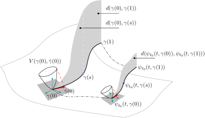
Figure 1: A graphical illustration of the contraction of the distance induced by Condition (7) on the solutions to (1). The Finsler-Lyapunov function assigns a positive value to each pair $(\gamma(s),\dot{\gamma}(s))$. The length of the curve $\gamma$ is given by the integral of the Finsler-Lyapunov function along $\gamma$, represented by the shaded area.

The incremental Lyapunov approach proposed in [3], establishes incremental stability by checking a pointwise geometric condition in the product space $\mathcal{M}\times\mathcal{M}$. In contrast, the differential approach proposed here establishes incremental stability by checking a pointwise geometric condition in the tangent bundle $T\mathcal{M}$. Several earlier works have adopted this approach in a Riemannian framework, focusing on quadratic functions $V(x,\delta x)=\delta x^{T}P(x)\delta x$ in Euclidean spaces (see Section VI). There are a number of reasons to consider Finsler generalizations of Riemannian structures for contraction analysis, some of which are illustrated in the next section, where we report a detailed comparison between the conditions proposed in Theorem 1 and several results available in literature.

Before entering into the details of the proof, we present a scalar example that illustrates the value of non-constant Riemannian structures in nonlinear spaces.

Example 3

For $\mathcal{M}=\mathbb{S}^{1}$ consider the dynamics

$$\dot{\vartheta}=f(\vartheta):=-\sin(\vartheta).$$ (8)

The tangent space at every point $\vartheta\in\mathcal{M}$ is given by ${\mathbb{R}}$. The naive choice $V_{1}(\vartheta,\delta\vartheta):=\frac{1}{2}\delta\vartheta^{2}$ corresponds to a constant Riemannian structure on $\mathcal{S}^{1}$. Then, for any given compact set $\mathcal{C}\subset(-\frac{\pi}{2},\frac{\pi}{2})$ (7) yields

$$\frac{\partial V_{1}(\vartheta,\delta\vartheta)}{\partial\delta\vartheta}\left(\frac{\partial f(\vartheta)}{\partial\vartheta}\right)\delta\vartheta=-\cos(\vartheta)\delta\vartheta^{2}<-\varepsilon V_{1}(\delta\vartheta)$$ (9)

where $\varepsilon>0$ (sufficiently small). From Theorem 1 we conclude that (8) is incrementally exponentially stable on compact sets $\mathcal{C}\subset(-\frac{\pi}{2},\frac{\pi}{2})$ such that $0\in\mathcal{C}$ (to guarantee that $\mathcal{C}$ is forward invariant). For $\mathcal{C}=[-\frac{\pi}{2},\frac{\pi}{2}]$ we have only incremental stability, since $\cos(\vartheta)=0$ at $|\vartheta|=\frac{\pi}{2}$. From Definition 3, note that the distance induced by $F=\sqrt{2V_{1}}$ is given by $|\vartheta_{1}-\vartheta_{2}|$.

A maximal contracting region is captured with the choice $V_{2}:(\mathbb{S}^{1}\setminus\{\pi\})\times{\mathbb{R}}\to{\mathbb{R}}_{\geq 0}$ given by $V_{2}=\frac{\delta\vartheta^{2}}{1+\cos{\vartheta}}$. Despite the identification of each $T_{\vartheta}\mathcal{M}$ with ${\mathbb{R}}$, the measure of the “length” of $\delta\vartheta$ given by $V_{2}$ now depends on $\vartheta$. Note that $V_{2}$ satisfies each condition of Definition 2 and is well defined in $\mathbb{S}^{1}\setminus\{\pi\}$ since $\frac{1}{1+\cos(\vartheta)}\to\infty$ as $|\vartheta|\to\pi$. For any given compact set $\mathcal{C}\subset(\mathbb{S}^{1}\setminus\{\pi\})$ such that $0\in\mathcal{C}$, (7) yields

$$\begin{array}[]{l}\frac{\partial V_{2}(\vartheta,\delta\vartheta)}{\partial\vartheta}f(\vartheta)+\frac{\partial V_{2}(\vartheta,\delta\vartheta)}{\partial\delta\vartheta}\left(\frac{\partial f(\vartheta)}{\partial\vartheta}\right)\delta\vartheta=\vspace{1mm}\\ \qquad=-\frac{\sin(\vartheta)^{2}}{(1+\cos(\vartheta))^{2}}\delta\vartheta^{2}-2\frac{\cos(\theta)}{1+\cos(\theta)}\delta\vartheta^{2}\vspace{2mm}\\ \qquad=-\frac{\sin(\vartheta)^{2}+2\cos(\vartheta)(1+\cos(\vartheta))}{(1+\cos(\vartheta))^{2}}\delta\vartheta^{2}\vspace{2mm}\\ \qquad=-\frac{1+2\cos(\vartheta)+\cos(\vartheta)^{2}}{(1+\cos(\vartheta))^{2}}\delta\vartheta^{2}\vspace{2mm}\\ \qquad=-\delta\vartheta^{2}\vspace{2mm}\\ \qquad\leq-\varepsilon V_{2}(\vartheta,\delta\vartheta),\end{array}$$ (10)

where $\varepsilon>0$. Thus, by Theorem 1, (8) is incrementally exponentially stable on $\mathcal{C}$.   $\lrcorner$

Proof of Theorem 1. The proof is divided in four main steps. For simplicity, we develop the calculations in coordinates.

(i) Setup: Finsler structure and parameterized solution.

For any two points $x_{1},x_{2}\in\mathcal{M}$, let $\Gamma(x_{1},x_{2})$ be the collection of piecewise $C^{1}$, equally oriented curves $\gamma:I\to\mathcal{C}\subset\mathcal{M}$, $I:=\{s\in{\mathbb{R}}\,|\,0\leq s\leq 1\}$, connecting $x_{1}$ to $x_{2}$, that is, $\gamma(0)=x_{1}$ and $\gamma(1)=x_{2}$. In coordinates, the distance $d$ induced by $F$ in Definition 3 reads

$$d(x_{1},x_{2})=\inf_{\Gamma(x_{1},x_{2})}\int_{I}F\left(\gamma(s),\frac{\partial\gamma(s)}{\partial s}\right)ds.$$ (11)

where $F$ is the associated Finsler structure to $V$ of Definition 2. For any two initial conditions $x_{1},x_{2}\in\mathcal{C}$ and any given $\varepsilon>0$, consider now a regular smooth curve $\overline{\gamma}:I\to\mathcal{C}\subset\mathcal{M}$ such that $\overline{\gamma}(0)=x_{1}$, $\overline{\gamma}(1)=x_{2}$, and

$$\int_{I}F\left(\overline{\gamma}(s),\frac{\partial\overline{\gamma}(s)}{\partial s}\right)ds\leq(1+\varepsilon)d(x_{1},x_{2}).$$ (12)

Let $\psi_{t_{0}}(\cdot,\overline{\gamma}(s))$ be the solution to (1) from the initial condition $\overline{\gamma}(s)$, for $s\in I$, at time $t_{0}$. Precisely, $\psi_{t_{0}}(\cdot,\overline{\gamma}(\cdot))$ is a function from ${\mathbb{R}}\times I$ to $\mathcal{M}$ that satisfies, in coordinates,

$$\frac{\partial}{\partial t}\psi_{t_{0}}(t,\overline{\gamma}(s))=f(t,\psi_{t_{0}}(t,\overline{\gamma}(s)))\quad\forall t\geq t_{0}\,,\ \forall\in I.$$ (13)

Clearly $\psi_{t_{0}}(t_{0},\overline{\gamma}(\cdot))=\overline{\gamma}(\cdot)$ thus, from (12), we have that

$$\int_{I}F\left(\psi_{t_{0}}(t_{0},\overline{\gamma}(s)),\frac{\partial}{\partial s}\psi_{t_{0}}(t_{0},\overline{\gamma}(s))\right)ds\leq(1+\varepsilon)d(x_{1},x_{2}).$$ (14)

As usual, for each $t\geq t_{0}$ and $s\in[0,1]$ the differential of $\psi$ in the direction $\frac{\partial}{\partial t}$ characterizes the time derivative of the parameterized solution $\psi_{t_{0}}(\cdot,\overline{\gamma}(s))$. Instead, the differential of $\psi$ in the direction $\frac{\partial}{\partial s}$ characterizes at each $s$ the tangent vector to the curve $\psi_{t_{0}}(t,\overline{\gamma}(\cdot))$, for fixed time $t$. Following [26], we call this tangent vector virtual displacement. Thus, combining integration of the displacement along $\frac{\partial}{\partial s}$, time derivative along $\frac{\partial}{\partial t}$, and (7), we can establish contraction of the distance (11) along the solutions to (1).

(ii) The displacement dynamics along the solution $\psi_{t_{0}}(\cdot,\overline{\gamma}(s))$.

Consider the function $\delta\psi_{t_{0}}(\cdot,\cdot):{\mathbb{R}}\times I\to T\mathcal{M}$ given by the tangent vector $\delta\psi_{t_{0}}(t,s):=D\psi_{t_{0}}(t,\overline{\gamma}(s))[0,1]$, which in coordinates is given by $\frac{\partial}{\partial s}\psi_{t_{0}}(t,\overline{\gamma}(s))$ for each $t\geq t_{0}$ and $s\in I$. Its time derivative is given by

$$\frac{\partial}{\partial t}\delta\psi_{t_{0}}(t,\overline{\gamma}(s)) = \frac{\partial^{2}}{\partial t\partial s}\psi_{t_{0}}(t,\overline{\gamma}(s))$$ (15a)

$$= \frac{\partial^{2}}{\partial s\partial t}\psi_{t_{0}}(t,\overline{\gamma}(s))$$ (15b)

$$= \frac{\partial}{\partial s}f(t,\psi_{t_{0}}(t,\overline{\gamma}(s)))$$ (15c)

$$= \left[\frac{\partial f(t,x)}{\partial x}\right]\frac{\partial}{\partial s}\psi_{t_{0}}(t,\overline{\gamma}(s))$$ (15d)

$$= \left[\frac{\partial f(t,x)}{\partial x}\right]\delta\psi_{t_{0}}(t,s).$$ (15e)

where $\frac{\partial f(t,x)}{\partial x}$ must be evaluated at $x=\psi_{t_{0}}(t,\overline{\gamma}(s))$. (15a) follows from the definition of $\delta\psi_{t_{0}}(t,s)$. (15b) follows from the fact that $\psi_{t_{0}}(\cdot,\overline{\gamma}(\cdot))$ is a $C^{2}$ function, since $f$ is a $C^{2}$ vector field and $\overline{\gamma}(\cdot)$ is a smooth curve [7, Theorem 4.1]. (15d) follows from the chain rule. Finally, (15e) follows from the definition of $\delta\psi_{t_{0}}(t,s)$.

(iii) The dynamics of $V$ along the solution $\psi_{t_{0}}(\cdot,\overline{\gamma}(s))$.

Consider the function $\overline{V}:{\mathbb{R}}\times I\to{\mathbb{R}}_{\geq 0}$ given by $\overline{V}(t,s)=V(\psi_{t_{0}}(t,\overline{\gamma}(s)),\delta\psi_{t_{0}}(t,s))$ for each $t\geq t_{0}$ and $s\in I$. Note that $\overline{V}$ has a well-defined time derivative $\frac{d}{dt}\overline{V}(t,s)$ since $\overline{V}(t,s)\in{\mathbb{R}}_{\geq 0}$ for each $t$ and $s$. In coordinates, for $x=\psi_{t_{0}}(t,\overline{\gamma}(s))$ and $\delta x=\delta\psi_{t_{0}}(t,s)$,

$$\frac{d}{dt}\overline{V}(t,s) = \left[\frac{\partial V(x,\delta x)}{\partial x}\right]\frac{\partial}{\partial t}\psi_{t_{0}}(t,\overline{\gamma}(s))+$$ (16b)

$$+\left[\frac{\partial V(x,\delta x)}{\partial\delta x}\right]\frac{\partial}{\partial t}\delta\psi_{t_{0}}(t,s)$$

$$= \left[\frac{\partial V(x,\delta x)}{\partial x}\right]f(t,\psi_{t_{0}}(t,\overline{\gamma}(s)))+$$

$$+\left[\frac{\partial V(x,\delta x)}{\partial\delta x}\right]\left[\frac{\partial f(t,x)}{\partial x}\right]\delta\psi_{t_{0}}(t,s)$$

$$\leq -\alpha(\overline{V}(t,s)).$$ (16c)

(16b) follows from the application of the chain rule. (16b) follows from (13) and (15). (16c) is enforced by (7).

(iv) Incremental stability properties. Consider the Finsler structure $F$ associated to the Finsler-Lyapunov function $V$. Define $\overline{F}:{\mathbb{R}}\times I\to{\mathbb{R}}_{\geq 0}$ as $\overline{F}(t,s)=F(\psi_{t_{0}}(t,\overline{\gamma}(s)),\delta\psi_{t_{0}}(t,s))$.

(IS) Incremental stability: if $\alpha(s)=0$ for each $s>0$ then

$$\overline{V}(t,s)\leq\overline{V}(t_{0},s)\quad\mbox{for all }t\geq t_{0}\mbox{ and }s\in I.$$ (17)

Therefore, for each $t\geq t_{0}$, exploiting (5) and (17), we get

$$\begin{array}[]{rcl}d(\psi_{t_{0}}(t,x_{1}),\psi_{t_{0}}(t,x_{2}))&\leq&\int_{I}\overline{F}(t,s)ds\\ &\leq&c_{1}^{-\frac{1}{p}}\int_{I}\overline{V}(t,s)^{\frac{1}{p}}ds\\ &\leq&c_{1}^{-\frac{1}{p}}\int_{I}\overline{V}(t_{0},s)^{\frac{1}{p}}ds\\ &\leq&(c_{2}/c_{1})^{\frac{1}{p}}\int_{I}\overline{F}(t_{0},s)ds\\ &\leq&(1+\varepsilon)(c_{2}/c_{1})^{\frac{1}{p}}d(x_{1},x_{2})\end{array}$$ (18)

where the first inequality follows from the definition of induced distance in (6), and the last inequality follows from (14).

(IAS) Incremental asymptotic stability: if $\alpha$ is a $\mathcal{K}$ function then $\frac{d}{dt}\overline{V}(t,s)\leq 0$, thus (IS) holds, moreover by [49, Lemma 6.1] and [15, Theorem 6.1], there exists a $\mathcal{KL}$ function $\beta$ such that

$$\overline{V}(t,s)\leq\beta(\overline{V}(t_{0},s),t-t_{0})\quad\mbox{for all }t\geq t_{0}\mbox{ and }s\in I.$$ (19)

Therefore, following the calculations in (18), for each $t\geq t_{0}$,

$$\begin{array}[]{rcl}d(\psi_{t_{0}}(t,x_{1}),\psi_{t_{0}}(t,x_{2}))&\leq&{c_{1}^{-\frac{1}{p}}}\int_{I}\overline{V}(t,s)^{\frac{1}{p}}ds\\ &\leq&{c_{1}^{-\frac{1}{p}}}\int_{I}\beta(\overline{V}(t_{0},s),t-t_{0})^{\frac{1}{p}}ds\end{array}$$ (20)

from which we get

$$\begin{array}[]{l}\lim\nolimits\limits_{t\to\infty}d(\psi_{t_{0}}(t,x_{1}),\psi_{t_{0}}(t,x_{2}))\\ \qquad\leq{c_{1}^{-\frac{1}{p}}}\lim\nolimits\limits_{t\to\infty}\int_{I}\beta(\overline{V}(t_{0},s),t-t_{0})^{\frac{1}{p}}ds\\ \qquad=0.\end{array}$$ (21)

The last identity is a consequence of the Lebesgue’s dominated convergence theorem, since $\beta(\overline{V}(t_{0},s),t-t_{0})$ is a monotonically decreasing function for $t\to\infty$.

(IES) Incremental exponential stability: if $\alpha(s)=\lambda s>0$ for each $s>0$ then, by [15, Theorem 6.1], we get

$$\overline{V}(t,s)\leq e^{-\lambda(t-t_{0})}\overline{V}(t_{0},s)\quad\mbox{for all }t\geq t_{0}\mbox{ and }s\in I.$$ (22)

Therefore, mimicking (18), for each $t\geq t_{0}$,

$$\begin{array}[]{l}d(\psi_{t_{0}}(t,x_{1}),\psi_{t_{0}}(t,x_{2}))\\ \qquad\leq{c_{1}^{-\frac{1}{p}}\int_{I}\overline{V}(t,s)^{\frac{1}{p}}ds}\\ \qquad\leq{c_{1}^{-\frac{1}{p}}e^{-\frac{\lambda}{p}(t-t_{0})}\int_{I}\overline{V}(t_{0},s)^{\frac{1}{p}}ds}\\ \qquad\leq{(c_{2}/c_{1})^{\frac{1}{p}}e^{-\frac{\lambda}{p}(t-t_{0})}\int_{I}\overline{F}(t_{0},s)ds}\\ \qquad\leq{(1+\varepsilon)(c_{2}/c_{1})^{\frac{1}{p}}e^{-\frac{\lambda}{p}(t-t_{0})}d(x_{1},x_{2}).}\end{array}\vspace{-5mm}$$ (23)

$\blacksquare$

The proof of Theorem 1 generalizes the argument proposed in the proof of [50, Lemma 1] and [39, Theorem 5] to general manifolds and Finsler structures (the proof provided in [39] is developed for Euclidean spaces using matrix measures). An equivalent proof to Theorem 1 for incremental exponential stability and $V$ restricted to Riemannian structures can be found in [2, Appendix II].

Remark 1

Consider the case $V(x,\delta x)=F(x,\delta x)^{p}$ in Definition 2. Then, from (12) and (18), for any given converging sequence $\varepsilon_{k}\in{\mathbb{R}}_{>0}$, $\lim\nolimits\limits_{k\to\infty}\varepsilon_{k}=0$, we can construct a sequence of $C^{2}$ curves $\gamma_{k}:I_{k}\to\mathcal{M}$ such that

$$\begin{array}[]{l}\lim\nolimits\limits_{k\to\infty}\int_{I_{k}}V(\gamma_{k}(s),D\gamma_{k}(s)[1])^{\frac{1}{p}}ds\\ \qquad\qquad\leq\lim_{k\to\infty}(1+\varepsilon_{k})d(x_{1},x_{2})\\ \qquad\qquad=d(x_{1},x_{2}).\end{array}$$ (24)

In such a case, in the limit of $k\to\infty$, (IS) in Theorem 1 guarantees incremental stability with the stronger property that

$$d(\psi_{t_{0}}(t,x_{1}),\psi_{t_{0}}(t,x_{2}))\leq d(x_{1},x_{2})\quad\forall t\geq t_{0},\forall x_{1},x_{2}\in\mathcal{M}.\vspace{-5mm}$$ (25)

$\lrcorner$

Remark 2

The result of Theorem 1 can be extended to piecewise continuously differentiable and locally Lipschitz candidate Finsler-Lyapunov functions $V$. In a similar way, the assumption that every two points of $\mathcal{C}$ are connected by a smooth curve $\gamma:I\to\mathcal{C}$ can be relaxed to piecewise smooth curves. The key observation is that the decrease of the distance between any two solutions is preserved also if (16) holds for almost every $t$ and $s$. With this aim, for example, let $\mathcal{D}\subseteq{T\mathcal{M}}$ be the set of nondifferentiable points of $V$. (16) holds for almost every $t$ and $s$ if for any given solution $\psi_{t_{0}}$ such that $(\psi_{t_{0}}(t,x),D\psi_{t_{0}}(t,x)[0,\delta x])\in\mathcal{D}$, there exists $\varepsilon>0$ which guarantees $(\psi_{t_{0}}(\tau,x),D\psi_{t_{0}}(\tau,x)[0,\delta x])\notin\mathcal{D}$ for every $\tau\in(t,t+\varepsilon]$. The transversality of the trajectories with respect to $\mathcal{D}$ can be enforced geometrically by requiring that, (in coordinates) for each $t\geq t_{0}$, and each $(x,\delta x)\in\mathcal{D}$, the pair $(f(t,x),\frac{\partial}{\partial x}f(t,x)\delta x)$ does not belong to the tangent cone to $\mathcal{D}$ at $(x,\delta x)$.   $\lrcorner$

We conclude the section by emphasizing the analogy between classical Lyapunov theory and Theorem 1. We also emphasize the geometric (or coordinate-free) nature of Theorem 1, showing that (7) in Theorem 1 is independent on the selected coordinate chart. With this aim, we introduce two charts $\varphi,\psi:\mathcal{U}\subseteq\mathcal{M}\to{\mathbb{R}}^{d}$, and we denote by $z$ and $y$ the coordinate representations $z=\varphi(x)$ and $y=\psi(x)$ of any point $x\in\mathcal{M}$. In particular, $V^{(z)}$ and $f^{(z)}(t,z)$ denote respectively the Finsler-Lyapunov function $V$ and the vector field (1) in the chart $\varphi$. $V^{(y)}$ and $f^{(y)}(t,y)$ denote the same quantities in the local chart $\psi$.

The analogy with classical Lyapunov theory is emphasized by considering the aggregate state $Z:=(z,\delta z)$. Suppose that (7) has been established by using the coordinate chart $\varphi$. Exploiting the notion of aggregate state, we define $\dot{Z}=f^{(Z)}(Z)$, where $f^{(Z)}(Z):=\left[\begin{smallmatrix}f^{(z)}(z)\\ \frac{\partial f^{(z)}(z)}{\partial z}\delta z\end{smallmatrix}\right]$, and $V^{(Z)}(Z):=V^{(z)}(z,\delta z)$, from which (7) reads $\frac{\partial V^{(Z)}(Z)}{\partial Z}f^{(Z)}(Z)\leq-\alpha(V^{(Z)}(Z)).$ This formulation reveals that the Finsler-Lyapunov approach is Lyapunov’s second method on the variational system. Clearly, a Finsler-Lyapunov function differs from classical Lyapunov functions, since its definition is tailored to endow $\mathcal{M}$ with the structure of a metric space.

Coordinate independence can be shown as follows. Define $Y:=(y,\delta y)$ and note that $Z=H(Y)$, where $H(y,\delta y):=(\varphi(\psi^{-1}(y)),\frac{\partial\varphi(\psi^{-1}(y))}{\partial y}\delta y)$. Necessarily, the vector field in the $Y$ coordinates reads $f^{(Y)}(Y)=\left[\frac{\partial H^{-1}(Z)}{\partial Z}_{|Z=H(Y)}\right]f^{(Z)}(H(Y))$, and $V^{(Y)}(Y)=V^{(Z)}(H(Y))$. Thus,

$$\begin{array}[]{rcl}\frac{\partial V^{(Y)}(Y)}{\partial Y}f^{(Y)}(Y)&=&\left[\frac{\partial V^{(Z)}(Z)}{\partial Z}_{|Z=H(Y)}\right]\cdot\vspace{1mm}\\ &&\cdot\underbrace{\frac{\partial H(Y)}{\partial Y}\left[\frac{\partial H^{-1}(Z)}{\partial Z}_{|Z=H(Y)}\right]}_{=I}\cdot\\ &&\cdot f^{(Z)}(H(Y))\vspace{1mm}\\ &=&\left[\frac{\partial V^{(Z)}(Z)}{\partial Z}_{|Z=H(Y)}\right]f^{(Z)}(H(Y))\vspace{1mm}\\ &\leq&-\alpha(V^{(Z)}(H(Y)))\vspace{1mm}\\ &=&-\alpha(V^{(Y)}(Y)),\\ \end{array}$$ (26)

which proves the coordinate independence of (7).

VI Revisiting some literature on contraction

VI-A Riemannian contraction, matrix measure contraction, and incremental stability

For a historical perspective on contraction the reader is referred to [19], and related concepts in [33] and [50]. We propose here a detailed comparison with selected references from the literature. First, we consider results on contraction based on matrix measures [39, 50] and matrix inequalities [34]. We recast these results within the differential framework proposed in Theorem 1, by suitable definitions of state-independent Finsler-Lyapunov functions $V(x,\delta x)$. Then, we consider results based on Riemannian structures [26, 2], and we show that they coincide with the (IES) condition of Theorem 1 for a function $V(x,\delta x)$ defined by the Riemannian structure.

The reader will notice that these two groups of results are essentially disjoint. The equivalence between the conditions based on matrix measures and the conditions based on Riemannian structures can be established only for quadratic vector norms $|x|_{P}=\sqrt{x^{T}Px}$ or, equivalently, for state-independent Riemannian structures $\langle\delta x,\delta x\rangle=\delta x^{T}P\delta x$. However, both groups of results fall within the proposed differential Finsler-Lyapunov framework. We emphasize that the early work of Lewis [24] already exploits Finsler structures for the characterization of incremental properties of solutions, also providing early results on the relation between contraction and the existence of periodic solutions.

The approach proposed in [39] and [50] is based on the matrix measure of the Jacobian $J(t,x):=\frac{\partial f(t,x)}{\partial x}$. For instance, given a vector norm $|\cdot|$ in ${\mathbb{R}^{n}}$ and its induced matrix norm, the induced matrix measure $\mu$ of a matrix $A\in{\mathbb{R}}^{n\times n}$ is given by $\mu(A):=\lim\nolimits\limits_{h\to 0^{+}}\dfrac{|I+hA|-1}{h}$, [54, Section 3.2]. Then, following [50, Definition 1 and Theorem 1], let $\mathcal{C}$ be a convex set, forward invariant for the system $\dot{x}=f(t,x)$. $f$ is a $C^{1}$ function. If

$$\mu(J(t,x))\leq-c<0\qquad\mbox{ for each }x\in\mathcal{C}\mbox{ and each }t\geq 0,$$ (27)

then the system is incrementally exponentially stable with a distance given by $d(x_{1},x_{2})=|x_{1}-x_{2}|$. Moreover, by [50, Lemma 4], the same result hold for non convex sets $\mathcal{C}$ that satisfy a mild regularity assumption, and it guarantees incremental exponential stability with a distance function $d(x_{1},x_{2})\leq K|x_{1}-x_{2}|$ for some $K>1$.

Condition (27) guarantees that (7) holds for the Finsler-Lyapunov function given by $V(x,\delta x)=|\delta x|$ and $\alpha(s)=cs$. This follows from

$$\begin{array}[]{l}\dfrac{\partial V(x,\delta x)}{\partial\delta x}J(t,x)\delta x\ =\\ \qquad=\lim\nolimits\limits_{h\to 0^{+}}\dfrac{V(x,\delta x+hJ(t,x)\delta x)-V(x,\delta x)}{h}\\ \qquad\leq\lim\nolimits\limits_{h\to 0^{+}}\dfrac{|I+hJ(t,x)||\delta x|-|\delta x|}{h}\\ \qquad=\lim\nolimits\limits_{h\to 0^{+}}\dfrac{|I+hJ(t,x)|-1}{h}V(x,\delta x)\\ \qquad=\mu(J(t,x))V(x,\delta x)\\ \qquad=-cV(x,\delta x)\qquad\mbox{ for each }t\geq 0,\,x\in\mathcal{C},\,\delta x\in{\mathbb{R}^{n}}.\end{array}$$ (28)

The approach proposed in [34] (and in [56, Chapter 5, Section 5] for time-invariant systems) use matrix inequalities based on the Jacobian $J(t,x)$ and on two positive definite and symmetric matrices $P$ and $Q$. These results are a particular case of the approach based on matrix measures, for suitable selections of the norm $|\cdot|_{2}$. It is instructive to show the equivalence between [34, Theorem 1] and incremental exponential stability of Theorem 1 for $V$ restricted to the constant Riemannian structure $\delta x^{T}P\delta x$. Consider the system $\dot{x}=f(x,w(t))$ where $f$ is a $\mathcal{C}^{1}$ function and $w:{\mathbb{R}}_{\geq 0}\to\mathcal{W}\subset{\mathbb{R}}^{m}$ is a $C^{1}$ exogenous signal. Thus, $f(x,w(t))$ is a time-varying $C^{1}$ function. Applying Theorem 1 to $V(x,\delta x)=\delta x^{T}P\delta x$, incremental exponential stability holds if

$$\begin{array}[]{rcl}\frac{\partial V(x,\delta x)}{\partial\delta x}\frac{\partial f(x,w)}{\partial x}\delta x&=&\delta x^{T}\left(P\frac{\partial f(x,w)}{\partial x}+\frac{\partial f(x,w)}{\partial x}^{T}P\right)\delta x\\ &\leq&-\lambda V(x,\delta x)=-\lambda\delta x^{T}P\delta x\end{array}$$ (29)

for some $\lambda>0$ and for every $\delta x\in{\mathbb{R}^{n}}$ and $w\in\mathcal{W}$. The right-hand side of (29) can be replaced by $-\delta x^{T}Q\delta x$, for some matrix $Q=Q^{T}>0$ (for any given $Q$, we can always find $\lambda$ sufficiently small to guarantee $Q>\lambda P$, and vice versa). Therefore, the condition in (29) is equivalent to the existence of positive definite and symmetric matrices $P$ and $Q$ such that

$$P\frac{\partial f(x,w)}{\partial x}+\frac{\partial f(x,w)}{\partial x}^{T}P\leq-Q$$ (30)

which is [34, Eq. (8), Theorem 1]. The induced distance given by $F=\sqrt{V}$ is the quadratic form $d(x_{1},x_{2})\!=\!\sqrt{(x_{1}\!-\!x_{2})^{T}\!P(x_{1}\!-\!x_{2})}$. See also [35] and Section VI-B in the present paper.

Conditions for contraction based on quadratic structures $\delta x^{T}M(x)\delta x$ are provided in the contraction paper [26] (we consider the time-invariant case only). [26, Definition 2 and Theorem 2] establish incremental exponential stability for $\dot{x}=f(t,x)$ by requiring, using the notation of [26], that the inequality

$$\begin{array}[]{l}\delta x^{T}\left(J(t,x)^{T}M(x)+M(x)J(t,x)+\dot{M}(x)\right)\delta x\\ \hskip 128.0374pt\leq-\lambda\delta x^{T}M(x)\delta x\end{array}$$ (31)

is satisfied for every $x$ and $\delta x$, for some $\lambda>0$. Note that $\delta x^{T}\dot{M}(x)\delta x$ is a short notation for $\frac{\partial}{\partial x}(\delta x^{T}M(x)\delta x)f(x)$. Therefore, taking $V(x,\delta x)=\delta x^{T}M(x)\delta x$, the relation between (31) and (7) for incremental exponential stability is immediate. The same argument illustrates the relation between the differential approach proposed here and the results in [2, Appendix II] and [57, Definition 2.4 and Theorem 2.5] (for this last paper, the differential equation $\dot{x}=f(x,u)$, where $u$ is an input signal, is casted to the form (1) by considering the time-varying vector field $\overline{f}(t,x):=f(x,u(t))$).

We conclude the section by considering the incremental Lyapunov approach in [3, 38]. The key observation is given by [3, Lemma 2.3 and Remark 2.4] and [38, Appendix A.1] which shows the equivalence between the incremental stability of $\dot{x}=f(t,x)$, $x\in{\mathbb{R}^{n}}$, and the stability of the set $\mathcal{A}:=\{(x_{1},x_{2})\in{\mathbb{R}}^{2n}\,|\,x_{1}=x_{2}\}$ for the extended system $\dot{x}_{1}=f(t,x_{1})$, $\dot{x}_{2}=f(t,x_{2})$. Thus, to show asymptotic stability of the set $\mathcal{A}$, a Lyapunov function $V(x_{1},x_{2})$ must be positive everywhere but on $\mathcal{A}$, that is

$$\underline{\alpha}(|x_{1}-x_{2}|)\leq V(x_{1},x_{2})\leq\overline{\alpha}(|x_{1}-x_{2}|),$$ (32)

for some $\underline{\alpha},\overline{\alpha}\in\mathcal{K}$; and the derivative of $V(x_{1},x_{2})$ along the solutions of the system must decrease for $x_{1},x_{2}\notin\mathcal{A}$, which is established by enforcing

$$\frac{\partial V(x_{1},x_{2})}{\partial x_{1}}f(t,x_{1})+\frac{\partial V(x_{1},x_{2})}{\partial x_{2}}f(t,x_{2})\leq-\alpha(|x_{1}-x_{2}|)$$ (33)

for each pair $x_{1},x_{2}\in{\mathbb{R}^{n}}$, where $\alpha\in\mathcal{K}$. Indeed, an incremental Lyapunov function is essentially a Lyapunov function for the extended system which measures directly the distance between any two points $x_{1}$ and $x_{2}$.

The differential framework proposed here does not use a Lyapunov function to study directly the time evolution of the distance between any two solutions. Instead, a lifted Lyapunov function on the tangent bundle is used to characterize the contraction of the infinitesimal neighborhood of each point $x$ - a local property - to infer indirectly the contraction of the distance - a global property - via integration. Applications suggest that it can be considerably more difficult to construct a distance than the associated differential structure.

VI-B Contractive systems forget initial conditions

Under standard completeness assumptions on the distance, all the (bounded) solutions of a contractive system converge to a unique steady-state solution. This feature is exploited in control design [55, 34, 35, 20], for example in tracking, by inducing an attractive desired steady-state solution via the feedforward action of exogenous signals (that preserve the contraction property), or in observer design, by a suitable injection of the measured output. In what follows we revisit these results, showing that a particular application of Theorem 1 entails the sufficient conditions for convergent systems in [34, 35], and we formulate a proposition whose conditions parallels the relaxed contraction analysis proposed by [55, 20], through the notion of virtual system.

Following [34] and [35], consider the system $\dot{x}=f(x,w(t))$ where $w$ is an exogenous signal. Define $\hat{f}(t,x):=f(x,w(t))$, assume that the solutions are bounded, and suppose that Theorem 1 holds for $\dot{x}=\hat{f}(t,x)$. Then, by incremental asymptotic stability, the solutions of the system converge towards each other, thus every solution converges to a steady state solution $\dot{x}^{*}(t)=f(x^{*}(t),w(t))$ induced by $w$. This results parallels [34, Property 3]. In particular, Theorem 1 applied to $\dot{x}=\hat{f}(t,x)=f(x,w(t))$ recovers [34, Property 3] when $V=\delta z^{T}P\delta z$ (constant metric) and $\alpha(s)=-ks$, $k>0$.

Following [55] and [20], consider the system (1) given by $\dot{x}=f(t,x)$ and a new system of equations

$$\dot{z}=\hat{f}(t,z,x)\quad\mbox{such that}\quad\hat{f}(t,x,x)=f(t,x),\,\hat{f}\in C^{1}.$$ (34)

(34) is the so-called virtual system, [55]. (34) arises naturally in tracking and state estimation problems where, possibly, (1) is the reference system and the controlled/observer system is given by (34). For example, $\hat{f}(t,z,x)={f}(t,z)+K(z-x)$ may represent a tracking controlled system with state-feedback $K(z-x)$, while $\hat{f}(t,z,x)={f}(t,z)+L(y_{z}-y_{x})$ may represent an observer dynamics with output injection $L(y_{z}-y_{x})$. Inspired by [55] and [20], we provide the following proposition, a straightforward application of Theorem 1.

Proposition 1

Consider the system (1) on a smooth manifold $\mathcal{M}$ with $f$ of class $C^{2}$, and a connected and forward invariant set $\mathcal{C}_{x}\subseteq\mathcal{M}$ for (1). Consider (34) and suppose that the set $\mathcal{C}_{z}\subseteq\mathcal{M}$ is connected and forward invariant for (34). Given a $\mathcal{K}$ function ${\alpha}$, let $V$ be a candidate Finsler-Lyapunov function for (34) (Definition 2) such that, in coordinates,

$$\frac{\partial V(z,\delta z)}{\partial z}\hat{f}(t,z,x)+\frac{\partial V(z,\delta z)}{\partial\delta z}\frac{\hat{f}(t,z,x)}{\partial z}\delta z\leq-{\alpha}(V(z,\delta z))$$ (35)

for each $t\in{\mathbb{R}}$, each $x\in\mathcal{C}_{x}$ (uniformly in $x$), each $z\in\mathcal{C}_{z}\subseteq\mathcal{M}$, and each $\delta z\in T_{z}\mathcal{M}$. Then, for any given initial condition $x_{0}\in\mathcal{C}_{x}$, and any initial condition $z_{0}\in\mathcal{C}_{z}$, each solution $\varphi_{t_{0}}^{z}(t,z_{0})$ to (34) converges asymptotically to the solution $\varphi_{t_{0}}^{x}(t,x_{0})$ to (1).   $\lrcorner$

Combining the virtual system decomposition (34) with Proposition 1 is useful for applications like tracking and state estimation, but also as an analysis tool. In fact, if Proposition 1 holds and (34) converges to a given steady-state solution $z^{*}$ uniformly in $x$, then all solutions of (1) converge to that solution. The conclusion of Proposition 1 is a consequence of Theorem 1: considering the solution $\varphi^{x}_{t_{0}}(t,x_{0})$ to (1) from a given initial condition $x_{0}\in\mathcal{C}_{x}$, the dynamics (34) can be rewritten as the time-varying dynamics $\dot{z}=\tilde{f}(t,z):=\hat{f}(t,z,\varphi^{x}_{t_{0}}(t,x_{0}))$, and (35) guarantees that the conditions for incremental asymptotic stability of Theorem 1 applied to $\dot{z}=\tilde{f}(t,z)$ are satisfied. Therefore, for any given initial conditions $z_{1},z_{2}$, the solutions $\psi^{z}_{t_{0}}(t,z_{1})$ and $\psi^{z}_{t_{0}}(t,z_{2})$ converge towards each other, that is, $\lim\nolimits\limits_{t\to\infty}d(\psi^{z}_{t_{0}}(t,z_{1}),\psi^{z}_{t_{0}}(t,z_{2}))=0$. The conclusion of the proposition follows by noticing that when $z_{2}=x_{0}$, we have that $\psi^{z}_{t_{0}}(t,z_{2})=\psi^{x}_{t_{0}}(t,x_{0})$ (since $\hat{f}(t,x,x)=f(t,x)$). Thus, from every initial condition $z_{1}\in\mathcal{C}_{z}$, $\lim\nolimits\limits_{t\to\infty}d(\psi^{z}_{t_{0}}(t,z_{1}),\psi^{x}_{t_{0}}(t,x_{0}))=0$. Similar conditions are provided in [55] and [20] for Riemannian metrics $V(z,\delta z)=\delta z^{T}P(z)\delta z$.

VII LaSalle-like relaxations

A very first step of Lyapunov theory is to relax the strict decay of Lyapunov functions by exploiting the invariance of limit sets. We show that this important relaxation readily extends to Finsler-Lyapunov functions. We only develop the analysis for the particular case of time-invariant differential equations $\dot{x}=f(x)$.

Theorem 2

[LaSalle invariance principle for contraction] Consider the system $\dot{x}=f(x)$ on a smooth manifold $\mathcal{M}$ with $f$ of class $C^{2}$, a continuous function ${\alpha}:T\mathcal{M}\to{\mathbb{R}}_{\geq 0}$, and a connected set $\mathcal{C}\subset\mathcal{M}$, forward invariant for $\dot{x}=f(x)$. Let $V$ be a candidate Finsler-Lyapunov function such that, in coordinates,

$$\frac{\partial V(x,\delta x)}{\partial x}f(x)+\frac{\partial V(x,\delta x)}{\partial\delta x}\frac{\partial f(x)}{\partial x}\delta x\leq-{\alpha}(x,\delta x)$$ (36)

for each $x\in\mathcal{C}\subset\mathcal{M}$, and each $\delta x\in T_{x}\mathcal{M}$. Then, for any bounded solution of $\dot{x}=f(x)$ from $\mathcal{C}$, the solutions of the variational system $\dot{x}=f(x)$, $\dot{\delta x}=\frac{\partial f(x)}{\partial x}\delta x$ converge to the largest invariant set ${\Delta}$ contained in

$$\Pi:=\{(x,\delta x)\in T\mathcal{M}\,|\,\alpha(x,\delta x)=0\,,\,x\in\mathcal{C}\}.$$ (37)

If ${\Delta}=\mathcal{C}\times\{0\}$, then $\dot{x}=f(x)$ is incrementally asymptotically stable on $\mathcal{C}$ .   $\lrcorner$

Proof:

We adapt the proof of the LaSalle invariance theorem [22] by exploiting the properties of the variational system. For instance, (i) consider a bounded solution of $\dot{x}=f(x)$. By incremental stability (from (36) and Theorem 1) all the solutions of $\dot{x}=f(x)$ from $\mathcal{C}$ are bounded. This guarantees that, for any initial condition $\gamma(s)$, $\gamma:I\!\to\!\mathcal{C}$, $s\in I$, the displacement $\frac{\partial}{\partial s}\psi(t,\gamma(s))$ (in coordinates) of the solution $\psi(t,\gamma(s))$ to $\dot{x}=f(x)$ is bounded. Therefore, any given solution $(x(\cdot),\delta x(\cdot))$ of the variational system is bounded; (ii) because $\mathcal{C}$ is forward invariant and $(x(\cdot),\delta x(\cdot))$ is bounded, its positive limit set $L^{+}$ is a nonempty, compact, invariant set [21, Lemma 4.1]; (iii) $V$ is bounded from below by $0$ and satisfies $\frac{d}{dt}V(x(t),\delta x(t))\leq 0$ for any given solution $(x(\cdot),\delta x(\cdot))$ to the variational system. Thus, $\lim_{t\to\infty}V(x(t),\delta x(t))$ exists and it is given by some value $c\in{\mathbb{R}}_{\geq 0}$. The consequence of (i)-(iii) is that any solution $(y(\cdot),\delta y(\cdot))$ to the variational system from $(y(0),\delta y(0))\in L^{+}$ necessarily satisfies $V(y(t),\delta y(t))=c$ for any given $t$, which implies $\frac{d}{dt}V(y(t),\delta y(t))=\alpha(y(t),\delta y(t))=0$ for all $t$. That is, $L^{+}\subseteq\Pi$.

For incremental asymptotic stability, we have to prove that for any given curve $\gamma:I\!\to\!\mathcal{C}$, the solutions $\psi(t,\gamma(s))$ to $\dot{x}=f(x)$ for $s\in I$ satisfies $\lim\nolimits\limits_{t\to\infty}\int_{I}F(\psi(t,\gamma(s)),\frac{\partial}{\partial s}\psi(t,\gamma(s)))=0$. Using (5), this is a consequence of the fact that $\lim\nolimits\limits_{t\to\infty}V(\psi(t,\!\gamma(s)),\frac{\partial}{\partial s}\psi(t,\gamma(s)))=V(\psi(t,\!\gamma(s)),0)=0$, for each $s\in I$. Note that the first identity follows from the assumption that $\mathcal{C}\times\{0\}$ is the largest invariant set contained in $\Pi$. ∎

To the best of authors’ knowledge, an invariance principle has not appeared in the literature on contraction. This illustrates the potential of a Lyapunov framework for contraction analysis.

We illustrate the use of Theorem 2 in the following (linear) example, where we take advantage of classical observability conditions. Example 4 illustrates a general class of models in power electronics for which incremental tools are frequently used [44].

Example 4

Consider the following averaged equations of a single-boost converter [12]

$$\left\{\begin{array}[]{rcl}L\dot{x}_{L}&=&-ux_{C}+E\\ C\dot{x}_{C}&=&ux_{L}-\frac{1}{R}x_{C}\end{array}\right.$$ (38)

where $x_{L}$ is the inductor current, $x_{C}$ is the capacitor voltage, and $E$ is the input voltage. The quantities $L$, $C$, and $R$ are respectively the inductance, the capacitance and the (load) resistance of the circuit.

We claim that for any given constant input $u^{*}\neq 0$, and any constant positive value of the circuit quantities $L$, $C$ and $R$, the system is incrementally asymptotically stable. Note that (38) is a time-invariant linear system for $u=u^{*}$, so that a natural candidate Finsler-Lyapunov function is provided by the incremental energy $V(x,\delta x)=\frac{1}{2}(L\delta x_{L}^{2}+C\delta x_{C}^{2})$. In fact,

$$\begin{array}[]{l}{\frac{\partial V(x,\delta x)}{\partial x}f(x,u^{*})+\frac{\partial V(x,\delta x)}{\partial\delta x}\frac{\partial f(x,u^{*})}{\partial x}\delta x}=\\ \qquad=\left[\begin{array}[]{c}\delta x_{L}\\ \delta x_{C}\end{array}\right]^{T}\left[\begin{array}[]{cc}0&-u^{*}\\ u^{*}&-\frac{1}{R}\end{array}\right]\left[\begin{array}[]{c}\delta x_{L}\\ \delta x_{C}\end{array}\right]\\ \qquad=-\frac{\delta x_{C}^{2}}{R}\leq 0,\end{array}$$ (39)

where $\alpha(x,\delta x)=\frac{\delta x_{C}^{2}}{R}$. By (37), considering $\psi(t,x)=e^{At}x$, we have that $\Pi_{\tau}:=\{(x,\delta x)\in{{\mathbb{R}}^{2}\times{\mathbb{R}}^{2}}\,|\,\forall t\in[0,\tau],\,\delta x^{T}(e^{At})^{T}\left[\begin{smallmatrix}0&0\\ 0&1\end{smallmatrix}\right]e^{A\tau}\delta x=0\}$. Thus, for any given $\tau>0$, we have that $\Pi_{\tau}={\mathbb{R}}^{2}\times\{0\}$. Incremental asymptotic stability follows from Theorem 2 (from the linear nature of the system, the incremental asymptotic stability is actually exponential).   $\lrcorner$

Remark 3

For a time-varying differential equation (1), a possible formulation of invariance-like conditions for asymptotic stability is given by the inequality, in coordinates,

$$\frac{\partial V}{\partial x}f(t,x)+\frac{\partial V}{\partial\delta x}\frac{\partial f(t,x)}{\partial x}\delta x\leq-{\alpha}(t,x,\delta x)V$$ (40)

for each $t\in{\mathbb{R}}$, $x\in\mathcal{C}\subset\mathcal{M}$, and $\delta x\in T_{x}\mathcal{M}$, where $V$ is a candidate Finsler-Lyapunov and ${\alpha}:{\mathbb{R}}_{\geq 0}\times{T\mathcal{M}}\to{\mathbb{R}}_{\geq 0}$. Incremental asymptotic stability on $\mathcal{C}$ holds if

$$\lim_{t\to\infty}\int_{t_{0}}^{t}\alpha(\tau,\psi_{t_{0}}(\tau,x),D\psi_{t_{0}}(\tau,x)[0,\delta x])d\tau=\infty$$ (41)

$\mbox{for each }x\in\mathcal{C}\mbox{ and }\delta x\in T_{x}\mathcal{M}.$ In general, (41) is established by relying on further analysis of the solutions of the system.

By Theorem 1, (40) and (41) guarantee incremental stability. To see why (40) and (41) guarantee incremental asymptotic stability, one has to follow the proof of Theorem 1 up to Equation (16), by replacing each quantity $\alpha(V(x,\delta x))$ by $\alpha(t,x,\delta x)V(x,\delta x)$. From there, using the definition $\overline{\alpha}(t,s):=\alpha(t,\psi_{t_{0}}(t,\overline{\gamma}(s)),D\psi_{t_{0}}(t,\overline{\gamma}(s))[0,1])$, by comparison lemma [21, Lemma 3.4] we get $\overline{V}(t,s)\leq e^{-\int_{t_{0}}^{t}\overline{\alpha}(\tau,s)d\tau}\overline{V}(t_{0},s)$ for all $t\geq t_{0}$ and $s\in I$, which combined with (41) guarantees that

$$\begin{array}[]{l}\lim\nolimits\limits_{t\to\infty}d(\psi_{t_{0}}(t,x_{1}),\psi_{t_{0}}(t,x_{2}))\\ \qquad\leq{c_{1}^{-\frac{1}{p}}}\lim\nolimits\limits_{t\to\infty}\int_{I}e^{-\frac{1}{p}\int_{t_{0}}^{t}\overline{\alpha}(\tau,s)d\tau}\overline{V}(t_{0},s)^{\frac{1}{p}}ds\\ \qquad\leq{c_{1}^{-\frac{1}{p}}}\Big{(}\max\nolimits\limits_{s\in I}\overline{V}(t_{0},s)^{\frac{1}{p}}\Big{)}\lim\nolimits\limits_{t\to\infty}\int_{I}e^{-\frac{1}{p}\int_{t_{0}}^{t}\overline{\alpha}(\tau,s)d\tau}ds\\ \qquad=0.\end{array}\vspace{-5mm}$$ (42)

$\lrcorner$

VIII Horizontal contraction

VIII-A Contraction and symmetries

Theorem 1 guarantees contraction among the solutions of a system in every possible direction. This result can be easily extended to capture contraction with respect to specific directions – a relevant feature for contraction analysis in presence of symmetries like, for example, in synchronization problems.

The generalization of Theorem 1 is based on the introduction of horizontal Finsler-Lyapunov functions on a manifold $\mathcal{M}$, whose associated metrics $d$ (through bounds similar to (5)) are tailored to the particular problem of interest. These functions are positive only on a suitably selected (horizontal) subspace $\mathcal{H}_{x}\subseteq T_{x}\mathcal{M}$, for each $x\in\mathcal{M}$, which characterize the set of directions (tangent vectors) taken into account by the Finsler structure.

Definition 4

[Horizontal Finsler-Lyapunov function] Consider a manifold $\mathcal{M}$ of dimension $d$. For each $x\in\mathcal{M}$, suppose that $T_{x}\mathcal{M}$ can be subdivided into a vertical distribution $\mathcal{V}_{x}\subset T_{x}\mathcal{M}$

$$\mathcal{V}_{x}:=\mathrm{Span}(\{v_{1}(x),\dots,v_{r}(x)\})\qquad 0\leq r<d\ ,$$ (43)

and a horizontal distribution $\mathcal{H}_{x}\subseteq T_{x}\mathcal{M}$ complementary to $\mathcal{V}_{x}$, i.e. $\mathcal{V}_{x}\oplus\mathcal{H}_{x}=T_{x}\mathcal{M}$,

$$\mathcal{H}_{x}:=\mathrm{Span}(\{h_{1}(x),\dots,h_{q}(x)\})\qquad 0<q\leq d-r\,$$ (44)

where $v_{i}$, $i\in\{1,\dots,r\}$, and $h_{i}$, $i\in\{1,\dots,q\}$, are $C^{1}$ vector fields.

A function $V:{T\mathcal{M}}\to{\mathbb{R}}_{\geq 0}$ that maps every $(x,\delta x)\in{T\mathcal{M}}$ to $V(x,\delta x)\in{\mathbb{R}}_{\geq 0}$ is a candidate horizontal Finsler-Lyapunov function for (1) on $\mathcal{H}_{x}$ if there exist $c_{1},c_{2}\in{\mathbb{R}}_{\geq 0}$, $p\in{\mathbb{R}}_{\geq 1}$, and a function $F:T\mathcal{M}\to{\mathbb{R}}_{\geq 0}$ such that (5) holds. Moreover, $V$ and $F$ satisfy the following conditions. Given a set of isolated points $\Omega\subset\mathcal{M}$,

• $V$ and $F$ are $C^{1}$ function for each $x\in\mathcal{M}$ and $\delta x\in\mathcal{H}_{x}\setminus\{0\}$;

• $V$ and $F$ satisfy $V(x,\delta x)=V(x,\delta x_{h})$ and $F(x,\delta x)=F(x,\delta x_{h})$ for each $(x,\delta x)\in T\mathcal{M}$ such that $(x,\delta x)=(x,\delta x_{h})+(x,\delta x_{v})$, $\delta x_{h}\in\mathcal{H}_{x}$, and $\delta x_{v}\in\mathcal{V}_{x}$.

• $F(x,\delta x)>0$ for each $x\in\mathcal{M}$ and $\delta x\in\mathcal{H}_{x}\setminus\{0\}$.

• $F(x,\lambda\delta x)=\lambda F(x,\delta x)$ for each $\lambda>0$, $x\in\mathcal{M}$, and $\delta x\in\mathcal{H}_{x}$;

• $F(x,\delta x_{1}+\delta x_{2})<F(x,\delta x_{1})+F(x,\delta x_{2})$ for each $x\in\mathcal{M}$ and $\delta x_{1},\delta x_{2}\in\mathcal{H}_{x}\setminus\{0\}$ such that $\delta x_{1}\neq\lambda\delta x_{2}$ for any given $\lambda\in{\mathbb{R}}$.

$\lrcorner$

The conditions of Definition 4 resemble the conditions of Definition 2, particularized to horizontal tangent vectors $\delta x\in\mathcal{H}_{x}$. The metric induced by $F$ (6) is only a pseudo-distance on $\mathcal{M}$ since two states $x_{a},x_{b}\in\mathcal{M}$ may satisfy $d(x_{a},x_{b})=0$ despite $x_{a}\neq x_{b}$. In fact, every piecewise differentiable curve $\gamma\!:\!I\!\to\!\mathcal{M}$ that satisfies $\dot{\gamma}(s)\in\mathcal{V}_{\gamma(s)}$, for almost every $s\in I$, also satisfies that $\int_{I}V(\gamma(s),\dot{\gamma}(s))ds={\int_{I}F(\gamma(s),\dot{\gamma}(s))ds}=0$. By (i_b), the pseudo-distance $d$ measures the “distance” between two given points $x_{a}$ and $x_{b}$ by considering only the horizontal component of curves $\gamma:I\to\mathcal{M}$ connecting $x_{a}$ and $x_{b}$, that is, the component $\dot{\gamma}_{h}(s)$ of $\dot{\gamma}(s)=\dot{\gamma}_{h}(s)+\dot{\gamma}_{v}(s)$ where $\dot{\gamma}_{h}(s)\in\mathcal{H}_{\gamma(s)}$ and $\dot{\gamma}_{v}(s)\in\mathcal{V}_{\gamma(s)}$, for each $s\in I$.

We can now provide the reformulation of Theorem 1 for horizontal Finsler-Lyapunov functions.

Theorem 3

Consider the system (1) on a smooth manifold $\mathcal{M}$ with $f$ of class $C^{2}$, a vertical distribution $\mathcal{V}_{x}$ (43), and a horizontal distribution $\mathcal{H}_{x}$ (44). Let $\mathcal{C}\subseteq\mathcal{M}$ be a connected and forward invariant set and ${\alpha}$ a function in ${\mathbb{R}}_{\geq 0}\to{\mathbb{R}}_{\geq 0}$.

Given a candidate horizontal Finsler-Lyapunov function $V$ for (1) on $\mathcal{H}_{x}$, suppose that (7) holds for each $t\in{\mathbb{R}}$, each $x\in\mathcal{C}$ and each $\delta x\in T_{x}\mathcal{M}$. Then, the solutions to (1)

• do not expand the pseudo-distance $d$ (6) on $\mathcal{C}$ if $\alpha(s)=0$ for each $s\geq 0$: there exists $\gamma(s)\geq s$ such that $d(\psi_{t_{0}}(t,x_{1}),\psi_{t_{0}}(t,x_{2}))\leq\gamma(d(x_{1},x_{2}))$, $\forall t_{0}\in{\mathbb{R}}$, $\forall t>t_{0}$,$\forall x_{1},x_{2}\in\mathcal{C}$;

• asymptotically contract the pseudo distance $d$ on $\mathcal{C}$ if $\alpha$ is a $\mathcal{K}$ function: (i) holds and $\lim\nolimits\limits_{t\to\infty}d(\psi_{t_{0}}(t,x_{1}),\psi_{t_{0}}(t,x_{2}))=0$, $\forall t_{0}\in{\mathbb{R}}$, $\forall x_{1},x_{2}\in\mathcal{C}$;

• exponential contract the pseudo distance $d$ on $\mathcal{C}$ if $\alpha(s)=\lambda s>0$ for each $s\geq 0$: there exists $K\geq 1$ s.t. $d(\psi_{t_{0}}(t,x_{1}),\psi_{t_{0}}(t,x_{2}))\leq Ke^{-\lambda(t-t_{0})}d(x_{1},x_{2})$, $\forall t_{0}\in{\mathbb{R}}$, $\forall t>t_{0}$,$\forall x_{1},x_{2}\in\mathcal{C}$.

$\lrcorner$

The next result particularizes Theorem 3 to the case in which the selected horizontal distribution is invariant along the dynamics of (1). In coordinates, condition (45) below guarantees that $\dot{\delta x_{h}}=\frac{\partial f(t,x)}{\partial x}\delta x_{h}$ along the solutions to (1), which establishes the invariance of $\mathcal{H}_{x}$.

Theorem 4

Under the hypothesis of Theorem 3, consider the horizontal projection $\pi_{x}:{T_{x}\mathcal{M}}\to T_{x}\mathcal{M}$ that maps each $\delta x\in T_{x}\mathcal{M}$ to $\delta_{h}:=\pi_{x}(\delta x)\in\mathcal{H}_{x}$. Suppose that, in coordinates, $\forall t\in{\mathbb{R}},\forall(x,\delta x)\in T\mathcal{M},$

$$\frac{\partial\pi_{x}(\delta x)}{\partial x}f(t,x)+\frac{\partial\pi_{x}(\delta x)}{\partial\delta x}\frac{\partial f(t,x)}{\partial x}\delta x=\frac{\partial f(t,x)}{\partial x}\pi_{x}(\delta x);$$ (45)

and suppose that (7) holds for each $t\in{\mathbb{R}}$, each $x\in\mathcal{C}$, and each $\delta x\in\mathcal{H}_{x}$. Then, the solutions to (1) satisfy (i)-(iii) of Theorem 3.   $\lrcorner$

Proof of Theorems 3 and 4. The proof of Theorem 3 is just the repetition of the proof of Theorem 1 particularized to horizontal Finsler-Lyapunov functions.

The proof of Theorem 4 exploits the identity (45) within the argument of the proof of Theorem 1. For any given curve $\gamma:I\to\mathcal{C}$, let $\psi_{t_{0}}(\cdot,\gamma(s))$ be the solution to (1) from the initial condition $\gamma(s)$ at time $t_{0}$. Using coordinates, define $x(t,s):=\psi_{t_{0}}(t,\gamma(s))$, and $\delta x(t,s):=\frac{\partial}{\partial s}\psi_{t_{0}}(t,\gamma(s))$. Consider the decomposition of $\delta x(t,s)$ into $\delta x(t,s)=\delta x_{h}(t,s)+\delta x_{v}(t,s)$, respectively horizontal $\delta x_{h}(t,s)\in\mathcal{H}_{x(t,s)}$ and vertical $\delta x_{v}(t,s)\in\mathcal{V}_{x(t,s)}$ components. Note that $\delta x_{h}(t,s)=\pi_{x(t,s)}(\delta x(t,s))$. Therefore, mimicking (15),

$$\begin{array}[]{rcl}\!\frac{\partial}{\partial t}\delta x_{h}(t,s)\!&\!=\!&\!\frac{\partial}{\partial t}\pi_{x(t,s)}(\delta x(t,s))\\ \!&\!=\!&\!\left[\frac{\partial\pi_{x}(\delta x)}{\partial x}_{|x(t,s),\delta x(t,s)}\right]f(t,x(t,s))\ +\\ \!&\!+\!&\!\left[\frac{\partial\pi_{x}(\delta x)}{\partial\delta x}_{|x(t,s),\delta x(t,s)}\right]\left[\frac{\partial f(t,x)}{\partial x}_{|x(t,s)}\right]\delta x(t,s)\\ \!&\!=\!&\!\left[\frac{\partial f(t,x)}{\partial x}_{|x(t,s)}\right]\pi_{x(t,s)}(\delta x(t,s))\\ \!&\!=\!&\!\left[\frac{\partial f(t,x)}{\partial x}_{|x(t,s)}\right]\delta x_{h}(t,s),\end{array}$$ (46)

where the next to the last identity follows from (45).

From the assumption (ii) in Definition 4, $V(x(t,s),\delta x(t,s))=V(x(t,s),\delta x_{h}(t,s))$, thus $\frac{d}{dt}V(x(t,s),\delta x(t,s))=\frac{d}{dt}V(x(t,s),\delta x_{h}(t,s))$ for each $t\geq t_{0}$, and $s\in I$. Therefore, mimicking (16) and using (46), and (7), we get

$$\frac{d}{dt}V(x(t,s),\delta x_{h}(t,s))\leq-\alpha(V(x(t,s),\delta x_{h}(t,s)).$$ (47)

From this inequality, the proof of Theorem 4 continues as the proof of Theorem 1 from (16).   $\blacksquare$

Remark 4

The formulation of the LaSalle-like relaxations of Theorem 2 and Remark 3 in Section VII immediately extends to horizontal Finsler-Lyapunov functions. Following Remark 2, the regularity assumption (i) in Definition 4 can be relaxed to functions $V$ that are piecewise continuously differentiable and locally Lipschitz. In such a case, the goal is to show that the inequality (19) holds. This is guaranteed, for example, if the inequality in (47) holds for almost every $t$ and $s$.   $\lrcorner$

VIII-B Contraction on quotient manifolds

The notion of horizontal space is classical in the theory of quotient manifolds. Let $\mathcal{M}$ be a given manifold and let $\mathcal{M}\setminus\!\!\sim$ be the quotient manifold of $\mathcal{M}$ induced by the equivalence relation $\sim\in\mathcal{M}\times\mathcal{M}$. Given $x\in\mathcal{M}$, we denote by $[x]\in{\mathcal{M}\setminus\!\sim}$ the class of equivalence to $x$. Suppose that the system $\dot{x}=f(t,x)$ in (1) is a representation on $\mathcal{M}$ of a system on ${\mathcal{M}\setminus\!\sim}$ in the following sense: for every $t_{0}\geq 0$, every $x_{0}$, and every $z_{0}\in[x_{0}]$, the solution $\varphi_{t_{0}}(\cdot,z_{0})$ to (1) satisfies $\varphi_{t_{0}}(t,z_{0})\in[\varphi_{t_{0}}(t,x_{0})]$ for each $t\geq t_{0}$. In such a case we call $\dot{x}=f(t,x)$ a quotient system on ${\mathcal{M}\setminus\!\sim}$. The equivalence relation $\sim$ usually describes the symmetries on the system dynamics on $\mathcal{M}$, which implicitly characterize the quotient dynamics. Every solution $\varphi_{t_{0}}(\cdot,z_{0})$ of (1) from $z_{0}\in[x_{0}]\in{\mathcal{M}\setminus\!\sim}$ is a (lifted) representation of a unique solution $[\varphi_{t_{0}}(\cdot,x_{0})]$ on the quotient manifold.

The vertical space $\mathcal{V}_{x}$ at $x$ is defined as the tangent space to the fiber through $x$. In this way, any tangent vector $\delta[x]$ to $T_{[x]}M\setminus\!\sim$ has a unique representation in the horizontal space $\mathcal{H}_{x}$, called the horizontal lift [1]. The particular selection of the vertical distribution guarantees that the horizontal Finsler-Lyapunov function $V$ on $\mathcal{H}_{x}$ is zero for each $\delta x\in\mathcal{V}_{x}$. As a consequence $V$ and the induced pseudo-distance $d$ can be used to characterize the incremental properties of the quotient system: if the pseudo-distance $d$ on $\mathcal{M}$ satisfies

$$d(x_{1},x_{2})\neq 0\qquad\forall x_{1},x_{2}\in\mathcal{M}\mbox{ s.t. }[x_{1}]\neq[x_{2}],$$ (48)

then $d$ is a distance on ${\mathcal{M}\setminus\!\sim}$ and asymptotic contraction of (1) on $\mathcal{M}$ is equivalent to incremental asymptotic stability of the quotient system on ${\mathcal{M}\setminus\!\sim}$, implicitly represented by (1) on $\mathcal{M}$. In fact, (48) guarantees that $d:\mathcal{M}\times\mathcal{M}\to{\mathbb{R}}_{\geq 0}$ is a distance on ${{\mathcal{M}\setminus\!\sim}}$ since $d([x_{1}],[x_{2}]):=\inf_{z_{1}\in[x_{1}],z_{2}\in[x_{2}]}d(z_{1},z_{2})=d(x_{1},x_{2})\neq 0$, for each $x_{1},x_{2}\in\mathcal{M}$ such that $[x_{1}]\neq[x_{2}]$.

Suppose that Theorem 3 holds for a given quotient system (1), and suppose that the induced pseudo-distance satisfies (48). Then, by considering the lifted solutions of (1) to ${\mathcal{M}\setminus\!\sim}$, the system (1) is (i) incrementally stable on $\mathcal{C}$ if $\alpha(s)=0$ for each $s\geq 0$; (ii) incrementally asymptotically stable on $\mathcal{C}$ if $\alpha$ is a $\mathcal{K}$ function; and (iii) incrementally exponential stable on $\mathcal{C}$ if $\alpha(s)=\lambda s>0$ for each $s\geq 0$. In this sense, horizontal contraction in the total space is a convenient way to study contraction on quotient systems.

Remark 5

A sufficient condition to guarantee that the pseudo-distance $d$ on $\mathcal{M}$ is a distance on ${\mathcal{M}\setminus\!\sim}$ is to require that $F$ in Definition 4 is a Finsler structure on ${\mathcal{M}\setminus\!\sim}$. For instance, remember that $\mathcal{V}_{x}$ at $x$ is defined as the tangent space to the fiber through $x$, and call fiber function any function $g:\mathcal{M}\to\mathcal{M}$ that maps every $z\in[x]$ into $g(z)\in[x]$, for each ${[x]\in\mathcal{M}\setminus\!\sim}$. Then, $F$ is a Finsler structure on ${\mathcal{M}\setminus\!\sim}$ if $F(x,\delta x)=F(g(x),Dg(x)[\delta x])$ for any fiber function $g$ and any $(x,\delta x)\in T\mathcal{M}$ (which establishes the invariance of $F$ along the fiber of the quotient manifold).   $\lrcorner$

Quotient systems are encountered in many applications including tracking, coordination, and synchronization. The potential of horizontal contraction in such applications is illustrated by two popular examples.

Example 5

[Consensus]
We consider consensus algorithms of the form

$$\dot{x}=A(t)x$$ (49)

where $x\in{\mathbb{R}^{n}}$ and, for each $t\geq 0$, $A(t)$ has nonnegative off-diagonal elements and row sums zero (we assume that $A(t)$ is continuously differentiable). These Metzler matrices [30] are typically used to model the graph topology of network problems. Indeed, the $\delta$-graph of$A(t)$ has an edge from the node $i$ to the node $j$, $i\neq j$, if $a_{ij}(t)\geq\delta\geq 0$.

Given $\mathbf{1}:=\left[\begin{smallmatrix}1&\dots&1\end{smallmatrix}\right]^{T}$, the row sums equal to zero guarantee that $A(t)\mathbf{1}=0$ for each $t\geq 0$. Indeed, $\alpha\mathbf{1}$ is a consensus state of the network for every $\alpha\in{\mathbb{R}}$. Because of this symmetry, (49) represents a quotient system on the quotient manifold ${\mathbb{R}^{n}}\setminus\sim$ constructed from the equivalence $x\sim y$ iff $x-y=\alpha\mathbf{1}$, for some $\alpha\geq 0$. In fact, if $x\sim y$ then $A(t)x=A(t)y$ for each $t\geq 0$. The elements of ${\mathbb{R}^{n}}\setminus\sim$ are $[x]:=\{x+\alpha\mathbf{1}\,|\,\alpha\in{\mathbb{R}}\}$, the vertical space is given by $\mathcal{V}_{x}:=\mathrm{Span}(\{\mathbf{1}\})$, and the horizontal space can be taken as $\mathcal{H}_{x}:=\{\delta x\in{\mathbb{R}^{n}}\,|\,\mathbf{1}^{T}\delta x=0\}=\mathcal{V}_{x}^{\perp}$. (49) is also a time-varying monotone system [47, 5], and its stability properties have been studied by many authors [30, 53]. Under uniform connectivity assumptions its solutions converge exponentially to the submanifold of equilibria given by $[0]=\{\alpha\mathbf{1}\,|\,\alpha\in{\mathbb{R}}\}$, [30, Section 2.2 and Theorem 1]. We revisit this classical example through a differential approach.

Consider the displacements dynamics from (49) given by $\dot{\delta x}=A(t)\delta x$, and the horizontal Finsler-Lyapunov function

$$V(x,\delta x):=\max\nolimits\limits_{i}\,\delta x_{i}-\min\nolimits\limits_{i}\,\delta x_{i},$$ (50)

that coincides with the classical consensus function adopted in [30, 53] lifted to the tangent space. See [43] for its relationship to the Hilbert projection metric, known to contract along monotone mapping [8]. Note that $V$ satisfies every condition of Definition 4 but continuous differentiability. In particular, $V$ is positive and homogeneous for every $\delta x\in\mathcal{H}_{x}$. For $\delta x\in T_{x}{\mathbb{R}^{n}}$, $V(x,\delta x)=V(x,\delta x_{h})$ with $\delta x_{h}$ horizontal component of $\delta x$, since $V(x,\delta x_{h}+\alpha\mathbf{1})=V(x,\delta x_{h})$ for each $\alpha\in{\mathbb{R}}$.

Following Remark 4, the lack of differentiability is not an issue. In fact, from [30, Section 3.3], for any initial condition $x_{0}\in{\mathbb{R}^{n}}$ and any initial tangent vector $\delta x_{0}\in T_{x}{\mathbb{R}^{n}}={\mathbb{R}^{n}}$, $V$ is non-increasing along the solution $\varphi_{t_{0}}(\cdot,x_{0})$ to (49), namely $V(\varphi_{t_{0}}(t,x),D\varphi_{t_{0}}(t,x_{0})[0,\delta x_{0}])\leq V(x_{0},\delta x_{0})$ for each $t\geq t_{0}$. This inequality is the result of the combination of [30, Section 3.3], showing that $\max\nolimits\limits_{i}z_{i}-\min\nolimits\limits_{i}z_{i}$ is non-increasing for $\dot{z}=A(t)z$, and of the fact that the evolution $D\varphi_{t_{0}}(t,x_{0})[0,\delta x_{0}]$ of $\delta x_{0}$ along the solution $\varphi_{t_{0}}(\cdot,x_{0})$ is also a solution to the differential equation $\dot{\delta x}=A(t)\delta x$ (as shown in (15)).

By the same argument, exponential decreasing of $V$ is achieved under additional conditions on uniform connectivity on the adjacency matrix $A(t)$. Following [30, Theorem 1], define $A^{*}(t):=\int_{t}^{t+T}A(\tau)d\tau$ and suppose that there exist $k\in\{1,\dots,n\}$, $\delta>0$, and $T>0$ such that, for every $t\geq t_{0}$ and every $j\in\{1,\dots,n\}\setminus\{k\}$, there is a path from the node $k$ to the node $j$ of the $\delta$-graph of $A^{*}(t)$. Then $V$ decreases exponentially along the solutions to (49). By integration, the quotient system defined by (49) is incrementally exponentially stable. As a corollary, every solution to the quotient system converges to the steady-state solution $[0]$, that is, every solution to (49) exponentially converges to consensus.

The reader will notice that the incremental exponential stability of (49) is a straightforward consequence of the exponential stability results of [30], through the lifting to the tangent space of the (non-quadratic) Lyapunov function used in [30]. In this sense, the differential framework captures the equivalence on linear systems between stability and incremental stability.   $\lrcorner$

Example 6

[Phase Synchronization]
Consider the interconnection of $n$ agents $\dot{\theta}_{k}=u_{k}$, $\theta_{k}\in\mathbb{S}^{1}$ (phase), given by

$$\dot{\theta}_{k}=\frac{1}{n}\sum_{j=1}^{n}\sin(\theta_{j}-\theta_{k}).$$ (51)

Using $s_{jk}:=\sin(\theta_{j}-\theta_{k})$, $c_{jk}:=\cos(\theta_{j}-\theta_{k})$, $\mathbf{1}:=\left[\begin{smallmatrix}1&\dots&1\end{smallmatrix}\right]^{T}$, the aggregate state $\theta:=\left[\begin{smallmatrix}\theta_{1}&\dots&\theta_{n}\end{smallmatrix}\right]^{T}$, and the displacement vector $\delta\theta:=\left[\begin{smallmatrix}\delta\theta_{1}&\dots&\delta\theta_{n}\end{smallmatrix}\right]^{T}$, (51) and the related displacement dynamics can be written as follows.

$$\begin{array}[]{l}\dot{\theta}=\underbrace{\frac{1}{n}\left[\begin{smallmatrix}0&s_{21}&\cdots&s_{n1}\\ s_{12}&0&\cdots&s_{n2}\\ \vdots&\vdots&\ddots&\vdots\\ s_{n1}&s_{n2}&\cdots&0\\ \end{smallmatrix}\right]}_{=:\mathbf{S}(\theta)}\mathbf{1}\\ \dot{\delta\theta}=\underbrace{\frac{1}{n}\left[\begin{smallmatrix}-\sum\nolimits\limits_{j\neq 1}c_{j1}&c_{21}&\cdots&c_{n1}\\ c_{12}&-\sum\nolimits\limits_{j\neq 2}c_{j2}&\cdots&c_{n2}\\ \vdots&\vdots&\ddots&\vdots\\ c_{n1}&c_{n2}&\cdots&-\sum\nolimits\limits_{j\neq n}c_{jn}\\ \end{smallmatrix}\right]}_{=:\mathbf{C}(\theta)}\delta\theta.\end{array}$$ (52)

(52) is a quotient system based on the equivalence $\theta\sim\overline{\theta}$ iff there exists $\alpha\in{\mathbb{R}}$ such that $\theta-\overline{\theta}=\mathbf{1}\alpha$. In fact, $\mathbf{S}(\theta)=\mathbf{S}(\theta+\alpha\mathbf{1})$, which fixes the class of equivalence $[\theta]=\{\theta+\alpha\mathbf{1}\,|\,\alpha\in{\mathbb{R}}\}$, and the vertical space $\mathcal{V}_{\theta}:=\mathrm{Span}\{\mathbf{1}\}$. As in the previous example we consider $\mathcal{H}_{\theta}:=\mathcal{V}_{\theta}^{\perp}=\{\delta\theta\in{\mathbb{R}^{n}}\,|\,\mathbf{1}^{T}\delta\theta=0\}$.

Paralleling Example 3, we contrast the conclusions obtained with constant and non-constant Finsler-Lyapunov functions. It is well known that the open set $\mathcal{O}\subset\mathbb{S}^{n}$ given by phase vectors $\theta$ such that $|\theta_{j}-\theta_{k}|<\frac{\Pi}{2}$ for each $j,k\in\mathbf{\{}1,\dots,n\}$, is forward invariant. Thus, (52) contracts the horizontal constant quadratic function $V(\theta,\delta\theta):=\delta\theta^{T}[I_{n}-\frac{\mathbf{1}\mathbf{1}^{T}}{n}]\delta\theta$ in $\mathcal{O}$, as shown in [30, Proposition 1] ($\mathbf{C}(\psi(t,\theta_{0}))$ is a symmetric Metzler matrix along solutions $\psi(t,\theta_{0})$ for $\theta_{0}\in\mathcal{O}$). Almost global contraction can be established by considering the horizontal non-constant function given by the non-constant metric

$$V(\theta,\delta\theta):=\frac{1}{\rho^{2q}}\delta\theta^{T}\Pi\delta\theta,\qquad q\in\mathbb{N},$$ (53)

where $\Pi:=\left[I_{n}-\frac{\mathbf{1}\mathbf{1}^{T}}{n}\right]$ (note that $\Pi\delta\theta=0$ for $\delta\theta\in\mathcal{V}_{\theta}$), and $\rho$ is the magnitude of the centroid $\rho e^{i\phi}:=\frac{1}{n}\sum\nolimits\limits_{k=1}^{n}e^{i\theta_{k}}$. Following [42], $\rho\in[0,1]$ is a measure of synchrony of the phase variables, since $\rho$ is $1$ when all phases coincide, while $\rho$ is $0$ when the phases are balanced. $\rho$ is also nondecreasing, since $\dot{\rho}=\frac{\rho}{n}\sum\nolimits\limits_{k=1}^{n}\sin(\theta_{k}-\phi)^{2}$. In particular, $\dot{\rho}=0$ for $\rho=0$ (balanced phases) or for $\sum\nolimits\limits_{k=1}^{n}\sin(\theta_{k}-\phi)^{2}=0$, which occurs on isolated critical points given by $n-m$ phases synchronized at $\phi+2j\pi$ and $m$ phases synchronized at $\phi+\pi+2j\pi$, for $j\in\mathbb{N}$ and $0\leq m\leq\frac{n}{2}$ Synchronization is achieved for $m=0$, the other critical points are saddle points (for an extended analysis see [42, Section III]).

Using $\dot{V}$ to denote the left-hand side of (7), we get

$$\begin{array}[]{rcl}\!\dot{V}\!\!&\!\!=\!\!&\!\!\frac{1}{\rho^{2q}}\delta\theta^{T}\!\!\left(\!-\frac{2q}{n}\sum\nolimits\limits_{k=1}^{n}\sin(\theta_{k}-\phi)^{2}\Pi\!+\!\Pi\mathbf{C}(\theta)\!+\!\mathbf{C}(\theta)\Pi\!\right)\delta\theta\\ \!\!&\!\!=\!\!&\!\!\frac{2}{\rho^{2q}}\delta\theta^{T}\left(-\frac{q}{n}\sum\nolimits\limits_{k=1}^{n}\sin(\theta_{k}-\phi)^{2}\Pi+\mathbf{C}(\theta)\right)\delta\theta.\end{array}$$ (54)

For each $\theta\in\mathbb{S}^{n}$, $\dot{V}=0$ for $\delta\theta\in\mathcal{V}_{\theta}$. $\dot{V}$ is negative for $\theta\in\mathcal{O}$ and $\delta\theta\in\mathcal{H}_{\theta}$. For $\theta\in\mathbb{S}^{n}\setminus\mathcal{O}$ and $\delta\theta\in\mathcal{H}_{\theta}$, $q$ can be suitably chosen to balance the presence of positive eigenvalues in $\mathbf{C}(\theta)$. In fact, given any compact and forward invariant set $\mathcal{C}\subset\mathbb{S}^{n}$ that does not contain any balanced phase ($\rho=0$) or saddle point ($\sum\nolimits\limits_{k=1}^{n}\sin(\theta_{k}-\phi)^{2}=0$), there exists a sufficiently small $\varepsilon>0$ such that $\sum\nolimits\limits_{k=1}^{n}\sin(\theta_{k}-\phi)^{2}>\varepsilon$ and $\rho>0$ for every $\theta\in\mathcal{C}$. Thus, contraction on $\mathcal{C}$ is established by picking $q\geq\frac{2}{\varepsilon}$.

The pseudo-distance induced by $F=\sqrt{V}$ on $\mathbb{S}^{n}$ is a distance on the quotient manifold $\mathbb{S}^{n}\setminus\mathbb{S}$. Thus, the analysis above establishes incremental asymptotic stability of the quotient system represented by (51) in every forward invariant region $\mathcal{C}$ that does not contain the balanced phase point and saddle points.   $\lrcorner$

Remark 6

By splitting the tangent bundle into a contracting (horizontal) and a non-contracting (vertical) sub-bundles, horizontal contraction makes contact to the theory of Anosov flows [46, 37] (extended to Finsler manifolds). The references [28] and [29] provide early results on horizontal contraction, where Finsler structures are exploited to study the asymptotic properties of cooperative systems with a first integral, namely a function $H:\mathcal{M}\to{\mathbb{R}}$, constant along the system dynamics. It is obvious that no contraction can be expected in directions transversal to the level sets of $H$. Those directions are excluded from the contraction analysis by picking a horizontal distribution tangent to the level set. Likewise, results on synchronization based on the combination of contraction analysis and systems symmetries (via projective metrics) are proposed in [36] and [40]. For example, convergence to flow-invariant linear submanifolds is a key property for the analysis of synchronization problems [36, Section 3], which is established by contraction analysis on a suitably projected dynamics [36, Sections 2.2 and 2.3].   $\lrcorner$

VIII-C Forward contraction

The use of horizontal contraction is not restricted to quotient systems or systems with first integrals. We briefly discuss in this section the concept of forward contraction of $\dot{x}=f(x)$, that we define as horizontal contraction for the particular case

$$\mathcal{H}_{x}:=\mathrm{Span}(\{f(x)\}),\quad\mbox{for each }x\in\mathcal{M}.$$ (55)

By definition, forward contraction captures the property that for every solution $\varphi(\cdot,x_{0})$ to $\dot{x}=f(x)$, $x_{0}\in\mathcal{M}$, and every $T\geq 0$, the points $\varphi(t+T,x_{0})$ and $\varphi(t,x_{0})$ converge to each other as $t\to\infty$. This property has strong implications for the limit set of $\dot{x}=f(x)$, as illustrated by the following proposition. Restricting the analysis to time-invariant systems $\dot{x}=f(x)$ for simplicity, we propose a novel result on attractor analysis by exploiting forward contraction. The result take advantage of the fact that the horizontal distribution $\mathcal{H}_{x}$ in (55) is invariant along the dynamics of the system, in the sense of (45) .

Proposition 2

[Bendixson’s like criterion] Consider the system $\dot{x}=f(x)$ on a smooth manifold $\mathcal{M}$ with $f$ of class $C^{2}$, and a forward invariant set $\mathcal{C}\subseteq\mathcal{M}$. Given a $\mathcal{K}$ function $\alpha$ and a candidate horizontal Finsler-Lyapunov function on $\mathcal{H}_{x}$ in (55), suppose that Theorem 4 holds for $\dot{x}=f(x)$. Then, no solution of $\dot{x}=f(x)$ in $\mathcal{C}$ is a periodic orbit.   $\lrcorner$

Proof:

Suppose that from $x_{0}\in\mathcal{C}$, the solution $\varphi(\cdot,x_{0})$ is a periodic orbit $\Gamma$. Then, from the definition of $\mathcal{H}_{x}$ and the continuity of $V$, there exist $m>0$ such that $m\leq V(x,f(x))$ for each $x\in\Gamma$ ($\Gamma$ is a compact set). From (7), the definition $\mathcal{H}_{x}$, and the fact that $\alpha$ is a function of class $\mathcal{K}$, there exists a class $\mathcal{KL}$ function $\beta$ such that $m\leq\lim\nolimits\limits_{t\to\infty}V(\psi(t,x_{0}),f(\psi(t,x_{0})))\leq\lim\nolimits\limits_{t\to\infty}\beta(V(\psi(0,x_{0}),f(\psi(0,x_{0}))),t)=0$. A contradiction. ∎

Forward contraction makes contact to a vast body of theory, primarily motivated by the Jacobian conjecture [9]. Conditions to establish the absence of periodic orbits are proposed in [48] (see e.g. Theorem 7) and [31], and are based on specific matrix measures. The connection to Theorem 1 can be established along the lines of Section VI. These conditions are generalized in [25], which connects the absence of periodic orbits to the contraction of a suitably defined functional $S$ in the manifold tangent bundle, as shown in [25, Sections 2 and 3]. In a similar way, Proposition 2 relates the absence of periodic orbits to the contraction of a horizontal Finsler-Lyapunov function $V$ on $\mathcal{H}_{x}=\mathrm{Span}\{f(x)\}$. Results on periodic orbits based on Finsler structures can be found already in the early work of [27].

Under the assumption of boundedness of the solutions to $\dot{x}=f(x)$, the absence of periodic orbit induced by the contraction argument is exploited in the next proposition to guarantee that a given set $\mathcal{A}$ is asymptotically attractive.

Proposition 3

[Asymptotic attractor on $\mathcal{C}$] Consider the system $\dot{x}=f(x)$ on a smooth manifold $\mathcal{M}$ with $f$ of class $C^{2}$, a forward invariant set $\mathcal{C}\subseteq\mathcal{M}$, and a forward invariant set (attractor) $\mathcal{A}\subseteq\mathcal{\mathcal{C}}$. Given a $\mathcal{K}$ function $\alpha$ and a candidate horizontal Finsler-Lyapunov function on $\mathcal{H}_{x}$ in (55), suppose that Theorem 4 holds for $\dot{x}=f(x)$, with the relaxed condition that (7) holds for each $x\in\mathcal{C}\setminus\mathcal{A}$, and each $\delta x\in\mathcal{H}_{x}$. If

• $\mathcal{A}$ contains every equilibrium point $0=f(x)$, $x\in\mathcal{C}$;

• for every initial time $t_{0}$ and every initial condition $x_{0}\in\mathcal{C}$, there exists a bounded set $\mathcal{U}_{x_{0}}\subseteq\mathcal{M}$ such that $\psi(t,x_{0})\in\mathcal{U}_{x_{0}}$ for each $t\geq 0$,

then for every initial condition $x_{0}\in\mathcal{C}$, and every neighborhood $\mathcal{U}\supset\mathcal{A}$, there exists $T_{(x_{0},\mathcal{U})}\geq 0$ such that $\psi(t,x_{0})\in\mathcal{U}$ for each $t\geq T_{(x_{0},\mathcal{U})}$.   $\lrcorner$

Proof:

Since $\psi(t,x_{0})$ belongs to the bounded set $\mathcal{U}_{x_{0}}$ for each $t\geq 0$, by [21, Lemma 4.1] it converges to its $\omega$-limit set, given by the compact and forward invariant set $\omega^{+}(x_{0}):=\{x\in\mathcal{M}\,|\,x=\lim\nolimits\limits_{n\to\infty}\psi(t_{n},x_{0})\mbox{ where }t_{n}\in{\mathbb{R}}_{\geq 0}\to\infty\mbox{ as }n\to\infty\}$. Note that if $\lim\nolimits\limits_{t\to\infty}\psi(t,x_{0})=x^{*}\in\mathcal{C}$ then, by hypothesis, $x^{*}$ belongs to $\mathcal{A}\subset\mathcal{U}$. Therefore $\omega^{+}(x_{0})\setminus\mathcal{A}$ does not contains equilibria. We prove by contradiction that $\omega^{+}(x_{0})\subseteq\mathcal{A}$.

Suppose that $\omega^{+}(x_{0})\cap\mathcal{A}=\emptyset$. By compactness of $\omega^{+}(x_{0})$, the definition of $\mathcal{H}_{x}$, and the continuity of $V$, there exist $m>0$ such that $m\leq V(x,f(x))$ for each $x\in\omega^{+}(x_{0})$. Consider the solution $\psi(\cdot,x)$ whose initial condition $x\in\omega^{+}(x_{0})$. From (7), the definition $\mathcal{H}_{x}$, and the fact that $\alpha$ is a function of class $\mathcal{K}$, there exists a class $\mathcal{KL}$ function $\beta$ such that $m\leq\lim\nolimits\limits_{t\to\infty}V(\psi(t,x),f(\psi(t,x)))\leq\lim\nolimits\limits_{t\to\infty}\beta(V(\psi(0,x),f(\psi(0,x))),t)=0$. A contradiction.

Suppose that $\omega^{+}(x_{0})\cap\mathcal{A}\neq\emptyset$ and $\omega^{+}(x_{0})\not\subseteq\mathcal{A}$. By the same argument used above, there exists a sequence of $t_{k}\in{\mathbb{R}}_{\geq 0}$ such that $t_{k}\to\infty$ as $k\to\infty$ such that $V(\psi(t_{k},x),f(\psi(t_{k},x)))\geq m>0$ but $\lim\nolimits\limits_{k\to\infty}V(\psi(t_{k},x),f(\psi(t_{k},x)))\leq\lim\nolimits\limits_{k\to\infty}\beta(V(\psi(0,x),f(\psi(0,x))),t_{k})=0$. A contradiction. ∎

IX Conclusions

The paper introduces a differential Lyapunov framework for the analysis of incremental stability, a property of interest in a number applications of nonlinear systems theory. Our main result extends the classical Lyapunov theorem from stability to incremental stability by lifting the Lyapunov function in the tangent bundle. In addition to classical Lyapunov conditions, Finsler-Lyapunov functions endow the state space with a Finsler differentiable structure. Through integration along curves, the construction of a Finsler-Lyapunov function, a local object, implicitly provides the construction of a decreasing distance between solutions, a global object.

The study of global distances through local metrics is the essence of Finsler geometry, a generalization of Riemannian geometry. Several examples and applications in the paper suggest that the Finsler differentiable structure is indeed the natural framework for contraction analysis, unifying in a natural way earlier contributions restricted either to a Riemannian framework [26, 2] or to matrix measures of contraction [39, 50]. In the same way, the formulation of the results on differentiable manifolds rather than in Euclidean spaces is not for the mere sake of generality but motivated by the fact that global incrementally stability questions arising in applications involve nonlinear spaces as a rule rather than as an exception.

A central motivation to bridge Lyapunov theory and contraction analysis is to provide contraction analysis with the whole set of system-theoretic tools derived from Lyapunov theory. The present paper only illustrates this program with LaSalle’s Invariance principle but we expect many further generalizations of Lyapunov theory to carry out in the proposed framework. This includes the use of asymptotic methods such as averaging theory or singular perturbation theory (see e.g. the result [10] ), and, most importantly, the use of contraction analysis for the study of open and interconnected systems. The original motivation for the present paper was to develop a differential framework for incremental dissipativity [4, 18, 51] - differential dissipativity - which will be the topic of a separate paper (see e.g. [13, 14] for preliminary results developed while the current paper was under review).

Although a straightforward extension of contraction, the concept of horizontal contraction introduced in this paper illustrates the potential of contraction analysis in areas only partially explored to date. Primarily, it provides the natural differential geometric framework to study contraction in systems with symmetries, disregarding variations in the symmetry directions where no contraction is expected. Problems such as synchronization, coordination, observer design, and tracking all involve a notion of horizontal contraction rather than contraction. The notion of forward contraction, which corresponds to the particular case of selecting the vector field to span the horizontal distribution, connects the proposed framework to an entirely distinct theory which seeks to characterize asymptotic behaviors by Bendixson type of criteria, excluding periodic orbits or forcing convergence to equilibrium sets [25].

Overall, we anticipate a number of interesting developments beyond the basic theory presented in this paper and we hope that the proposed differential framework will facilitate further bridges between differential geometry and Lyapunov theory, a continuing source of inspiration for nonlinear control.

Acknowledgements. We thank J. Mierczyński for pointing us to the early references [27, 28, 29] during the revision process of the paper. We thank also the anonymous reviewers. Their comments were important to improve the original version of the paper.

References

• [1] P.-A. Absil, R. Mahony, and R. Sepulchre. Optimization Algorithms on Matrix Manifolds. Princeton University Press, Princeton, NJ, 2008.
• [2] N. Aghannan and P. Rouchon. An intrinsic observer for a class of lagrangian systems. IEEE Transactions on Automatic Control, 48(6):936 – 945, 2003.
• [3] D. Angeli. A Lyapunov approach to incremental stability properties. IEEE Transactions on Automatic Control, 47:410–421, 2000.
• [4] D. Angeli. Further results on incremental input-to-state stability. IEEE Transactions on Automatic Control, 54(6):1386–1391, 2009.
• [5] D. Angeli and E.D. Sontag. Monotone control systems. Automatic Control, IEEE Transactions on, 48(10):1684 – 1698, 2003.
• [6] D. Bao, S.S. Chern, and Z. Shen. An Introduction to Riemann-Finsler Geometry. Springer-Verlag New York, Inc. (2000), 2000.
• [7] W.M. Boothby. An Introduction to Differentiable Manifolds and Riemannian Geometry, Revised. Pure and Applied Mathematics Series. Acad. Press, 2003.
• [8] P.J. Bushell. Hilbert’s metric and positive contraction mappings in a banach space. Archive for Rational Mechanics and Analysis, 52:330–338, 1973.
• [9] M. Chamberland. Global asymptotic stability, additive neural networks, and the Jacobian conjecture. Canadian applied mathematics quarterly, 5(4):331 – 339, 1997.
• [10] D. Del Vecchio and J. Slotine. A contraction theory approach to singularly perturbed systems. IEEE Transactions on Automatic Control, PP(99):1, 2012.
• [11] M.P. Do-Carmo. Riemannian Geometry. Birkhäuser Boston, 1992.
• [12] G. Escobar, D. Chevreau, R. Ortega, and E. Mendes. An adaptive passivity-based controller for a unity power factor rectifier. IEEE Transactions on Control Systems Technology, 9(4):637 –644, jul 2001.
• [13] F. Forni and R. Sepulchre. On differentially dissipative dynamical systems. In 9th IFAC Symposium on Nonlinear Control Systems, 2013.
• [14] F. Forni, R. Sepulchre, and A.J. van der Schaft. On differential passivity of physical systems. In 52nd IEEE Conference on Decision and Control, 2013.
• [15] J.K. Hale. Ordinary differential equations. Pure and applied mathematics. Wiley-Interscience, 1980.
• [16] A. Isidori. Nonlinear Control Systems. Springer, third edition, 1995.
• [17] M. Jankovic, R. Sepulchre, and P.V. Kokotovic. Constructive Lyapunov stabilization of nonlinear cascade systems. IEEE Transactions on Automatic Control, 41(12):1723–1735, 1996.
• [18] J. Jouffroy. A simple extension of contraction theory to study incremental stability properties. In in European Control Conference, 2003.
• [19] J. Jouffroy. Some ancestors of contraction analysis. In 44th IEEE Conference on Decision and Control, 2005 and 2005 European Control Conference. CDC-ECC ’05., pages 5450 – 5455, dec. 2005.
• [20] J. Jouffroy and T.I. Fossen. A Tutorial on Incremental Stability Analysis using Contraction Theory. Modeling, Identification and Control, 31(3):93–106, 2010.
• [21] H.K. Khalil. Nonlinear Systems. Prentice Hall, USA, 3rd edition, 2002.
• [22] J. Lasalle. Some extensions of Liapunov’s second method. Circuit Theory, IRE Transactions on, 7(4):520 – 527, dec 1960.
• [23] R.I. Leine and N. van de Wouw. Stability and Convergence of Mechanical Systems with Unilateral Constraints. Springer Publishing Company, Incorporated, 1st edition, 2008.
• [24] D.C. Lewis. Metric properties of differential equations. American Journal of Mathematics, 71(2):294–312, April 1949.
• [25] Y. Li and J.S. Muldowney. On Bendixson’s criterion. Journal of Differential Equations, 106(1):27 – 39, 1993.
• [26] W. Lohmiller and J.E. Slotine. On contraction analysis for non-linear systems. Automatica, 34(6):683–696, June 1998.
• [27] J. Mierczyński. Finsler structures as Lyapunov function. In Proceedings of the Eleventh Conference on Nonlinear Oscillations, Budapest, 1987.
• [28] J. Mierczyński. A class of strongly cooperative systems without compactness. Colloquium Mathematicae, 62(1):43–47, 1991.
• [29] J. Mierczyński. Cooperative irreducibile systems of ordinary differential equations with first integral. In Proceedings of the Second Marrakesh Conference on Differential Equations, 1995.
• [30] L. Moreau. Stability of continuous-time distributed consensus algorithms. In 43rd IEEE Conference on Decision and Control, volume 4, pages 3998 – 4003, 2004.
• [31] James S. Muldowney. Compound matrices and ordinary differential equations. Rocky Mountain Journal of Mathematics, 20(4):857 – 872, 1990.
• [32] A. Pavlov and L. Marconi. Incremental passivity and output regulation. Systems and Control Letters, 57(5):400 – 409, 2008.
• [33] A. Pavlov, A. Pogromsky, N. van de Wouw, and H. Nijmeijer. Convergent dynamics, a tribute to Boris Pavlovich Demidovich. Systems & Control Letters, 52(3-4):257 – 261, 2004.
• [34] A. Pavlov, N. van de Wouw, and H. Nijmeijer. Convergent systems: Analysis and synthesis. In Thomas Meurer, Knut Graichen, and Ernst Gilles, editors, Control and Observer Design for Nonlinear Finite and Infinite Dimensional Systems, volume 322 of Lecture Notes in Control and Information Sciences, pages 131–146. Springer Berlin / Heidelberg, 2005.
• [35] A. Pavlov, N. van de Wouw, and H. Nijmeijer. Uniform output regulation of nonlinear systems: A convergent dynamics approach, 2005.
• [36] Q.C. Pham and J.J. Slotine. Stable concurrent synchronization in dynamic system networks. Neural Networks, 20(1):62 – 77, 2007.
• [37] J.F. Plante. Anosov flows. American Journal of Mathematics, 94(3):pp. 729–754, 1972.
• [38] B.S. Rüffer, N. van de Wouw, and M. Mueller. Convergent systems vs. incremental stability. Technical report, Universität Paderborn, 2011.
• [39] G. Russo, M. Di Bernardo, and E.D. Sontag. Global entrainment of transcriptional systems to periodic inputs. PLoS Computational Biology, 6(4):e1000739, 04 2010.
• [40] G. Russo and J.J. Slotine. Symmetries, stability, and control in nonlinear systems and networks. Phys. Rev. E, 84:041929, Oct 2011.
• [41] R. G. Sanfelice and L. Praly. Convergence of nonlinear observers on rn with a riemannian metric. IEEE Transactions on Automatic Control, to appear.
• [42] R. Sepulchre, D.A. Paley, and N.E. Leonard. Stabilization of planar collective motion: All-to-all communication. IEEE Transactions on Automatic Control, 52(5):811–824, 2007.
• [43] R. Sepulchre, A. Sarlette, and P. Rouchon. Consensus in non-commutative spaces. In 49th IEEE Conference on Decision and Control (CDC’10), pages 6596–6601, 2010.
• [44] H. Sira-Ramirez, R.A. Perez-Moreno, R. Ortega, and M. Garcia-Esteban. Passivity-based controllers for the stabilization of dc-to-dc power converters. Automatica, 33(4):499 – 513, 1997.
• [45] J.J. Slotine and W. Li. Appied Nonlinear Control. Prentice-Hall International Editors, USA, 1991.
• [46] S. Smale. Differentiable dynamical systems. Bulletin of the American Mathematical Society, 73:747–817, 1967.
• [47] H.L. Smith. Monotone Dynamical Systems: An Introduction to the Theory of Competitive and Cooperative Systems, volume 41 of Mathematical Surveys and Monographs. American Mathematical Society, 1995.
• [48] R.A. Smith. Some applications of hausdorff dimension inequalities for ordinary differential equations. Proceedings of the Royal Society of Edinburgh, Section: A Mathematics, 104(3-4):235–259, 1986.
• [49] E.D. Sontag. Smooth stabilization implies coprime factorization. IEEE Transactions on Automatic Control, 34(4):435–443, 1989.
• [50] E.D. Sontag. Contractive systems with inputs. In Jan Willems, Shinji Hara, Yoshito Ohta, and Hisaya Fujioka, editors, Perspectives in Mathematical System Theory, Control, and Signal Processing, pages 217–228. Springer-verlag, 2010.
• [51] G.B. Stan and R. Sepulchre. Analysis of interconnected oscillators by dissipativity theory. IEEE Transactions on Automatic Control, 52(2):256 –270, 2007.
• [52] L. Tamássy. Relation between metric spaces and Finsler spaces. Differential Geometry and its Applications, 26(5):483 – 494, 2008.
• [53] J. N. Tsitsiklis, D. P. Bertsekas, and M. Athans. Distributed asynchronous deterministic and stochastic gradient optimization algorithms. IEEE Transactions on Automatic Control, 31(9):803–812, 1986.
• [54] M. Vidyasagar. Nonlinear Systems Analysis. Prentice-Hall, Englewood Cliffs, New Jersey, 2nd edition, 1993.
• [55] W. Wang and J.E. Slotine. On partial contraction analysis for coupled nonlinear oscillators. Biological Cybernetics, 92(1):38–53, 2005.
• [56] J.L. Willems. Stability theory of dynamical systems. Studies in dynamical systems. Wiley Interscience Division, 1970.
• [57] M. Zamani and P. Tabuada. Backstepping design for incremental stability. IEEE Transaction on Automatic Control, 56(9):2184–2189, 2011.