Bifurcation and Hausdorff dimension in families of chaotically driven maps with multiplicative forcing

Abstract.

We study bifurcations of invariant graphs in skew product dynamical systems driven by hyperbolic surface maps $T$ like Anosov surface diffeomorphisms or baker maps and with one-dimensional concave fibre maps under multiplicative forcing when the forcing is scaled by a parameter $r=e^{-t}$. For a range of parameters two invariant graphs (a trivial and a non-trivial one) coexist, and we use thermodynamic formalism to characterize the parameter dependence of the Hausdorff and packing dimension of the set of points where both graphs coincide. As a corollary we characterize the parameter dependence of the dimension of the global attractor $\mathcal{A}_{t}$: Hausdorff and packing dimension have a common value $\dim(\mathcal{A}_{t})$, and there is a critical parameter $\gamma_{c}^{-}$ determined by the SRB measure of $T^{-1}$ such that $\dim(\mathcal{A}_{t})=3$ for $t\leqslant\gamma_{c}^{-}$ and $t\mapsto\dim(\mathcal{A}_{t})$ is strictly decreasing for $t\in[\gamma_{c}^{-},\gamma_{\max})$.

1. The general setting and a review of main results

In this paper we study bifurcations in skew product dynamical systems driven by a basis dynamical system $(\Theta,\mathcal{B},T)$, where $(\Theta,\mathcal{B})$ is a measurable space and $T:\Theta\rightarrow\Theta$ a bi-measurable map. We denote the set of $T$-invariant probability measures and its subset of ergodic measures by $\mathcal{P}_{T}(\Theta)$ and $\mathcal{E}_{T}(\Theta)$, respectively. For the sake of simplicity, we will use the notation $\mu\left(\psi\right):=\int_{\Theta}\psi\,d\mu$ for $\mu\in\mathcal{P}_{T}(\Theta)$ and $\psi\in C(\Theta;\mathbbm{R})$. We also denote $\mathbbm{R}_{\geqslant}:=[0,\infty)$.

1.1. The skew product system

For each parameter $t\in\mathbbm{\mathbbm{R}}$ we define a skew-product transformation

$$T_{t}:\Theta\times\mathbbm{R}_{\geqslant}\rightarrow\Theta\times\mathbbm{R}_{\geqslant},\quad T_{t}\left(\theta,x\right):=\left(T\theta,f_{t}\left(\theta,x\right)\right),$$

with a fibre function

$$f_{t}:\Theta\times\mathbbm{R}_{\geqslant}\rightarrow\mathbbm{R}_{\geqslant},\quad f_{t}(\theta,x):=e^{-t}g(\theta)h(x)$$

where

1. $h\in C^{1}(\mathbbm{\mathbbm{R}}_{\geqslant};\mathbbm{R})$ is strictly concave with $h(0)=0$, $h^{\prime}(x)>0$ for $x>0$, $h^{\prime}(0)=1$, and $\lim_{x\to\infty}\frac{h(x)}{x}=0$,

2. $g:\Theta\to(0,\infty)$ is bounded and measurable.

For $n\geqslant 2$ we define iteratively $f_{t}^{n}:\Theta\times\mathbbm{R}_{\geqslant}\rightarrow\mathbbm{R}_{\geqslant}$ and $T_{t}:\Theta\times\mathbbm{R}_{\geqslant}\rightarrow\Theta\times\mathbbm{R}_{\geqslant}$,

$$f_{t}^{n}\left(\theta,x\right):=f_{t}\left(T^{n-1}\theta,f_{t}^{n-1}\left(\theta,x\right)\right)\hskip 10.00002pt\text{$\operatorname{and}$}\hskip 10.00002ptT_{t}^{n}\left(\theta,x\right):=T_{t}\left(T_{t}^{n-1}\left(\theta,x\right)\right)\,.$$

Remark 1.

The following properties are easily verified:

1. $T_{t}^{n}\left(\theta,x\right)=\left(T^{n}\theta,f_{t}^{n}\left(\theta,x\right)\right)$ for $\left(\theta,x\right)\in\Theta\times\mathbbm{R}_{\geqslant}$ and $n\in\mathbbm{N}_{0}$.

2. $\frac{d}{dx}f_{t}^{n}\left(\theta,x\right)>0$ and $\frac{d^{2}}{dx^{2}}f_{t}^{n}\left(\theta,x\right)<0$ for all $\left(\theta,x\right)\in\Theta\times(0,\infty)$ and $n\in\mathbbm{N}$.

3. For each $t\in\mathbbm{R}$ there is $M_{t}>0$ such that $f_{t}(\theta,M_{t})<M_{t}$ for all $\theta\in\Theta$.

1.2. The maximal invariant function $\varphi_{t}$ and its zero set $N_{t}$

A function $\varphi:\Theta\rightarrow\mathbbm{R}$ is invariant (or more precisely $T_{t}$-invariant), if

$$T_{t}\left(\theta,\varphi(\theta)\right)=\left(T\theta,\varphi(T\theta)\right)\quad\text{or, equivalently,}\quad f_{t}\left(\theta,\varphi(\theta)\right)=\varphi\left(T\theta\right),$$

for all $\theta\in\Theta$. The function $\varphi\equiv 0$ is always invariant. We call its graph $\Phi_{\text{base}}=\{(\theta,0):\theta\in\Theta\}$ the baseline of the skew product system.

Since our fibre maps are monotone and strictly concave, this skew-product system possesses at most two essentially different measurable invariant functions, among them the maximal one, as the following lemma shows.

Lemma 1.

1. For $t\in\mathbbm{R}$ the maximal $T_{t}$-invariant function $\varphi_{t}:\Theta\rightarrow\mathbbm{R}_{\geqslant}$,

   $$\varphi_{t}(\theta):=\lim_{n\rightarrow\infty}\psi_{t,n}(\theta)=\inf_{n}\psi_{t,n}(\theta)\,,$$ (1)

   is well defined where $\psi_{t,n}\left(\theta\right):=f_{t}^{n}\left(T^{-n}\theta,M_{t}\right)$. It is indeed maximal, i.e. for every $T_{t}$-invariant function $\varphi$ we have that $0\leqslant\varphi\left(\theta\right)\leqslant\varphi_{t}\left(\theta\right)$ for all $\theta\in\Theta$. Its graph is denoted by $\Phi_{t}:=\left\{\left(\theta,\varphi_{t}\left(\theta\right)\right):\theta\in\Theta\right\}$.

2. Let $\varphi$ be a measurable $T_{t}$-invariant function. Then we have for every $\mu\in\mathcal{E}_{T}(\Theta)$

   $$\varphi=0\text{ $\mu$-a.e.\quad or\quad}\varphi=\varphi_{t}\text{ $\mu$-a.e.}$$ (2)

The proof of part a) of this lemma is identical to the one in [5, pp.144-145], while part b) is contained in [5, Lemma 1]. Observe that in that reference the base system is an irrational rotation on $\mathbb{T}^{1}$, but only the invertibility and the ergodicity of the invariant (Lebesgue) measure are used for the proofs.

Depending on the stability properties of the fibre maps at $x=0$ relative to a measure $\mu\in\mathcal{E}_{T}(\Theta)$, the maximal invariant function $\varphi_{t}$ may be identical to zero, strictly positive, or - and this is the most interesting case - it may have zeros without being identical to zero.

In this note we describe the measure theoretical and topological properties of the sets

$$N_{t}:=\left\{\theta\in\Theta:\varphi_{t}(\theta)=0\right\},$$ (3)

quantify the size of these sets in terms of their dimension and study the dependence of the dimension on the parameter $t$.

Remark 2.

The following properties are immediate consequences of the definitions.

1. $\varphi_{t}$ is measurable. In particular, $N_{t}\in\mathcal{B}$.

2. $N_{t}$ is invariant under $T$, i.e. $T\left(N_{t}\right)=N_{t}=T^{-1}\left(N_{t}\right)$.

3. For $t<s$ we have $\varphi_{t}\left(\theta\right)\geqslant\varphi_{s}\left(\theta\right)$ for all $\theta\in\Theta$, whence $N_{t}\subseteq N_{s}$. We say therefore that the family $(N_{t})_{t\in\mathbbm{R}}$ is a filtration.

Remark 3.

The set $\mathcal{A}_{t}:=\{(\theta,x):0\leqslant x\leqslant\varphi_{t}(\theta)\}$ is the global attractor of the map $T_{t}$. It is bounded from above by the upper bounding graph $\Phi_{t}$. As each ergodic $T_{t}$-invariant probability measure is supported by an invariant graph [1, Theorem 1.8.4(iv)], Lemma 1 shows that it is supported by $\Phi_{t}$ or by the baseline $\Phi_{\text{base}}$.

In view of the filtration property of the sets $(N_{t})_{t\in\mathbbm{R}}$ it is natural to define, for each $\theta\in\Theta$, a critical parameter $t_{c}(\theta)$ by

$$t_{c}(\theta):=\inf\left\{t\in\mathbbm{R}:\varphi_{t}(\theta)=0\right\}.$$ (4)

Because of Remark 2c) we have $t_{c}(\theta)=\sup\{t\in\mathbbm{R}:\varphi_{t}(\theta)>0\}$, and for each $t\in\mathbbm{R}$

$$S_{t}:=\{\theta\in\Theta:t_{c}(\theta)=t\}=\bigcap_{t^{\prime\prime}>t}N_{t^{\prime\prime}}\setminus\bigcup_{t^{\prime}<t}N_{t^{\prime}}.$$ (5)

As the baseline itself is a trivial invariant graph, these points can be understood as bifurcation points of invariant graphs.

1.3. The plan of this note

In section 2.1 we characterize the sets $N_{t}$ and $S_{t}$ in terms of Birkhoff averages

$$\Gamma(\theta):=\liminf_{n\to\infty}\frac{1}{n}\sum_{k=1}^{n}\log g(T^{-k}\theta)$$ (6)

which are closely related to the system’s fibre-wise lower backwards Lyapunov exponents at the baseline. The main results are:

1. $\{\Gamma<t\}\subseteq N_{t}\subseteq\{\Gamma\leqslant t\}$ and $S_{t}=\{\Gamma=t\}$.

2. $\mu(S_{t}\setminus N_{t})=0$ for each $\mu\in\mathcal{P}_{T}(\Theta)$.

In section 2.2 we characterize the same sets for each $\mu\in\mathcal{E}_{T}(\Theta)$ in terms of the averaged quantity

$$\gamma(\mu):=\int\log g\,d\mu\,.$$ (7)

By Birkhoff’s ergodic theorem, $\gamma(\mu)=\Gamma(\theta)$ for $\mu$-a.e. $\theta$. The main observations are

1. $\mu(N_{t})=1$ if and only if $\gamma(\mu)\leqslant t$ and

2. $\mu(S_{t})=1$ if and only if $\gamma(\mu)=t$.

Finally, in section 3, we determine the Hausdorff dimensions $\dim_{H}$ and packing dimensions $\dim_{P}$ of the sets $N_{t}$ and $S_{t}$ for topologically mixing Anosov surface diffeomorphisms and baker maps using thermodynamic formalism. Define

$$\gamma_{\min}:=\inf_{\mu\in\mathcal{P}_{T}(\Theta)}\gamma\left(\mu\right)\hskip 10.00002pt\text{$\operatorname{and}$}\hskip 10.00002pt\gamma_{\max}:=\sup_{\mu\in\mathcal{P}_{T}(\Theta)}\gamma\left(\mu\right).$$ (8)

In the Anosov case the main result reads: suppose $\gamma_{\min}<\gamma_{\max}$ and denote by ${\gamma_{c}^{-}}:=\gamma(\mu_{\mathrm{SRB}}^{-})$ the average exponent of the SRB meaure of $T^{-1}$. There is a real analytic function $D:\left(\gamma_{\min},\gamma_{\max}\right)\rightarrow\left[0,1\right]$ such that $D\left({\gamma_{c}^{-}}\right)=1,D^{\prime\prime}\left({\gamma_{c}^{-}}\right)<0\text{}$,

$$D^{\prime}\left(t\right)=\left\{\begin{array}[]{ll}>0&\mbox{for }t\in\left(\gamma_{\min},{\gamma_{c}^{-}}\right)\\ <0&\mbox{for }t\in\left({\gamma_{c}^{-}},\gamma_{\max}\right)\end{array}\right.,\qquad\text{and}$$

1. $\dim_{H}\left(N_{t}\right)=\dim_{H}\left(S_{t}\right)=D\left(t\right)+1$ for $t\in\left(\gamma_{\min},{\gamma_{c}^{-}}\right)$,

2. $\dim_{H}(\Theta\setminus N_{t})=\dim_{H}(S_{t})=\dim_{P}(\Theta\setminus N_{t})=D(t)+1$ for $t\in\left({\gamma_{c}^{-}},\gamma_{\max}\right)$, and

3. $\dim_{P}(N_{t})=2>\dim_{H}(N_{t})$ for $t\in\left(\gamma_{\min},{\gamma_{c}^{-}}\right)$.

A number of proofs are deferred to section 4.

2. Characterization of the sets $N_{t}$ and $S_{t}$ in terms of Lyapunov exponents

2.1. The sets $N_{t}$ and $S_{t}$ via fibre-wise Lyapunov exponents

Recall that $\varphi_{t}$ is defined in (1) as a pullback limit. Therefore it is natural to characterize its zeros in terms of the fibre-wise lower backwards Lyapunov exponents at the baseline

$$\Gamma_{t}(\theta):=\liminf_{n\to\infty}\frac{1}{n}\log\left|\frac{d}{dx}f_{t}^{n}(T^{-n}\theta,x)_{|x=0}\right|=\Gamma(\theta)-t\,.$$ (9)

The following characterization of the set $S_{t}$ in terms of $\Gamma(\theta)$ is an essential point of this note. Under additional hyperbolicity assumptions it will be the key to a multifractal bifurcation analysis of the family $(\varphi_{t})_{t\in\mathbbm{R}}$.

Theorem 1 ($N_{t}$ and $S_{t}$ via trajectory-wise Lyapunov exponents).

Let $t\in\mathbbm{R}$ and $\theta\in\Theta$.

1. If $\theta\not\in N_{t}$, then $\Gamma(\theta)\geqslant t$, i.e. $\Gamma_{t}(\theta)\geqslant 0$.

2. If $\theta\in N_{t}$, then $\Gamma(\theta)\leqslant t$, i.e. $\Gamma_{t}(\theta)\leqslant 0$.

3. $\Gamma(\theta)=t_{c}(\theta)$ and $S_{t}=\{\theta\in\Theta:\Gamma(\theta)=t\}=\{\theta\in\Theta:\Gamma_{t}(\theta)=0\}$.

Although we have no proof, we do not believe that $S_{t}\subseteq N_{t}$. Instead we have the following characterization of points in $S_{t}\setminus N_{t}$.

Proposition 1 (Characterization of $S_{t}\setminus N_{t}$).

Let $t\in\mathbbm{R}$ and $\theta\in\Theta$. Then $\theta\in S_{t}\setminus N_{t}$ if and only if

$$\sum_{k=1}^{\ell_{i}}\varphi_{t}(T^{-k}\theta)+|\log\varphi_{t}(T^{-\ell_{i}}\theta)|=o(\ell_{i})$$ (10)

along some subsequence $(\ell_{i})_{i\geqslant 1}$.

The proofs of Theorem 1 and Proposition 1 are provided in section 4.1.

Corollary 1.

$\mu(S_{t}\setminus N_{t})=0$ for each $\mu\in\mathcal{P}_{T}(\Theta)$ and $t\in\mathbbm{R}$.

Proof.

As $S_{t}\setminus N_{t}$ is $T$-invariant and as $0\leqslant\varphi_{t}\leqslant M_{t}$, Proposition 1 implies

$$\int_{S_{t}\setminus N_{t}}\varphi_{t}\,d\mu=\lim_{i\to\infty}\int_{S_{t}\setminus N_{t}}\frac{1}{\ell_{i}}\sum_{k=1}^{\ell_{i}}\varphi_{t}\circ T^{-k}\,d\mu=0\,,$$ (11)

and as $\varphi_{t}>0$ on $S_{t}\setminus N_{t}$, it follows that $\mu(S_{t}\setminus N_{t})=0$. ∎

2.2. The sets $N_{t}$ and $S_{t}$ via average Lyapunov exponents

With respect to any invariant measure $\mu\in\mathcal{P}_{T}(\Theta)$ we define the average fibre-wise Lyapunov exponent at the baseline by

$$\gamma_{t}\left(\mu\right):=\int\log\left|\frac{d}{dx}f_{t}\left(\,\cdot\,,x\right)_{|x=0}\right|d\mu=\gamma(\mu)-t\,.$$ (12)

We note that

$$\int\Gamma(\theta)\,d\mu(\theta)=\int\log g\,d\mu=\gamma(\mu)$$ (13)

follows from Birkhoff’s ergodic theorem, because $|\log g|$ is bounded by assumption.

Corollary 2 ($N_{t}$ and $S_{t}$ via average Lyapunov exponents).

For $\mu\in\mathcal{P}_{T}(\Theta)$ and $t\in\mathbbm{R}$ we have:

1. If $\mu(N_{t})=0$, then $\gamma_{t}(\mu)>0$, i.e. $\gamma(\mu)>t$.

2. If $\mu(N_{t})=1$, then $\gamma_{t}(\mu)\leqslant 0$, i.e. $\gamma(\mu)\leqslant t$.

For ergodic $\mu$ both implications are equivalences and, furthermore,

1. $\mu\left(S_{t}\right)=1$ for $t=\gamma\left(\mu\right)$, and $\mu\left(S_{t}\right)=0$ otherwise.

Proof.

a) If $\theta\in\Theta\setminus N_{t}$ for $\mu$-a.e. $\theta$, then $\Gamma_{t}(\theta)\geqslant 0$ for $\mu$-a.e. $\theta$ by Theorem 1a), and as $\mu(S_{t})=\mu(S_{t}\setminus N_{t})=0$ by Corollary 1, $\Gamma_{t}(\theta)>0$ for $\mu$-a.e. $\theta$ by Theorem 1c). Hence $\gamma_{t}(\mu)>0$. b) If $\theta\in N_{t}$ for $\mu$-a.e. $\theta$, then $\Gamma_{t}(\theta)\leqslant 0$ for $\mu$-a.e. $\theta$ by Theorem 1b), so that $\gamma_{t}(\mu)\leqslant 0$.

If $\mu$ is ergodic, the cases a) and b) are exhaustive so that we have equivalences, and claim c) follows from Theorem 1c), since $\Gamma\left(\theta\right)=\gamma\left(\mu\right)$ for $\mu$ a.e. $\theta\in\Theta$ due to Birkhoff’s ergodic theorem. ∎

Let $\Gamma^{(n)}(\theta):=\frac{1}{n}\sum_{k=1}^{n}\log g(T^{-k}\theta)$ so that $\Gamma(\theta)=\liminf_{n\to\infty}\Gamma^{(n)}(\theta)$. Inspired by the representation of $S_{t}$ as $\{\theta\in\Theta:\Gamma(\theta)=t\}$ from Theorem 1c) we define the sets

$$S_{t}^{\prime}:=\left\{\theta\in\Theta:\lim_{n\rightarrow\infty}\Gamma^{(n)}\left(\theta\right)=t\right\}$$ (14)

and

$$R_{t}^{\prime}:=\left\{\theta\in\Theta:\lim_{k\rightarrow\infty}\Gamma^{(n_{k})}\left(\theta\right)=t\text{ for some }(n_{k})_{k}\subset\mathbbm{N}\right\}.$$ (15)

Observe that $S_{t}^{\prime}\subseteq S_{t}\subseteq R_{t}^{\prime}$. Both of these sets are very close to $S_{t}$ in the following measure-theoretic sense.

Corollary 3.

For every $\mu\in\mathcal{E}_{T}(\Theta)$ and $t\in\mathbbm{R}$ we have $\mu\left(S_{t}\setminus S_{t}^{\prime}\right)=0$ and $\mu\left(R_{t}^{\prime}\setminus S_{t}\right)=0$.

Proof.

From Theorem 1c), Corollary 2c) and Birkhoff’s ergodic theorem we conclude that $\mu\left(S_{t}\right)=\mu\left(S_{t}^{\prime}\right)=\mu\left(R_{t}^{\prime}\right)=1$ for $t=\gamma\left(\mu\right)$ and that $\mu\left(S_{t}\right)=\mu\left(S_{t}^{\prime}\right)=\mu\left(R_{t}^{\prime}\right)=0$ for $t\neq\gamma\left(\mu\right)$. Thus, the differences are always sets of measure zero. ∎

From now on let $\Theta$ be a compact metrizable space, $T:\Theta\rightarrow\Theta$ a homeomorphism, $g:\Theta\to(0,\infty)$ continuous, and $\mathcal{B}$ the Borel $\sigma$-algebra on $\Theta$. Then $\varphi_{t}$ is upper-semi-continuous as an infimum of continuous functions. In particular, $N_{t}$ is a $G_{\delta}$-set.

Corollary 4.

Under these topological assumptions:

1. $N_{t}=\emptyset$ for $t<\gamma_{\min}$.

2. $\emptyset\neq N_{t}$ and $N_{t}\neq\Theta$ for $\gamma_{\min}\leqslant t<\gamma_{\max}$.

3. $\mu\left(N_{\gamma_{\max}}\right)=1$ for all $\mu\in\mathcal{P}_{T}(\Theta)$.

4. $N_{t}=\Theta$ for $t>\gamma_{\max}$.

Proof.

The semi-uniform ergodic theorem [10, Theorem 1.9] yields $\gamma_{\min}\leqslant\Gamma(\theta)\leqslant\gamma_{\max}$ for all $\theta\in\Theta$, whence a) and d) follow from Theorem 1. Corollary 2 shows that $N_{t}=\emptyset$ implies $t<\gamma(\mu)$ for each $\mu\in\mathcal{P}_{T}(\Theta)$, in particular $t<\gamma_{\min}$, and that $N_{t}=\Theta$ implies $t\geqslant\gamma_{\max}$. This shows assertion b). Finally, let $\mu\in\mathcal{P}_{T}(\Theta)$. As $\mu\left(S_{\gamma_{\max}}\setminus N_{\gamma_{\max}}\right)=0$ by Corollary 1, we have $\mu\left(N_{\gamma_{\max}}\right)=\mu\left(N_{\gamma_{\max}}\cup S_{\gamma_{\max}}\right)=\mu\left(\bigcap_{t>\gamma_{\max}}N_{t}\right)=\mu\left(\Theta\right)=1$, where we used d) for the third identity. This proves c). ∎

Remark 4.

We do not know whether $N_{\gamma_{\max}}=\Theta$.

3. Dimensions of the sets $N_{t}$ and $S_{t}$ for hyperbolic systems

Let $\Theta$ be a 2-dimensional compact Riemannian manifold, $T:\Theta\rightarrow\Theta$ a topologically mixing $C^{2}$-Anosov diffeomorphism, and $g:\Theta\to(0,\infty)$ a Hölder continuous function. Denote by $T_{\theta}\Theta=E^{s}\left(\theta\right)\oplus E^{u}\left(\theta\right)$ the splitting of the tangent fibre over $\theta\in\Theta$ into its stable and unstable subspaces, see [2, 3] for details. In the following, the Hausdorff dimension $\dim_{H}$ and the packing dimension $\dim_{P}$ are defined w.r.t. the associated Riemannian metric. We refer to [4] for their definitions.

Remark 5.

As a lower backward ergodic average, $\Gamma:\Theta\to\mathbbm{R}$ is constant along unstable manifolds. Therefore the sets $S_{t}$ and $S_{t}^{\prime}$ are unions of unstable manifolds, see Theorem 1.

The map $T^{-1}$ has a unique (and hence ergodic) Sinai-Ruelle-Bowen measure $\mu_{\mathrm{SRB}}^{-}$ characterized by

$$h_{T}(\mu_{\mathrm{SRB}}^{-})+\mu_{\mathrm{SRB}}^{-}\left(\log\left\|dT\left|E^{s}\right.\right\|\right)=\sup_{\mu\in\mathcal{P}_{T}(\Theta)}\bigl{(}h_{T}(\mu)+\mu\left(\log\left\|dT\left|E^{s}\right.\right\|\right)\bigr{)}=0\,,$$ (16)

see [3, section 4B]. We define the critical parameter ${\gamma_{c}^{-}}:=\gamma(\mu_{\mathrm{SRB}}^{-})$. It is the ”physical” or ”observable” critical parameter of the family $(T_{t})_{t\in\mathbbm{R}}$ in the sense in which the SRB measure is often called a physical or observable measure, see Remark 7 for more details.

Theorem 2.

Suppose that $\gamma_{\min}<\gamma_{\max}$ so that $\log g$ is not cohomologous to a constant. Then

$$\begin{array}[]{ll}\dim_{H}(N_{t})=\dim_{H}(S_{t})=D(t)+1&\mbox{for }t\in\left(\gamma_{\min},{\gamma_{c}^{-}}\right],\\ \dim_{H}(\Theta\setminus N_{t})=\dim_{H}(S_{t})=\dim_{P}(\Theta\setminus N_{t})=D(t)+1&\mbox{for }t\in\left[{\gamma_{c}^{-}},\gamma_{\max}\right)\end{array}$$

with

$$D(t):=\max\left\{\frac{h_{T}\left(\mu\right)}{\mu\left(-\log\left\|dT\left|E^{s}\right.\right\|\right)}:\mu\in\mathcal{P}_{T}\left(\Theta\right)\mbox{ and }\mu\left(\log g\right)=t\right\}.$$ (17)

Furthermore, $D:\left(\gamma_{\min},\gamma_{\max}\right)\rightarrow\left[0,1\right]$ is a real analytic function with $D\left({\gamma_{c}^{-}}\right)=1$, $D^{\prime\prime}\left({\gamma_{c}^{-}}\right)<0$ and

$$D^{\prime}\left(t\right)=\left\{\begin{array}[]{ll}>0&\mbox{for }t\in\left(\gamma_{\min},{\gamma_{c}^{-}}\right)\\ <0&\mbox{for }t\in\left({\gamma_{c}^{-}},\gamma_{\max}\right)\end{array}\right..$$

In addition, there is a unique equilibrium state $\mu_{t}\in\mathcal{E}_{T}(\Theta)$ such that $D(t)=\frac{h_{T}(\mu_{t})}{\mu_{t}(-\log\|dT|E^{s}\|)}$, $\mu_{t}(S_{t})=1$ and $\dim_{H}(\mu_{t})=D(t)+1$.

Remark 6.

In general one cannot expect that $D$ is concave on $\left(\gamma_{\min},\gamma_{\max}\right)$, as is illustrated by [2, Proposition 9.2.2].

Corollary 5.

$\dim_{P}(N_{t})=2>\dim_{H}(N_{t})$ for $t\in\left(\gamma_{\min},{\gamma_{c}^{-}}\right)$.

Proof.

As $T:\Theta\rightarrow\Theta$ is topologically transitive, the set $N_{t}$ is a dense $G_{\delta}$-set by Baire’s category theorem, unless it is empty. Thus, $\dim_{P}(N_{t})=2=D(\gamma_{c}^{-})+1>\dim_{H}(N_{t})$ for $t\in\left(\gamma_{\min},{\gamma_{c}^{-}}\right)$. ∎

Remark 7.

The forward SRB measure $\mu_{\mathrm{SRB}}^{+}$, defined as in (16) but with $-\log\left\|dT\left|E^{u}\right.\right\|$ instead of $\log\left\|dT\left|E^{s}\right.\right\|$, defines another critical parameter ${\gamma_{c}^{+}}:=\gamma(\mu_{\mathrm{SRB}}^{+})$. The forward and backward SRB measure coincide if and only if they are both absolutely continuous w.r.t. the volume measure [3, section 4C]. Otherwise one can typically expect that ${\gamma_{c}^{+}}\neq{\gamma_{c}^{-}}$.

If ${\gamma_{c}^{-}}<t<{\gamma_{c}^{+}}$, then $\dim_{H}(\Theta\setminus N_{t})=D(t)+1<2$. In particular, $N_{t}\subseteq\Theta$ has full volume such that the global attractor $\mathcal{A}_{t}\subseteq\Theta\times\mathbbm{R}_{\geqslant}$ has volume $0$. At the same time, the fibre-wise forward Lyapunov exponent at the base satisfies $\lim_{n\to\infty}\frac{1}{n}\log\left|\frac{d}{dx}f_{t}^{n}(\theta,x)_{|x=0}\right|=\int\log\left|\frac{d}{dx}f_{t}(\theta,x)_{|x=0}\right|\,d\mu_{\mathrm{SRB}}^{+}=\gamma_{c}^{+}-t>0$ for a.e. $\theta\in\Theta$ w.r.t. the volume measure [3, section 4C].

If ${\gamma_{c}^{+}}<t<{\gamma_{c}^{-}}$, then $\dim_{H}(N_{t})=D(t)+1<2$. In particular, $N_{t}\subseteq\Theta$ has zero volume. But now the fibre-wise forward Lyapunov exponent at the base is strictly negative so that the concavity of the fibre maps implies that $\lim_{n\to\infty}f_{t}^{n}(\theta,x)=0$ for a.e. $\theta\in\Theta$ w.r.t. the volume measure and all $x\in\mathbbm{R}_{\geqslant}$.

Theorem 3.

Suppose that $\gamma_{\min}<\gamma_{\max}$ so that $\log g$ is not cohomologous to a constant. Then

$$\begin{array}[]{ll}\dim_{H}(\mathcal{A}_{t})=\dim_{P}(\mathcal{A}_{t})=3&\mbox{for }t\in\left(\gamma_{\min},{\gamma_{c}^{-}}\right],\\ \dim_{H}(\mathcal{A}_{t})=\dim_{P}(\mathcal{A}_{t})=D(t)+2&\mbox{for }t\in\left[{\gamma_{c}^{-}},\gamma_{\max}\right).\end{array}$$

Remark 8.

Theorem 2 remains true also for Baker maps $B_{a}:[0,1]^{2}\to[0,1]^{2}$ for $a\in(0,1)$,

$$B_{a}(u,v):=\begin{cases}\left(\frac{u}{a},av\right)&\mbox{for }u<a\\ \left(\frac{u-a}{1-a},a+(1-a)v\right)&\mbox{for }u\geqslant a\end{cases}.$$ (18)

In this case $\mu_{\mathrm{SRB}}^{-}=\mu_{\mathrm{SRB}}^{+}=m^{2}$ (the Lebesgue measure on $[0,1)^{2}$) so that $\gamma_{c}^{-}=\gamma_{c}^{+}=\int\log g\,dm^{2}$, and

$$\log\left\|dB_{a}\left|E^{s}\right.\right\|=\log\left(a\mathbbm{1}_{[0,a)\times[0,1)}+(1-a)\mathbbm{1}_{[a,1)\times[0,1)}\right).$$

The reason that the same (indeed, even much simpler) arguments apply is essentially that the discontinuity line is the boundary of a Markov partition. So there are no additional difficulties passing from the symbolic to the (piecewise) smooth system, see also [9].

Remark 9.

For a baker map with $a=0.45$ and for $g(u,v)=1.001+\cos(2\pi v)$ we determined $D(t)$ numerically, see Figure 1. The seeming discontinuities at $\gamma_{\min}$ and $\gamma_{\max}$ are numerical artefacts due to the fact that only trajectories of length $N=21$ were used to approximate the equilibrium states $\mu_{t}$.

In order to see that the limits of $D(t)$ for $t\to\gamma_{\min/\max}$ are indeed zero, it suffices to show that all $\mu\in\mathcal{P}_{T}(\Theta)$ which minimize or maximize $\mu(\log g)$ have entropy $h_{T}(\mu)=0$, because then $\lim_{t\to\gamma_{\min/\max}}h_{T}(\mu_{t})=0$ due to the upper semicontinuity of $h_{T}$, and so also $\lim_{t\to\gamma_{\min/\max}}D(t)=0$, because the Lyapunov exponents of all $\mu_{t}$ are uniformly bounded away from zero. For $t\to\gamma_{\max}$ this yields a full proof, because it is easily seen that only the point masses in the fixed points $(0,0)$ and $(1,1)$ maximize $\mu(\log g)$, and so $\lim_{t\to\gamma_{\max}}D(t)=0$. For $t\to\gamma_{\min}$ the situation is less clear. There is numerical evidence (no proof) that the equidistribution on a 3-cycle minimizes $\mu(\log g)$. If this is indeed the case, then also $\lim_{t\to\gamma_{\min}}D(t)=0$. See also [7] for more details.

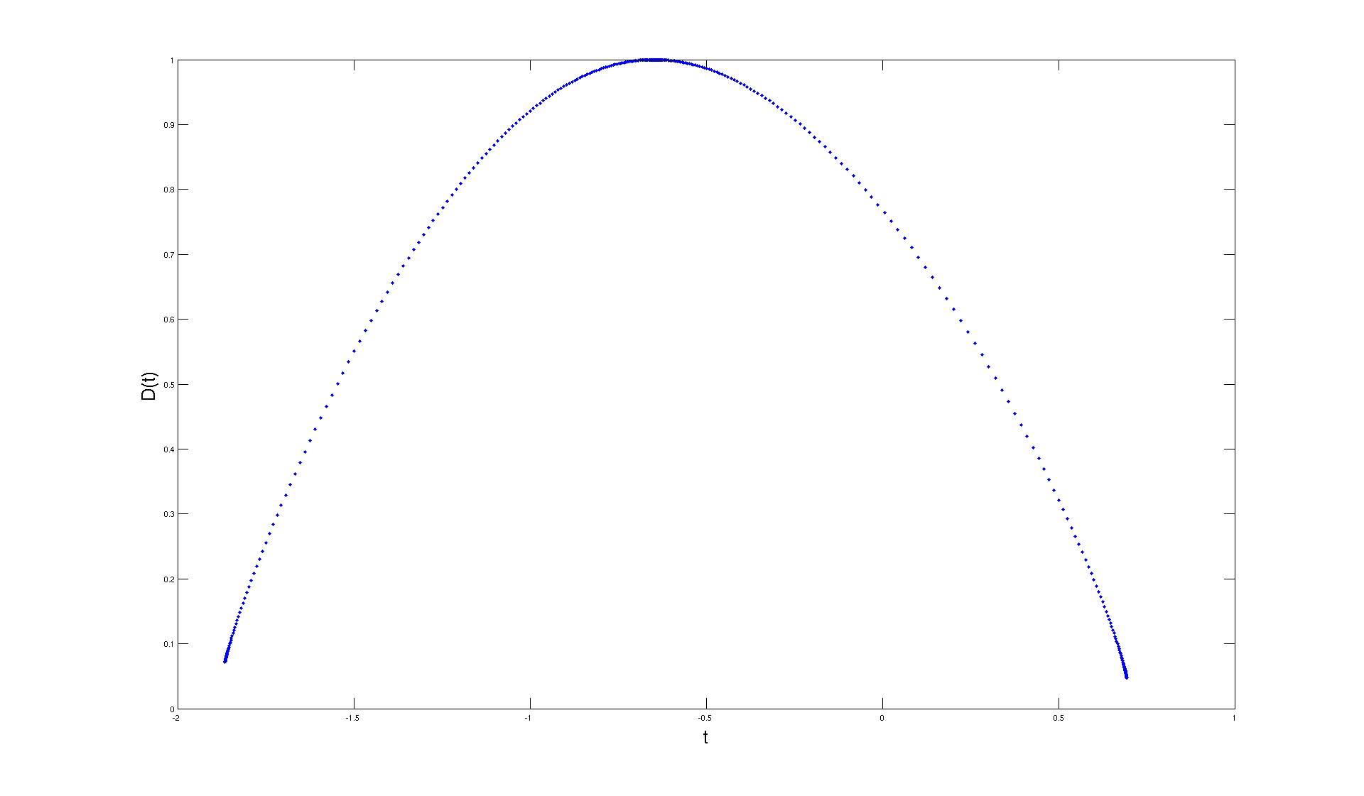
Figure 1. The function $D(t)$ for a baker map with $a=0.45$ and $g(u,v)=1.001+\cos(2\pi v)$.

4. Proofs

4.1. Proofs from section 2

Let $(\psi_{t,n})_{n\geqslant 0}$ and $M_{t}>0$ be as defined in Lemma 1, and denote $g_{t}:=e^{-t}g$.

Proof of Theorem 1.

1. Let $\theta\in\Theta$ such that $\Gamma_{t}\left(\theta\right)<0$. There are $\delta>0$ and integers $n_{1}<n_{2}<\dots$ such that

   $$\frac{d}{dx}f_{t}^{n_{j}}\left(T^{-n_{j}}\theta,x\right)_{|x=0}=\prod_{i=1}^{n_{j}}g_{t}\left(T^{-i}\theta\right)\leqslant e^{-\delta n_{j}}$$ (19)

   for all $j\in\mathbbm{N}$. As $\frac{d^{2}}{dx^{2}}f_{t}^{n_{j}}\left(T^{-n_{j}}\theta,x\right)<0$ for all $x\in(0,\infty)$ (cf. Remark 1), we have

   $$\varphi_{t}\left(\theta\right)\leqslant\psi_{t,n_{j}}\left(\theta\right)=f_{t}^{n_{j}}\left(T^{-n_{j}}\theta,M_{t}\right)\leqslant e^{-\delta n_{j}}M_{t}\mathop{\longrightarrow}\limits^{j\rightarrow\infty}0\,.$$

2. Let $\theta\in\Theta$ such that $\Gamma_{t}\left(\theta\right)>0$. There are $\delta>0$ and $C>0$ such that, for all $n\in\mathbbm{N}_{0}$,

   $$\prod_{i=1}^{n}g_{t}\left(T^{-i}\theta\right)\geqslant Ce^{\delta n}\,.$$ (20)

   For a contradiction, suppose $\varphi_{t}\left(\theta\right)=0$. Let $\varepsilon_{0}>0$ and $n_{0}\in\mathbbm{N}$ such that

   $$\inf_{x\in\left(0,\varepsilon_{0}\right)}\frac{h\left(x\right)}{x}\geqslant e^{-\delta}\hskip 10.00002pt\text{$\operatorname{and}$}\hskip 10.00002pt\psi_{t,n_{0}}\left(\theta\right)<\varepsilon_{0}\,.$$ (21)

   Let $k\left(n\right):=\max\left\{k\leqslant n:f_{t}^{k}\left(T^{-n}\theta,M_{t}\right)\geqslant\varepsilon_{0}\right\}$. As $k(n)<n$ if $n\geqslant n_{0}$, we have for $j\in\left\{0,\dots,n-k\left(n\right)-1\right\}$, i.e. for $n-j\in\left\{k\left(n\right)+1,\dots,n\right\}$,

   $$f_{t}^{n-k\left(n\right)-j}\left(T^{-n+k\left(n\right)}\theta,\varepsilon_{0}\right) \leqslant f_{t}^{n-k\left(n\right)-j}\left(T^{-n+k\left(n\right)}\theta,f_{t}^{k\left(n\right)}\left(T^{-n}\theta,M_{t}\right)\right)$$ (22)

   $$= f_{t}^{n-j}\left(T^{-n}\theta,M_{t}\right)\hskip 10.00002pt<\;\varepsilon_{0}\,.$$

   Using now (22) with $j=0$ and then (21) and (22) repeatedly, we obtain for $n\geqslant n_{0}$

   $$\psi_{t,n}\left(\theta\right) = f_{t}^{n}(T^{-n}\theta,M_{t})$$ (23)

   $$\geqslant f_{t}^{n-k\left(n\right)}\left(T^{-n+k\left(n\right)}\theta,\varepsilon_{0}\right)$$

   $$= g_{t}\left(T^{-1}\theta\right)h\left(f_{t}^{n-k\left(n\right)-1}\left(T^{-n+k\left(n\right)}\theta,\varepsilon_{0}\right)\right)$$

   $$\geqslant g_{t}\left(T^{-1}\theta\right)e^{-\delta}f_{t}^{n-k\left(n\right)-1}\left(T^{-n+k\left(n\right)}\theta,\varepsilon_{0}\right)$$

   $$= g_{t}\left(T^{-1}\theta\right)e^{-\delta}g_{t}\left(T^{-2}\theta\right)h\left(f_{t}^{n-k\left(n\right)-2}\left(T^{-n+k\left(n\right)}\theta,\varepsilon_{0}\right)\right)$$

   $$\geqslant g_{t}\left(T^{-1}\theta\right)e^{-\delta}g_{t}\left(T^{-2}\theta\right)e^{-\delta}f_{t}^{n-k\left(n\right)-2}\left(T^{-n+k\left(n\right)}\theta,\varepsilon_{0}\right)$$

   $$\vdots$$

   $$\geqslant \left(\prod_{i=1}^{n-k\left(n\right)}g_{t}\left(T^{-i}\theta\right)\right)(e^{-\delta})^{n-k\left(n\right)}\varepsilon_{0}\,.$$

   With (20) and the first estimate of (21) we obtain from (23)

   $$\psi_{t,n}\left(\theta\right)\geqslant Ce^{\delta\left(n-k\left(n\right)\right)}e^{-\delta(n-k(n))}\varepsilon_{0}=C\varepsilon_{0}\,,$$

   and therefore $\varphi_{t}(\theta)\geqslant C\varepsilon_{0}$. This contradicts the assumption.

3. This is a direct consequence of a) and b).

∎

Proof of Proposition 1..

Let $\theta\in\Theta\setminus N_{t}$, i.e. $\varphi_{t}(\theta)>0$. By definition of the functions $\psi_{t,n}$ we have

$$\psi_{t,n}(\theta)=g_{t}(T^{-1}\theta)\,h(\psi_{t,n-1}(T^{-1}\theta))$$

so that

$$\log\psi_{t,n}(\theta)=\log g_{t}(T^{-1}\theta)+H(\psi_{t,n-1}(T^{-1}\theta))+\log\psi_{t,n-1}(T^{-1}\theta)$$ (24)

where $H(x):=\log(x^{-1}h(x))$. As $h$ is concave and $h^{\prime}(0)=1$, $H$ extends to a decreasing function from $[0,\infty)$ to $(-\infty,0]$ with $H(0)=0$ and $H^{\prime}(0)=\frac{1}{2}h^{\prime\prime}(0)<0$. Iterating this identity $\ell$ times $(1\leqslant\ell\leqslant n)$ yields

$$\log\psi_{t,n}(\theta)=\sum_{k=1}^{\ell}\log g_{t}(T^{-k}\theta)+\sum_{k=1}^{\ell}H(\psi_{t,n-k}(T^{-k}\theta))+\log\psi_{t,n-\ell}(T^{-\ell}\theta)\,.$$ (25)

For fixed $\ell\in\mathbbm{N}$ we get in the limit $n\to\infty$

$$\log\varphi_{t}(\theta)=\sum_{k=1}^{\ell}\log g_{t}(T^{-k}\theta)+\sum_{k=1}^{\ell}H(\varphi_{t}(T^{-k}\theta))+\log\varphi_{t}(T^{-\ell}\theta)\,.$$ (26)

Recall that $\theta\in\Theta\setminus N_{t}$. Because of Theorem 1c), $\theta\in S_{t}$ if and only if $\sum_{k=1}^{\ell_{i}}\log g_{t}(T^{-k}\theta)=o(\ell_{i})$ along some subsequence $(\ell_{i})_{i\in\mathbbm{N}}$. In view of (26) this is equivalent to

$$\sum_{k=1}^{\ell_{i}}|H(\varphi_{t}(T^{-k}\theta))|+|\log\varphi_{t}(T^{-\ell_{i}}\theta)|=o(\ell_{i})\,.$$ (27)

As $H^{\prime}(0)<0$, there is a constant $C>0$ such that

$$C^{-1}\varphi_{t}(T^{-k}\theta)\leqslant|H(\varphi_{t}(T^{-k}\theta))|\leqslant C\varphi_{t}(T^{-k}\theta)\quad(k\geqslant 0)\,,$$ (28)

so that (27) is equivalent to

$$\sum_{k=1}^{\ell_{i}}\varphi_{t}(T^{-k}\theta)+|\log\varphi_{t}(T^{-\ell_{i}}\theta)|=o(\ell_{i})\,.$$ (29)

∎

4.2. Proof of Theorem 2

Remark 10.

We refer to [3, 6, 8] for the following well-known facts about topologically mixing Anosov diffeomorphisms:

1. The entropy function $h_{T}(\cdot):\mathcal{P}_{T}(\Theta)\to\mathbbm{R}_{\geqslant}$ is upper semi-continuous, as $T$ is expansive.

2. For Hölder-continuous functions $\phi,\psi:\Theta\rightarrow\mathbbm{R}$ the function $t\mapsto P(t\phi+\psi)$ is real analytic and strictly convex, unless $\phi$ is cohomologous to a constant, where $P(t\phi+\psi)$ denotes the topological pressure of $T$ for the potential $t\phi+\psi$.

We shall prepare three Lemmas, before we prove the theorem. In this section we assume that $\gamma_{\min}<\gamma_{\max}$. Recall that we defined $D(t)$ as

$$D(t)=\max\left\{\frac{h_{T}\left(\mu\right)}{\mu(-\log\|dT|E^{s}\|)}:\mu\in\mathcal{P}_{T}(\Theta)\mbox{ and }\gamma(\mu)=t\right\}.$$ (30)

Lemma 2.

$\dim_{H}(S_{t}^{\prime})=D(t)+1$ for $t\in(\gamma_{\min},\gamma_{\max})$. Furthermore, there is a real analytic function $q:(\gamma_{\min},\gamma_{\max})\rightarrow\mathbbm{R}$ such that for the unique equilibrium measure $\mu_{t}\in\mathcal{E}_{T}(\Theta)$ of the potential $q(t)\log g_{t}-D(t)\log\|dT|E^{s}\|$ the following holds:

$$\mu_{t}(S_{t})=1,\quad D(t)=\frac{h_{T}(\mu_{t})}{\mu_{t}(-\log\|dT|E^{s}\|)},\quad\text{and}\quad\dim_{H}(\mu_{t})=D(t)+1.$$ (31)

Proof.

For $\theta\in\Theta$ denote by $V^{s}_{loc}(\theta)$ the (suitably defined) local stable manifold of $T$ through $\theta$. Then [2, Theorem 12.2.2] asserts that $\dim_{H}(S_{t}^{\prime})=\dim_{H}(S_{t}^{\prime}\cap V^{s}_{loc}(\theta))+1$ for each $\theta\in S_{t}^{\prime}$. With the same argument as in [2, Example 7.2.5] one shows that $\dim_{H}(S_{t}^{\prime}\cap V^{s}_{loc}(\theta))$ coincides with the $u$-dimension of $S_{t}^{\prime}$ for the function $u=-\log\|dT|E^{s}\|$, and [2, Theorem 10.1.4] asserts that this $u$-dimension takes the value $D(t)$. (For the application of this last theorem observe that all Hölder potentials have a unique equilibrium state.) The assertions on $q(t)$ and $\mu_{t}$ follow from [2, Theorems 10.1.4 and 10.3.1] together with Corollary 3, [2, Lemma 10.1.6] and its proof. ∎

Lemma 3.

$D:(\gamma_{\min},\gamma_{\max})\rightarrow[0,1]$ is a real analytic function such that $D({\gamma_{c}^{-}})=1$, $D^{\prime\prime}({\gamma_{c}^{-}})<0$ and

$$D^{\prime}(t)=\left\{\begin{array}[]{ll}>0&\mbox{for }t\in(\gamma_{\min},{\gamma_{c}^{-}})\\ <0&\mbox{for }t\in({\gamma_{c}^{-}},\gamma_{\max})\end{array}\right..$$

Proof of Lemma 3.

For this proof, we will extend the proof of [2, Theorem 10.3.1]: Denote $(u,\Phi):=(-\log\|dT|E^{s}\|,\log g)$ and consider the real analytic function $Q\left(\delta,q,t\right):=P\left(q\left(\Phi-t\right)-\delta u\right)$. In that proof it is shown that the equations

$$\left\{\begin{array}[]{c}Q\left(D\left(t\right),q\left(t\right),t\right)=0\\ \frac{\partial Q}{\partial q}\left(D\left(t\right),q\left(t\right),t\right)=0\end{array}\right.$$ (32)

determine a real analytic function $\left(D,q\right):\left(\gamma_{\min},\gamma_{\max}\right)\rightarrow\mathbbm{R}^{2}$. These equations are further equivalent to

$$\left\{\begin{array}[]{l}h_{T}(\mu_{t})+\mu_{t}(q(t)\Phi-D(t)u)=q(t)t\\ \mu_{t}(\Phi)=t\end{array}\right..$$ (33)

Differentiating the first equality of (32) with respect to $t$ and using the second one, we obtain

$$D^{\prime}\left(t\right)=\frac{q\left(t\right)}{\frac{\partial Q}{\partial\delta}\left(D(t),q(t),t\right)}\,.$$ (34)

Similarly, differentiating the second equality of (32) and using (34), we obtain

$$q^{\prime}(t)=\frac{1}{\frac{\partial^{2}Q}{\partial q^{2}}\left(D(t),q(t),t\right)}\left(1-q(t)\frac{\frac{\partial^{2}Q}{\partial\delta\partial q}\left(D(t),q(t),t\right)}{\frac{\partial Q}{\partial\delta}\left(D(t),q(t),t\right)}\right).$$ (35)

From the second equality of (33) it follows $\mu_{t}\left(S_{t}^{\prime}\right)=1$ by Birkhoff’s theorem, whence $\mu_{t}\left(S_{t}\right)=1$ in view of Corollary 3. Moreover, from (33) we obtain

$$D(t)=\frac{h_{T}\left(\mu_{t}\right)}{\mu_{t}(u)}\,.$$ (36)

Furthermore, from $\left(\ref{eq:SRB}\right.$) we have

$$\left\{\begin{array}[]{l}Q\left(1,0,{\gamma_{c}^{-}}\right)=P\left(-u\right)=h_{T}\left(\mu_{\mathrm{SRB}}^{-}\right)-\mu_{\mathrm{SRB}}^{-}\left(u\right)=0\\ \frac{\partial Q}{\partial q}\left(1,0,{\gamma_{c}^{-}}\right)=\mu_{\mathrm{SRB}}^{-}\left(\varphi\right)-{\gamma_{c}^{-}}=0\end{array}\right.$$ (37)

so that

$$\left(1,0,{\gamma_{c}^{-}}\right)=\left(D({\gamma_{c}^{-}}),q({\gamma_{c}^{-}}),{\gamma_{c}^{-}}\right).$$ (38)

In view of (34), we have also

$$D^{\prime}\left({\gamma_{c}^{-}}\right)=0\,.$$ (39)

Finally, differentiating (34) we obtain

$$D^{\prime\prime}(t)=\frac{q^{\prime}(t)}{\frac{\partial Q}{\partial\delta}}-q(t)\,\frac{D^{\prime}(t)\frac{\partial^{2}Q}{\partial\delta^{2}}+q^{\prime}(t)\frac{\partial^{2}Q}{\partial\delta\partial q}+\frac{\partial^{2}Q}{\partial\delta\partial t}}{\left(\frac{\partial Q}{\partial\delta}\right)^{2}}$$ (40)

where all partial derivatives are evaluated at $(D(t),q(t),t)$. Observing that $\frac{\partial^{2}Q}{\partial\delta\partial t}=0$ and substituting (34) we obtain

$$D^{\prime\prime}(t)=\frac{1}{\frac{\partial Q}{\partial\delta}}\left(q^{\prime}(t)-D^{\prime}(t)\left(D^{\prime}(t)\,\frac{\partial^{2}Q}{\partial\delta^{2}}+q^{\prime}(t)\frac{\partial^{2}Q}{\partial\delta\partial q}\right)\right)$$ (41)

with all partial derivatives again evaluated at $(D(t),q(t),t)$. As we assume that $\gamma_{\min}<\gamma_{\max}$, the map $q\mapsto Q(\delta,q,t)$ is strictly convex (c.f. Remark 10). Hence, we obtain from (35) and (41) together with (38) and (39),

$$q^{\prime}\left({\gamma_{c}^{-}}\right)=\frac{1}{\frac{\partial^{2}Q}{\partial q^{2}}\left(1,0,\gamma_{c}^{-}\right)}>0\hskip 10.00002pt\text{$\operatorname{and}$}\hskip 10.00002ptD^{\prime\prime}\left({\gamma_{c}^{-}}\right)=\frac{q^{\prime}\left({\gamma_{c}^{-}}\right)}{\frac{\partial Q}{\partial\delta}\left(1,0,\gamma_{c}^{-}\right)}<0\,.$$ (42)

Now consider the curve $C:\left(\gamma_{\min},\gamma_{\max}\right)\rightarrow\left[0,1\right]\times\mathbbm{R}$ defined by $C(t)=\left(D(t),q(t)\right)$. In view of (38) and the first inequality of (42) this curve runs across the point $\left(1,0\right)$ in $t={\gamma_{c}^{-}}$ from left to right. As $\operatorname{sign}\left(D^{\prime}(t)\right)=-\operatorname{sign}\left(q(t)\right)$ by (34), $D^{\prime}(t)$ can change its sign only when $q(t)=0$, i.e. only if $t=\gamma_{c}^{-}$ and hence $D(t)=1$. Therefore $D^{\prime}(t)>0$ for $t<\gamma_{c}^{-}$ and $D^{\prime}(t)<0$ for $t>\gamma_{c}^{-}$. ∎

Recall that for $\nu\in\mathcal{P}(\Theta)$ the upper and lower point-wise dimensions at $\theta\in\Theta$ are defined by

$$\overline{d}_{\nu}(\theta):=\limsup_{r\rightarrow 0}\frac{\log\nu(B(\theta,r))}{\log r}\quad\mbox{and}\quad\underline{d}_{\nu}(\theta):=\liminf_{r\rightarrow 0}\frac{\log\nu(B(\theta,r))}{\log r}\,.$$ (43)

If $\overline{d}_{\nu}(\theta)=\underline{d}_{\nu}(\theta)$, we denote this with $d_{\nu}(\theta)$.

To formulate the next lemma we define the sets

$$N_{t}^{\geqslant}:=\left\{\theta\in\Theta:\Gamma\left(\theta\right)\geqslant t\right\}\quad\mbox{and}\quad N_{t}^{\leqslant}:=\left\{\theta\in\Theta:\limsup_{n\rightarrow\infty}\Gamma^{(n)}\left(\theta\right)\leqslant t\right\}.$$ (44)

Lemma 4.

Let $t\in(\gamma_{\min},\gamma_{\max})$. There is $\nu_{t}\in\mathcal{P}\left(\Theta\right)$ (which is in general not $T$-invariant) such that $\nu_{t}\left(S_{t}^{\prime}\right)=1$ with the following properties:

1. $d_{\nu_{t}}\left(\theta\right)=D\left(t\right)+1$ for $\nu_{t}$-a.e. $\theta\in\Theta$,

2. $\overline{d}_{\nu_{t}}\left(\theta\right)\leqslant D\left(t\right)+1$ for each $\theta\in S_{t}^{\prime}$,

3. $\underline{d}_{\nu_{t}}\left(\theta\right)\leqslant D\left(t\right)+1$ for each $\theta\in R_{t}^{\prime}$,

4. $\overline{d}_{\nu_{t}}\left(\theta\right)\leqslant D\left(t\right)+1$ for each $\theta\in N_{t}^{\leqslant}$ provided that $t<\gamma_{c}^{-}$, and

5. $\overline{d}_{\nu_{t}}\left(\theta\right)\leqslant D\left(t\right)+1$ for each $\theta\in N_{t}^{\geqslant}$ provided that $t>\gamma_{c}^{-}$.

Proof of Lemma 4.

We apply the very general result [2, Theorem 12.3.1] with slight modifications. Here is a dictionary between our notation and the notation from [2]:

$$\begin{array}[]{c|c}\text{Notation from \cite[cite]{[\@@bibref{}{Barreira}{}{}]}}&\text{Our notation}\\ \hline\cr\Lambda,\ f,\ \mathcal{M}&\Theta,\ T,\ \mathcal{P}_{T}(\Theta)\\ \kappa&1\\ \mathcal{P}^{+}(\,\cdot\,),\ \mathcal{P}^{-}(\,\cdot\,)&1,\ \gamma(\cdot)\\ \Phi^{+},\ \Phi^{-},\ \Psi^{+},\ \Psi^{-}&1,\ \log g,\ 1,\ 1\\ \alpha,\ \beta&1,\ t\\ K_{\alpha}^{+},\ K_{\beta}^{-}&\Theta,\ S_{t}^{\prime}\\ d^{+},\ d^{-}&1,\ D(t)\\ q^{+},\ q^{-}&1,\ q(t)\end{array}$$

We note that the assumption $\alpha\in\operatorname{int}\mathcal{P}^{+}(\mathcal{M})$ of [2, Theorem 12.3.1] is not satisfied in our setting, as $\mathcal{P}^{+}(\mathcal{M})=\{1\}=\{\alpha\}$. This assumption is only used to assure the existence of $q^{+}$ with the properties claimed in [2, Lemma 12.3.3]; but these properties are trivially satisfied in our case.

Now we can conclude immediately from [2, Theorem 12.3.1] and Lemma 2 that

$$\nu_{t}(S_{t}^{\prime})=\nu_{t}(K_{\alpha}^{+}\cap K_{\beta}^{-})=1\,,$$ (45)

and

$$d_{\nu_{t}}\left(\theta\right)=D\left(t\right)+1\quad\text{for $\nu_{t}$-a.e. $\theta\in\Theta$}\,,$$ (46)

$$\overline{d}_{\nu_{t}}\left(\theta\right)\leqslant D\left(t\right)+1\quad\text{for each $\theta\in S_{t}^{\prime}$}\,,$$ (47)

as

$$\dim_{H}(K_{\alpha}^{+})+\dim_{H}(K_{\beta}^{-})-\dim_{H}(\Lambda)=\dim_{H}(S_{t}^{\prime})=D\left(t\right)+1\,.$$ (48)

For the remaining proofs of assertions (3) to (5) we must modify some arguments from [2] slightly:

To (3) : We modify the proof of [2, Lemma 12.3.6] as follows. Since inequality (12.15) does no longer hold for all large $n$’s, but still for infinitely many $n$’s, several inequalities after the estimate (12.17) hold only for $r$’s such that $m\left(\theta,r\right)$ defined in (12.12) satisfies (12.15) in place of $n$. Choose a null sequence $(r_{k})_{k}$ of $r$’s in the above manner. Then we obtain the last two inequalities in the proof of Lemma 12.3.6 where both limits superior are replaced by the limits inferior.

To (4) : We modify the proof of [2, Lemma 12.3.6] again. Let $t\in\left(\gamma_{\min},{\gamma_{c}^{-}}\right)$ such that $q(t)<0$. Then, for $\delta>0$ and $\chi(\omega)\in N_{t}^{\leqslant}$, there is a $r(\omega)\in\mathbbm{N}$ such that for $n>r\left(\omega\right)$

$$q(t)\cdot\sum_{k=0}^{n}\left(\Phi^{s}\left(\left(\sigma^{-}\right)^{k}\omega^{-}\right)-t\right)>-\delta n|q(t)|.$$ (49)

Since we can obtain (12.17) from this estimate instead of (12.15), the proof is finished.

To (5) : Let $t\in\left({\gamma_{c}^{-}},\gamma_{\max}\right)$ such that $q(t)>0$. As in the proof of (4), for $\delta>0$ and $\chi\left(\omega\right)\in N_{t}^{\geqslant}$ there is a $r\left(\omega\right)\in\mathbbm{N}$ such that (49) holds for $n>r(\omega)$, and again we can obtain (12.17) from this estimate instead of (12.15). ∎

Lemma 5.

For $t\in\left(\gamma_{\min},\gamma_{\max}\right)$ we have $\dim_{H}\left(S_{t}^{\prime}\right)=\dim_{H}\left(R_{t}^{\prime}\right)=\dim_{P}\left(S_{t}^{\prime}\right)=D\left(t\right)+1$. Furthermore, $\dim_{H}(N_{t}^{\leqslant})=D(t)+1$ for $t\in\left(\gamma_{\min},\gamma_{c}^{-}\right]$ and $\dim_{P}\left(N_{t}^{\geqslant}\right)=D\left(t\right)+1$ for $t\in\left[{\gamma_{c}^{-}},\gamma_{\max}\right)$.

Proof of Lemma 5.

This follows from Lemma 4 with [2, Theorem 2.1.5] and [4, Proposition 2.3]. ∎

Remark 11.

Roughly speaking, each of the sets $S_{t}^{\prime}$ and $R_{t}^{\prime}$ is locally the product of a $D(t)$-dimensional subset of the local stable manifold and the complete local unstable manifold.

Proof of the Theorem 2.

As $S_{t}^{\prime}\subseteq S_{t}\subseteq R_{t}^{\prime}$, we obtain $\dim_{H}\left(S_{t}\right)=D\left(t\right)+1$ for $t\in\left(\gamma_{\min},\gamma_{\max}\right)$ from Lemma 5. For the remaining arguments observe also the monotonicity properties of $t\mapsto D(t)$ from Lemma 3.

Let $t\in\left(\gamma_{\min},{\gamma_{c}^{-}}\right]$. Firstly, $D(t)+1=\lim_{t^{\prime}\nearrow t}D(t^{\prime})+1=\lim_{t^{\prime}\nearrow t}\dim_{H}(S_{t^{\prime}})\leqslant\dim_{H}(N_{t})$, as $S_{t^{\prime}}\subseteq N_{t}$. Secondly, from Theorem 1 we have $N_{t}\subseteq\left\{\Gamma\leqslant t\right\}\subseteq R^{\prime}_{t}\cup N^{\leqslant}_{t}$. Thus, $\dim_{H}(N_{t})\leqslant\max\{\dim_{H}(R^{\prime}_{t}),\dim_{H}(N^{\leqslant}_{t})\}=D(t)+1$, and it follows that $\dim_{H}(N_{t})=D(t)+1$.

Now, let $t\in\left[{\gamma_{c}^{-}},\gamma_{\max}\right)$. Firstly, $D(t)+1=\lim_{t^{\prime\prime}\searrow t}D(t)+1=\lim_{t^{\prime\prime}\searrow t}\dim_{H}(S_{t^{\prime\prime}})\leqslant\dim_{H}(\Theta\setminus N_{t})$, as $S_{t^{\prime\prime}}\subseteq\Theta\setminus N_{t}$. Secondly, from Theorem 1 we have $\Theta\setminus N_{t}\subseteq N^{\geqslant}_{t}$. Thus, $\dim_{H}(\Theta\setminus N_{t})\leqslant\dim_{P}(\Theta\setminus N_{t})\leqslant\dim_{P}(N_{t}^{\geqslant})=D(t)+1$, and it follows that $\dim_{H}(\Theta\setminus N_{t})=\dim_{P}(\Theta\setminus N_{t})=D(t)+1$. ∎

4.3. Proof of Theorem 3

Proof.

To (2): Let $t\in[\gamma_{c}^{-},\gamma_{\max})$. For $t^{\prime}\in(t,\gamma_{\max})$ and $\nu_{t^{\prime}}\in\mathcal{P}(\Theta)$ from Lemma 4 it follows $\nu_{t^{\prime}}\left(\bigcup_{k\in\mathbbm{N}}\{\varphi_{t}>1/k\}\right)=\nu_{t^{\prime}}(\Theta\setminus N_{t})\geqslant\nu_{t^{\prime}}(S_{t^{\prime}})=1$, whence there is a $k\in\mathbbm{N}$ s.t. $\nu_{t^{\prime}}(\{\varphi_{t}>1/k\})>0$. Denoting the restriction of $\nu_{t^{\prime}}$ to this set by $\tilde{\nu}_{t^{\prime}}$ we obtain $\dim_{H}(\{\varphi_{t}>1/k\})\geqslant\dim_{H}(\tilde{\nu}_{t^{\prime}})\geqslant D(t^{\prime})+1$ by [2, Theorem 2.1.5], as $d_{\tilde{\nu}_{t^{\prime}}}=d_{\nu_{t^{\prime}}}=D(t^{\prime})+1$ holds $\tilde{\nu}_{t^{\prime}}$-a.e.. Therefore, $\dim_{H}(\{\varphi_{t}>1/k\})\geqslant\lim_{t^{\prime}\searrow t}D(t^{\prime})+1=D(t)+1$, and it follows from the first product rule of [11, Theorem 3] that

$$\dim_{H}(\mathcal{A}_{t})\geqslant\dim_{H}\left(\{\varphi_{t}>1/k\}\times[0,1/k]\right)\geqslant\dim_{H}(\{\varphi_{t}>1/k\})+\dim_{H}([0,1/k])\geqslant D(t)+2.$$

On the other hand, Theorem 2 in conjunction with the last product rule of [11, Theorem 3] implies

$$\dim_{P}(\mathcal{A}_{t})\leqslant\dim_{P}\left(\Theta\setminus N_{t}\times[0,M_{t}]\right)\leqslant\dim_{P}(\Theta\setminus N_{t})+\dim_{P}([0,M_{t}])=D(t)+2,$$

so that $\dim_{P}(\mathcal{A}_{t})=\dim_{H}(\mathcal{A}_{t})=D(t)+2$.

To (1): Let $t\in(\gamma_{\min},\gamma_{c}^{-}]$. From (2) and Theorem 2 it follows $\dim_{P}(\mathcal{A}_{t})\geqslant\dim_{H}(\mathcal{A}_{t})\geqslant\dim_{H}(\mathcal{A}_{\gamma_{c}^{-}})=D(\gamma_{c}^{-})+1=3$, which finishes the proof. ∎

References

- [1] L. Arnold. Random Dynamical Systems. Springer, 2 edition, 2003.
- [2] L. Barreira. Dimension and recurrence in hyperbolic dynamics. Birkhäuser, 2008.
- [3] R. Bowen. Equilibrium states and the ergodic theory of Anosov diffeomorphisms. Springer, 2 edition, 2007.
- [4] K. Falconer. Techniques in Fractal Geometry. Wiley, 1997.
- [5] G. Keller. A note on strange nonchaotic attractors. Fund. Math, 151:139–148, 1996.
- [6] G. Keller. Equilibrium States in Ergodic Theory. Cambridge University Press, 1998.
- [7] G. Keller, H. Jaffri, and R. Ramaswamy. Generalized synchronozation in chaotically driven systems. In preparation, 2012.
- [8] W. Parry and M. Pollicott. Zeta functions and the periodic orbit structure of hyperbolic dynamics. Soc. Math. de France, 1990.
- [9] J. Schmeling. Entropy preservation under markov coding. Journal of Statistical Physics, 104:799–815, 2001.
- [10] R. Sturman and J. Stark. Semi-uniform ergodic theorems and applications to forced systems. Nonlinearity, 13:113, 2000.
- [11] C. Tricot. Two definitions of fractional dimension. Math. Proc. Camb. Phil. Soc., 91:57–74, 1982.