Mapping Strategies for the PERCS Architecture

Abstract

The PERCS system was designed by IBM in response to a DARPA challenge that called for a high-productivity high-performance computing system. The IBM PERCS architecture is a two level direct network having low diameter and high bisection bandwidth. Mapping and routing strategies play an important role in the performance of applications on such a topology. In this paper, we study mapping strategies for PERCS architecture, that examine how to map tasks of a given job on to the physical processing nodes. We develop and present fundamental principles for designing good mapping strategies that minimize congestion. This is achieved via a theoretical study of some common communication patterns under both direct and indirect routing mechanisms supported by the architecture.

1 Introduction

The PERCS supercomputer is the latest in a line of high performance computing systems from IBM [14]. Previously known as “POWER7-IH” [14] and commercialized as the Power 775 [11], this system can incorporate up to 64K Power7 processors with a high-radix, high-bisection-bandwidth interconnect based on the IBM Hub Chip [3, 2]. The system is a direct outcome of the similarly named PERCS project (Productive Easy-to-use Reliable Computing System) that was initiated by DARPA in 2002 with the goals of providing state-of-the-art sequential performance as well as interconnect performance exceeding the state-of-the-art by orders of magnitude. With its integrated interconnect and storage, the PERCS system is expected to provide high sustained performance on a broad class of HPC workloads.

An important aspect of the PERCS architecture is the two-level direct-connect topology provided by a Hub chip [2]. In this setup, Hub chips (or nodes) are grouped in the form of cliques (called supernodes) and these cliques are then inter-connected. A total of 47 links out of each Hub chip create an interconnect with no more than three hops required to reach any other Hub. Furthermore, the denseness of this interconnect yields high bisection bandwidths and makes the system suitable for communication intensive workloads. The PERCS topology is noteworthy in that the multiple links can be setup between a pair of supernodes.

A fundamental issue in parallel systems is the mapping of tasks of a given job to the processors based on the communication pattern of the job and the characteristics of the underlying topology. The mapping determines the congestion on the network links and hence the performance of the application. The mapping problem has been extensively studied with respect to various communication topologies such as the torus, hypercube and fat-tree interconnects (see, for example, [1, 6, 8, 9]). Prudent mapping not only results in improved communication bandwidth but also less inter-job interference.

To the best of our knowledge, the work of Bhatale et al[5] is the only prior study of the mapping problem on the PERCS architecture. They consider a sample set of communication patterns ( 2D 5-point stencil, 4D 9-point stencil, Multicast) and developed heuristics to perform the mapping. The idea was to divide the given job into blocks and partition the processors into blocks (where each block consists of neighboring processors); the job blocks are then mapped onto the processor blocks in a random manner. Different heuristics were obtained by changing the block size. They conducted an extensive experimental evaluation to compare these heuristics.

Our contributions. The main contribution of this paper is to initiate a systematic approach for designing good mapping strategies for the PERCS architecture. Our aim is to develop mapping strategies based on sound theoretical underpinnings derived via a formal analysis of the system.

A complete study of the mapping problem for the PERCS architecture would ideally cater to handling multiple jobs executing simultaneously on the system; the jobs having potentially different predominant communication patterns. However, this can be a challenging task given the fact that the architecture is very recent and there is lack of principled prior study on this architecture. Being an initial study, we restrict the scope of this paper as follows: (i) we consider only a single system-wide job; (ii) we only consider the load on the links (link congestion), ignoring other protocol overheads – this aids in focusing on the critical architectural aspects; and (iii) we consider only two (but very contrasting) communication patterns. We note that Bhatale et al.[5] also consider only a single system-wide job and only a selected set of communication patterns. We believe that the concepts and theoretical principles developed here will guide in a complete study of this problem.

Though our study has the above-mentioned limitations, we consider a wide range of system configurations determined by the following parameters:

• The system size (number of supernodes)

• The number of links connecting any pair of supernodes

• Two different routing schemes: (i) direct routing, where data is sent over the direct link(s) connecting the supernodes; (ii) indirect routing, where an intermediate supernode is used as a bounce point for redirecting data in order to improve the load balance.

In comparison, we note that Bhatale et al.[5] consider only two system sizes (64 supernodes and 304 supernodes) whereas we consider a wider range system sizes.

An important aspect of the PERCS architecture is that the number of links between pairs of supernodes can be varied. This wealth of choice in system connectivity needs to be carefully considered based on the needs of the workloads that will be executed on the system. For randomized workloads like those exemplified by the Graph500 [10] and RandomAccess [7] benchmarks, high connectivity will be beneficial. For many HPC workloads, a lower level of connectivity may suffice. For instance, large classes of HPC workloads have been shown to have fairly low-radix inter-task partnering patterns [4]. For such workloads, choosing a topology with a lower number of links between supernode pairs may result in considerable cost savings. An important feature of our study is that the number of links between a pair of supernodes is taken as a parameter and can be varied. In comparison, prior work allow only a single link between a pair of supernodes.

The two communication patterns that we study are:

• Halo (two-dimensional 5-point Stencil) [13]: Tasks are arranged in the form of a 2-D grid and each task communicates with its north, east, south and west neighbors.

• Transpose [7]: Tasks are arranged in the form of a 2-D grid and each task communicates with all the tasks in the same row and column as that of the given task.

Note that these sample patterns are contrasting in nature. While the communication pattern of Halo is sparse, that of transpose is a fairly dense. Halo is indicative of the small-partner-count patterns that dominate HPC workloads. Transpose is indicative of the performance of workloads that use spectral methods such as the FFT. We next highlight some of the important contributions of our study with respect to each of these patterns.

For the Halo pattern, Bhatale et al.[5] devised a mapping heuristic based on random mapping of task blocks to processor blocks (as mentioned earlier). We devise a deterministic strategy to map the task blocks to the processor blocks based on the theoretical properties of modulo-arithmetic, that removes the randomness and provides up to a factor 2 improvement in throughput under direct routing.

To the best of our knowledge, our work is the first to study the transpose pattern for the PERCS architecture. We argue that direct routing offers better throughput than indirect routing for this pattern. This is in strong contrast to all the patterns considered by Bhatale et al.[5] for which they experimentally demonstrated that the indirect routing is superior. This shows that there are communication patterns that benefit under direct routing and therefore a study of the mapping problem would be incomplete without considering direct routing.

We also present experimental evaluation of the various mapping schemes using a simulator for computing throughput. Our experiments confirm that the mapping based on mod-arithmetic is superior to the random mapping schemes for the Halo pattern under direct routing by a factor of up to two. The experiments also validate that direct routing is better than indirect routing for transpose while indirect routing is better than direct routing for Halo.

Apart from PERCS, the concepts developed in this paper are more broadly applicable to a larger class of topologies categorized as multi-level direct networks with all-to-all connections at each level. The Dragonfly topology [12] that was introduced in 2008 articulates the technological reasons for using high-radix routers while lowering the number of global cables that criss-cross the system.

2 PERCS Architecture

Our goal in this paper is to find a “good” mapping of tasks to compute elements for a variety of communication patterns and routing schemes. We lay the groundwork in this section by describing the PERCS interconnection topology. While discussing the topology and routing scheme, we simplify certain details of the actual system in order to make the model more understandable.

The basic unit of the PERCS network is a Quad Chip Module or node which consists of four Power7 processors [15]. By virtue of being located in a tight package, the four Power7 chips are fully connected to each other by very high bandwidth links operating at 48 GB/s/direction. In general, intra-QCM communication is high enough to be considered “free” for the purposes of this study. Eight nodes are physically co-located in a drawer. The nodes in a drawer are connected in the form of a clique using bidirectional copper LL-links (i.e., each pair of nodes in a drawer is connected by a dedicated LL-link) that provide $21{\rm~{}GB/s/direction}$ of bandwidth. For ease of exposition, we will assume that each node also has a self-loop LL-link resulting in a node having eight LL-links connecting it to itself and the other nodes within the drawer.

Four drawers combine to form a supernode with each pair of nodes in different drawers connected using a dedicated bidirectional optical LR-link operating at $5{\rm~{}GB/s/direction}$. Every node has twenty-four LR links that connect it to each of the twenty-four nodes in the other three drawers.

A supernode thus consists of a clique of thirty-two nodes connected by two type of links: intra-drawer LL-links operating at $21{\rm~{}GB/s/direction}$ and inter-drawer LR-links operating at $5{\rm~{}GB/s/direction}$. In the rest of the paper, we drop the designation “/direction” noting that all bandwidths are treated as the bandwidth per direction. Figure 1(a) highlights one exemplar LL and LR link in a supernode. We shall use the term L to denote both LL and LR-links. Multiple supernodes are in turn connected via bidirectional D-links. Each D link operates at $10{\rm~{}GB/s}$ with the system design permitting multiple D-links between pairs of supernodes.

We shall use the term ${n_{s}}$ to denote the number of supernodes in the system and the term ${n_{d}}$ to denote the number of D-links between pairs of supernode. The tuple (${n_{s}}$, ${n_{d}}$) specifies a system. For instance, a $(32,4)$ system consists of $32$ supernodes with each pair of supernodes being connected via four D-links. The implementation requires that ${n_{d}}$ must divide $32$, the number of nodes in a supernode yielding systems with six different ${n_{d}}$ values: $\{1,2,4,8,16,32\}$.

The value of $n_{d}$ determines the D-link wiring across supernodes. Nodes within each supernode are divided into ${n_{d}}$ buckets, with each bucket having $32/{n_{d}}$ nodes. A D-link connects each bucket to the corresponding bucket in every other supernode – therefore each bucket must have ${n_{s}}$ D-links originating from it connecting it to every supernode in the system (similar to our treatment of the LL links, we assume a self-loop D link for ease of exposition). Since a bucket may have fewer nodes than are in a supernode, a node may be attached to multiple D links. We call this the ${n_{d}}D$-topology and next describe a template that specifies where these $n_{s}$ D-links connect. Let $W$ be the number of nodes in a bucket. Then, the $j^{\rm th}$ bucket (where $0\leq j<n_{d}$) consists of nodes numbered $\{jW,1+jW,\ldots,(W-1)+jW\}$. Each bucket has $n_{s}$ D-links connecting it to every supernode in the system. Within this bucket, the D-link connecting to supernode $b$ will originate from the node $v$ numbered $jW+(b\bmod W)$. We refer to this as the supernode $b$ being incident on the node $v$. Thus, each supernode will be incident on $n_{d}$ nodes.

Illustration: Figure 1(b) illustrates the D-link connectivity for a 32-supernode system with two D-links between every pair of supernodes. This is an ($n_{s}=32$, $n_{d}=2$) system that uses a $2D$-topology. In this system, supernode $1$ is incident on nodes $\{1,17\}$. Since $n_{d}=2$, there are two buckets each with sixteen nodes. Bucket 0 consists of nodes in the first two drawers numbered $\{0,1,\ldots,15\}$. Bucket 1 consists of the remaining two drawers with nodes numbered $\{16,17,\ldots,31\}$. Thirty-two D links go from each bucket to the thirty-two supernodes in the system. Every supernode uses this template. Thus supernodes 0 and 16 are incident on node 0 in each bucket while supernodes 2 and 18 are incident on node 2 in each bucket. The figure explicitly calls out the D-link connectivity between supernode 2 on the left and supernode 11 on the right. Two D-links connect this pair of supernodes. In bucket 0, the D-link is between node 11 of supernode 2 and node 2 of supernode 11. The same template is followed in bucket 1, with a D-link between node 27 of supernode 2 (which is the same as node 11 in bucket 1) and node 18 of supernode 11 (which is the same as node 2 in bucket 1).

As a second example, consider a ($n_{s}=16$, $n_{d}=8$) system. This system will have eight buckets per supernode each with four nodes. Bucket 0 will contain the four nodes in the first half of the first drawer: $\{0,1,2,3\}$ while bucket 7 will consist of the nodes in the second half of the last drawer: $\{28,29,30,31\}$

Any node is indexed by a tuple $\langle a,u\rangle$, where $a$ is the supernode number ($0\leq a\leq n_{s}-1$) and $u$ is the node number ($0\leq u\leq 31$). For instance, $\langle 11,13\rangle$ will be node $13$ in supernode $11$.

We next define the notion of D-port utility factor, which is useful in our analysis. The D-port utility factor $h$ is defined to be the average number of D-links originating from each node; formally, we define $h=n_{s}/W$. Equivalently $h=n_{s}n_{d}/32$. For expositional ease, we only consider systems where $h$ is an integer in this paper. For instance, the $32$-supernode system of Figure 1(b) has $h=2$ (i.e., two D-links originate and terminate at every node). This terminology arises from the fact that nodes are equipped with optical transceiver ports that accept the D-links and $h$ counts the number of D-ports used per node.

The Power 775 implements a maximum of $16$ D-ports at every node implying an $h$ factor of at most $16$. This means that $n_{s}n_{d}$ must be at most 512 capping the maximum system size at 512 supernodes.

(a) Supernode		(b) D-link connectivity

Figure 1: Illustration of supernode and D-link connectivity

The design supports two routing methods for inter-supernode communication. In the direct routing scheme, the D-links directly connecting these supernodes are used to transfer data. In the indirect routing scheme, an intermediate supernode is used for redirecting data to the destination supernode. The direct routing scheme employs one D traversal, while the indirect routing scheme uses two D traversal. The advantage with indirect routing is in its ability to offer better load balancing [3, 14]. A formal description of these routing schemes will be provided in subsequent sections.

3 Problem Statement

We now define the mapping problem precisely and introduce different communication patterns studied in the paper.

Every supernode has 32 nodes, each containing four Power7 processors. We assume that each processor can execute a compute task yielding $128\times{n_{s}}$ tasks system-wide. The communication employed by the tasks in a job constitutes a communication pattern that can be visualized as a graph where the vertices denote tasks and directed edges denote inter-task communication. The problem we investigate here is to map tasks to processors so as to maximize system throughput taking both topology and routing into consideration.

Prior work has observed that a small number of low-radix partnering patterns dominate most HPC workloads [4]. Our analysis focuses on the following two patterns: Halo and Transpose; it shows how task mapping can be improved for high-radix interconnects such as that found in PERCS.

Throughput Analysis: For our analysis, we assume that each task has a total of one unit of data to send to all of its neighbors. In the case of Halo, the amount of data sent to the neighbors is uniform. In the case of transpose, $(1/2)$ unit of is distributed uniformly among the tasks in the same row and $(1/2)$ unit is distributed uniformly among the tasks in the same column. In the case of Halo, each task $x$ will send $(1/4)$ units of data to each of its four neighbors; in the case of transpose job consisting of $32$ rows and $64$ columns, each task $x$ will send $(1/128)$ unit of data to each task on the same row and $(1/64)$ unit of data to each task on the same column.

Consider a job $J$ and a function $\pi$ mapping the tasks of $J$ to the physical Power7 processors. Data transfer between task $x$ and $y$ takes place between the physical processors $u=\pi(x)$ and $v=\pi(y)$. The specific routing choice (direct or indirect) employed determines the set of paths over which the data is sent and thence the amount of load placed on every link in the paths. We then obtain the total load $\ell(e)$ on a link $e$ by calculating the load contributions from every pair of communicating tasks that use that link.

Let $L_{LL}$ be the maximum of $\ell(e)$ over all the LL-links. Similarly, let $L_{LR}$ and $L_{D}$ denote the maximum total load over all the LR and D-links. Recall that the LL, LR and D links have different bandwidths of 21, 5, and 10  GB/s respectively. These bandwidth differences arise from the very different cost, power, and capabilities that each transport offers. Continuing our analysis, we normalize these numbers by dividing $L_{LL}$ by 21, $L_{LR}$ by $5$ and $L_{D}$ by 10. Let $t=\max\{L_{LL}/21,L_{LR}/5,L_{D}/10\}$. The value $t$ is a measure of congestion in the system and a measure of the overall time it will take for the job to complete execution. The value $1/t$ provides the throughput per task. In other words, $(1/t)$ is maximum amount of data that every task can send so that every LL, LR and D-link gets a total load of at most 21  GB/s, 5  GB/s and 10  GB/s respectively. If each task sends $(1/t)$ GB of data, then the whole communication will be completed in one second. Since four tasks execute on each node, the value $(4/t)$ provides the throughput per node.

We define the throughput of the mapping $\pi$ to be $\tau(\pi)=(4/t){\rm~{}GB/s}$. We also define throughput with respect each type of link: (i) $\tau_{{\rm LL}}(\pi)=(1/L_{LL})\times 4\times 21$; (ii) $\tau_{{\rm LR}}(\pi)=(1/L_{LR})\times 4\times 5$; (iii) $\tau_{{\rm D}}(\pi)=(1/L_{D})\times 4\times 10$. Notice that $\tau(\pi)$ is the minimum over the above three quantities.

Mapping Problem: Given a specific job consisting of $n=128n_{s}$ tasks and a specific routing scheme, the problem is to devise a mapping $\pi$ having high throughput $\tau(\pi)$.

4 Direct Routing

We first describe the direct routing scheme. Then, we study the mapping problem for the Halo and Transpose patterns.

4.1 Routing Scheme

We first describe intra-supernode routing, which is used for communication between two nodes within the same supernode. Two types of routing schemes are supported for this scenario.

• Single Hop: All the communication between any two nodes is performed via the LL or LR link connecting them. Figure 1(a) shows the single-hop route for communication between nodes 1 and 4, as well as nodes 1 and 18.

• Striped: Communication between nodes $u$ and $v$ is directed through one of the nodes in the same drawer as $u$ giving rise to LL-LL or LL-LR path. A message from $u$ to $v$ is striped into multiple packets that are sent over the above eight paths. If node $u$ has 1 unit of data to send, each path will receive $(1/8)$ units of data.

To illustrate striped routing, first consider the case of intra-drawer communication with node 0 sending data to node 1. This transfer will be striped over eight paths of the form $0\rightarrow x\rightarrow 1$, where any of the eight nodes ($\{0,1,\ldots,7\}$) present in the drawer can be used as the bounce point. Note that we permit nodes 0 and 1 to also act as the bounce point; in this case, we imagine that the LL self-loop at the node is utilized. Next consider the case of inter-drawer communication with node 0 sending data to node 8. These nodes are in different drawers and we stripe it over eight paths of the form $0\rightarrow x\rightarrow 8$, where the bounce point $x$ can be any of the eight nodes present in the first drawer ($\{0,1,\ldots,7\}$). If the amount of data is 1 unit, $1/8$ units of the sent will be sent over each path. As before, node 0 can itself also act as a bounce point. We thus stripe intra-drawer communication over eight paths of the form LL-LL and inter-drawer communication over eight paths of the form LL-LR.

Striped routing adds more load on the LL links compared to single-hop routing. However, it enables better link load balancing by using more of the higher bandwidth LL links. In the rest of the paper, we only consider striped routing for intra-supernode communications.

We next describe inter-supernode communication under direct routing when nodes $u$ and $v$ need to communicate but are located in different supernodes. The destination supernode in incident on the source supernode through ${n_{d}}$ D-links. Data transfer between the nodes is striped over these ${n_{d}}$ links through paths of the form L $\rightarrow$ D $\rightarrow$ L. If node $u$ has 1 unit of data to send, each path will receive $1/n_{d}$ units of data.

For an illustration, refer to Figure 1 (b) and consider node $1$ in supernode $2$ needing to send data to node $31$ in supernode $11$. This communication will be striped over the two D-links shown in the figure utilizing the following L-D-L paths: (i) $\langle 2,1\rangle\rightarrow\langle 2,11\rangle\rightarrow\langle 11,2\rangle\rightarrow\langle 11,31\rangle$; (ii) $\langle 2,1\rangle\rightarrow\langle 2,27\rangle\rightarrow\langle 11,18\rangle\rightarrow\langle 11,31\rangle$.

4.2 Principles

In this section, we discuss some general principles that are useful in designing good mapping strategies for a general communication pattern $J$.

Developing a mapping strategy proceeds in two steps. In the first step, we map each task to a supernode; in the second step, we map the tasks to individual nodes within the supernodes. Note that the D-links are used only for inter-supernode communication causing the D-link throughput to be determined solely by the first mapping. D links are the long global cables in the system.

Our experience suggests that it is often difficult to optimize on all the three types of throughputs. A useful rule of thumb is to focus on D-link throughput while designing the first mapping and consider LR-link and LL-link throughputs in the second step. Decomposing the mapping problem in this manner makes it tractable.

Let us now consider the first step of mapping tasks to supernodes. We view the mapping as a process of coloring of the vertices (i.e., tasks) in the communication graph using the set of colors $\{0,1,2,\ldots,n_{s}-1\}$. We must ensure that all the colors appear an equal number of times ($128$ times, since each supernode has 128 processors). In order to obtain high D-link throughput, the coloring should ensure two properties:

• Load Reduction: A color class must form a dense subgraph with as few outgoing edges as possible. Doing so minimizes the total load contribution on the D-links.

• Load Distribution: For any pair of color classes, the number of edges between the color classes must be minimized. This way the load on the bundle of $n_{d}$ D-links connecting any pair of supernodes will be minimized. One way to achieve the above goal is to ensure that for each color class, the neighbors of the tasks in the color class are uniformly distributed across other color classes.

Let us now consider the second step of mapping tasks to individual nodes. Consider an $L$-link going from a node $u$ to a node $v$. For inter-supernode communication, link $e$ is used both when $u$ sends data to any supernode incident on $v$ and when $v$ receives data from any supernode incident on $u$. So, we must ensure that the eight tasks mapped to nodes $u$ and $v$ do not have their neighbors concentrated on the above two types of supernodes. Doing so reduces the load imposed on $e$ due to inter-supernode communication.

4.3 Mapping Strategies for Halo

In this section, we consider the Halo pattern. We first discuss certain natural strategies and then present a scheme whose design is based on the properties of modulo arithmetic. We shall mainly focus on the D-link throughput. However, we will ensure that LR-link and LL-link throughput are not significantly compromised in the process.

Let number of processors $n$ is given by $n=128n_{s}$, since there are $128$ processors in a supernodes; the number of tasks in the job is also $n$. Consider the job as a $P\times Q$ grid consisting of $P$ rows and $Q$ columns such that $PQ=n=128n_{s}$. Without loss of generality, assume that $P\leq Q$. A simple strategy for mapping any pattern is to map the tasks sequentially to the processors. This can be considered as a default mapping: the $128n_{s}$ processors are indexed sequentially and the task having rank $j$ is mapped to the processor having index $j$. Bhatale et al. have proposed certain natural strategies that are better than default mapping based on the idea of creating blocks [5]. We present an overview of these strategies.

Blocking Strategies

Let $\alpha$ and $\beta$ be numbers such that they divide $P$ and $Q$, respectively. The $P\times Q$ grid is divided into blocks of size $\alpha\times\beta$ resulting in $(P/\alpha)\times(Q/\beta)$ blocks. Bhatale et. al. [5] obtain different mapping schemes by choosing different values for $\alpha$ and $\beta$:

• Node blocking: $\alpha\times\beta$ = $2\times 2$; fits in a node.

• Drawer blocking: $\alpha\times\beta$ = $4\times 8$; fits in a drawer.

• Supernode blocking: $\alpha\times\beta$ = $8\times 16$; fits in a supernode.

The next step is to map the tasks to processors which we accomplish by dividing processors also into blocks: in the case of drawer blocking, each drawer constitutes a processor block; in the case of node and supernode blocking, each node and each supernode become a block, resp. Processor and task blocks are indexed in a canonical manner. Then the task blocks are mapped to processor blocks in one of the two ways:

• Sequential: A task block having index $j$ is mapped to processor block having index $j$.

• Random: Task blocks are mapped to processor blocks in a random manner.

Bhatale et al.[5] proposed the above schemes and presented an experimental evaluation based on the BigSim simulator [16]. Below, we present an theoretical analysis of the throughput of these schemes. Based on the ideas discussed here we develop an improved mapping strategy.

Blocking Strategies (An Informal Analysis)

In the Halo pattern, a block is a dense subgraph and so, creating blocks reduces load on the different types of links. We analyze the D-link throughput of the blocking schemes. Consider an $\alpha\times\beta$ block. With respect to the task grid, the number of edges going out of the four sides this block is $2(\alpha+\beta)$. Each of these edges carry $(1/4)$ units of data (since each task sends $(1/4)$ units of data to each of its four neighbors). Thus, the amount of data going out of each block is $(\alpha+\beta)/2$. Each supernode has $128/(\alpha\beta)$ blocks. If no two adjacent task blocks are mapped to the same supernode, the data leaving each supernode is

$$\frac{128}{\alpha\beta}\times\frac{\alpha+\beta}{2}=\frac{64(\alpha+\beta)}{\alpha\beta}.$$ (1)

For the node-blocking, drawer-blocking and supernode-blocking schemes, we see that the above quantity is $64$, $24$ and $12$ units, respectively. Therefore, we note that supernode blocking is superior in reducing the overall load on the D links. On the outset, it seems using larger blocks (as in supernode blocking) is better than using smaller blocks (as in node blocking). However, in determining the final throughput, it is important to consider the distribution of the load on the D links. This is discussed next.

Supernode blocking analysis is straightforward. Recall that in this case $\alpha=8$ and $\beta=16$ Each supernode $a$ contains a single block whose four neighbors are mapped on to four other distinct supernodes. The data sent from $a$ to its northern and southern neighbors is $(\beta/4)=4$ units and the data to sent to its eastern and western neighbors is $(\alpha/4)=2$ units. The maximum amount of data sent from any supernode to any other supernode is $4$ units. Since there are $n_{d}$ D links between any pair of supernodes, the maximum load imposed on any D link is $4/n_{d}$ units. The throughput with respect to D links is therefore $(n_{d}/4)\times 4\times 10=10n_{d}$  GB/s. Notice that the D link load in not well distributed, since from any supernode data is sent only to the four neighboring supernodes causing the D links to the other supernodes to not be utilized.

In the above discussion, we managed to derive the exact D-link throughput for the supernode blocking scheme. Performing a similar calculation for the expected D-link throughput of the node and drawer blocking schemes under random mappings is difficult. However, we can make some qualitative remarks on these schemes. We saw that compared to supernode blocking, the node and drawer blocking schemes put more load on the D links. However, the latter schemes distribute the load more uniformly over the D links. This is because the block sizes are smaller and so each supernode receives more number of blocks. Consequently, for any supernode $a$, the number of blocks adjacent to the blocks in $a$ is higher. As a result, under random mapping, these larger number of neighboring blocks get more uniformly distributed over the other supernodes. As an analogy, consider throwing balls (neighboring blocks) randomly into bins (supernodes); the distribution gets more uniform as the number of balls is increased. Another important factor determining the overall throughput is the number of supernodes $n_{s}$. As the number of supernodes increase, each supernode will receive lesser number of neighboring blocks reducing the load on the D-links. Our experimental study compares the performance of different blocking schemes – we show there that the blocking schemes achieve a D link throughput between $10n_{d}$ and $20n_{d}$  GB/s, with the throughput increasing as the number of supernodes is increased.

These observations motivate an improved mapping scheme called mod color Mapping.

Mod Color Mapping Scheme

Similar to the blocking strategies discussed until now, the mod-coloring scheme is also based on dividing the input grid into blocks. We first describe the process of mapping tasks to supernodes. Let the input grid be of size $P\times Q$ where $PQ=n=128n_{s}$. Consider any block size $\alpha\times\beta$ such that $\alpha$ and $\beta$ divide $P$ and $Q$, respectively. Divide the input $P\times Q$ grid into blocks of size $\alpha\times\beta$. Then $f=128/(\alpha\beta)$ blocks must be mapped to each supernode. These blocks can be visualized as points in a smaller grid of size $p\times q$, where $p=P/\alpha$ and $q=Q/\beta$. Next, imagine each supernode to be a color and consider the set of supernodes $\{0,1,\ldots,n_{s}-1\}$ as a set of colors Then, carrying out a block-to-supernode mapping can be viewed as the process of coloring each point in the $p\times q$ grid with a color from the above set. Each color appears $f$ times in the smaller grid and each color has four neighbors (east, west, north, south) in each appearance. Each color has $4f$ neighbors over all appearances. We say that a coloring scheme is perfect, iff for any color $c$, the $4f$ neighbors of $c$ are all distinct. Figure 2 illustrated a perfect coloring for the case of $p=8$ and $q=8$; the number colors is $32$ and $f=2$; there are $32$ colors each appearing exactly twice. The neighbors of 21 are $\{20,11,22,19,16,23,18,31\}$, which are all distinct. A process of enumeration can show that the coloring is indeed perfect.

0	1	2	3	4	5	6	7
2	7	4	1	6	3	0	5
8	9	10	11	12	13	14	15
10	15	12	9	14	11	8	13
16	17	18	19	20	21	22	23
18	23	20	17	22	19	16	21
24	25	26	27	28	29	30	31
26	31	28	25	30	27	24	19

Figure 2: An example perfect coloring

Assume now that we have constructed a perfect coloring scheme. In terms of the blocks-to-supernode mapping $\pi$, this means that for any supernode $a$, all the blocks in $a$ put together have at most one neighboring block in any other supernode. This means that the amount of data sent from from a supernode $a$ to any supernode $b$ is one of the following: (i) no data is sent if they do not share a pair of neighboring blocks; (ii) the data sent is $(\alpha/4)$ if the shared pair of blocks are neighbors in the east-west direction; (iii) the data sent is $(\beta/4)$ if the shared pair of blocks are north-south neighbors.

Overall, the data sent from any supernode to any other supernode is at most $\max\{\alpha/4,\beta/4\}$. It follows that the data sent on any D link is atmost $\max\{\alpha,\beta\}/(4n_{d})$. Therefore, for any perfect coloring scheme, the D-link throughput is:

$$\tau_{{\rm D}}(\pi) = \frac{4n_{d}}{\max\{\alpha,\beta\}}\times 4\times 10.$$ (2)

One strategy for coloring the grid is to assign colors randomly and this corresponds to the random block mapping strategies.

Equation 2 shows that the throughput obtained from a perfect coloring scheme increases as the block size decreases. Thus, while the Bhatale-inspired supernode-blocking is a perfect coloring scheme, its use of a large block size of $\alpha=8$ and $\beta=16$ results in a D-link throughput of $10n_{d}$  GB/s.

In this context, our main technical result is a perfect coloring scheme with a block size of $\alpha=\beta=8$. In this case, we see that $f=2$ (so that each supernode gets two blocks or equivalently, each color appears exactly twice in the $p\times q$ grid). The number of colors is $k=n_{s}=(pq)/2$. The following lemma establishes the coloring scheme claimed above.

Lemma 4.1

Let $p$ be any multiple of four and $q\geq 8$ be any power of two and the number of colors be $k=(pq)/2$. Then there exists a perfect coloring scheme for the $p\times q$ grid.

A proof sketch is provided below. A full proof is given in the Appendix A. The proof uses a construction based on the properties of modulo arithmetic. For our choice of the block size $p$ is $P/8$ and $q$ is $Q/8$. In order to apply the lemma, we require that $P$ is a multiple of $32$ and $Q$ is a power of two at least $64$. Suppose the grid satisfies the above properties. Then Equation 2 shows that we get a throughput of $20n_{d}$  GB/s.

Remark: Observe that if we could design a perfect coloring scheme with block size $4\times 4$, the D-link throughput obtained will be $40n_{d}$  GB/s. This as an interesting open problem.

Using the coloring scheme given by Lemma 4.1, we can map the $8\times 8$ blocks to supernodes. We now focus on mapping the tasks within the blocks to individual nodes of the supernodes. We divide the each block into $2\times 2$ quads and map the quads to the nodes of the supernode. In order to guarantee a high throughput on the L-links, a careful mapping of quads to nodes is necessary. We leave this for future work. In this paper, we adopt a simple strategy of mapping quads to nodes sequentially. Our experimental analysis shows that the simple strategy works reasonably well.

To summarize, we presented the mod-color mapping scheme and proved that it offers a D-link throughput of $20n_{d}$  GB/s. We have also showed that the new scheme offers a $2\times$ improvement in D-link throughput over the supernode blocking scheme. We later show that these observations persist in our experimental evaluations with the mod-coloring scheme outperforming other blocking schemes by as much as factor of 2. For a $P\times Q$, the mod-color scheme does require that $P$ be a multiple of $32$, and $Q$ be a power of two with $Q\geq 64$. However, we believe that the framework developed here will be useful not only in designing good strategies for general grid sizes, but also in obtaining even higher throughputs.

Proof Sketch of Lemma 4.1

The proof uses the notion of nice permutations. Let $\Omega$ be a set of $q$ elements. For a permutation $\sigma$ over $\Omega$ and $0\leq i<q$, let $\sigma(i)$ denote the symbol appearing in the $i$th position. Consider two permutations $\sigma_{1}$ and $\sigma_{2}$ over $\Omega$. Let us view the two permutations as $2\times q$ grid, where the first row is filled with $\sigma_{1}$ and the second row is filled with $\sigma_{2}$. Let $x$ be a symbol in $\Omega$. The copy of $x$ in the first row has three neighbors: left, right and down. Similarly, the copy of $x$ in the second row has three neighbors: left, right and up. We say that the two permutations are nice, if for any symbol $x$ all its six neighbors are distinct.

We claim that if $q\geq 8$ and $q$ is a power of two, then there always a pair of nice permutations for $\Omega$. The proof of claim goes as follows. We take $\sigma_{1}$ to be the identity permutation. The permutation $\sigma_{2}$ is defined as follows: for $0\leq i<q$, $\sigma_{2}(i)=(5i+2)\pmod{q}$. It can be shown that $\sigma_{1}$ and $\sigma_{2}$ form a nice pair of permutations.

Now let us prove Lemma 4.1. We divide the set of $(pq/2)$ colors into $(p/2)$ groups of size $q/2$ each. Let these groups be $g_{0},g_{1},\ldots,g_{(p/2)-1}$ Then, for $0\leq i<(p/2)$, we color the points on the rows $2i$ and $2i+1$ as follows: first we obtain a pair of nice permutations $\sigma_{1}$ and $\sigma_{2}$ for $g_{i}$; then we color the points on the row $2i$ with the permutation $g_{i}$ and we color the points on the row $2i+1$ with the permutation $\sigma_{2}$. We can show that the coloring is perfect.

4.4 Mapping Strategies for Transpose

In this section, we study the problem of designing good mapping strategies for the Transpose pattern under direct routing. We first focus on the D-links.

Let the input job be a grid of size $P\times Q$, where $P$ is the number of rows and $Q$ is the number of columns, and $P\times Q=n=128n_{s}$ is the total number of tasks. Any mapping strategy $\pi$ must divide the job in to $n_{s}$ groups each containing $128$ tasks, and map a single group to each supernode. In order to reduce the load on the D-links, it is important that the groups must have high intra-group communication and low inter-group communication; in other words, each group should be a dense subgraph in the job communication graph. Recall that in the case of Transpose, each task sends $(1/(2Q)$ units of data to all the tasks on its row and $(1/(2P))$ units of data to all the tasks on its column. In terms of the communication graph, each row forms a clique and each column forms a clique. Thus, there are two good mapping strategies: (i) row-wise mapping: map a set of rows to each supernode; (ii) column-wise mapping: map a set of columns to each supernode. Consider row-wise mapping Assume that $Q\leq 128$ and that $Q$ is a power of two (so that $Q$ divides $128$). Then, we map $128/Q$ rows to each supernode. Let us compute the D-link throughput for the row-wise mapping. Let $e$ be a D-link going from a supernode $a$ to some other supernode $b$. Any task $x$ sends $(1/(2P))$ units data to each task on its column (including itself). The supernode $b$ contains $128/Q$ rows and from each row, one task is found on the same column a $x$. So, amount of data sent by the task $x$ to the supernode $b$ is $(64/(PQ))$. Since there are $128$ tasks present in supernode $a$, the amount of data sent from $a$ to $b$ is $(128\times 64/(PQ))$. Since $PQ=128n_{s}$, we see that the amount of data is $64/n_{s}$. All this data is striped on the $n_{d}$ D-links going from $a$ to $b$. Hence, the load on the D-link $e$ is $64/n_{s}n_{d}$. Therefore, the D-link throughput of the row-wise mapping $\pi$ is

$$\tau_{{\rm D}}(\pi)=\frac{n_{s}n_{d}}{64}\times 4\times 10=20h,$$ (3)

(since $h=n_{s}n_{d}/32$). A similar calculation shows that the D-link throughput of the column-wise mapping is also $20h$.

A comparison of the Halo and Transpose pattern is noteworthy. In Transpose, any task $x$ sends $(1/2)$ units of data to the tasks in its row, all of which constitute intra-supernode communication; the reaming $(1/2)$ units is sent to tasks along the column of $x$. Thus, at most $(1/2)$ units data is sent to other supernodes. The tasks found on the column of $x$ are equally distributed across the supernodes. As a result, each task will send an equal amount of data every other supernode. So, the load on the D-links is automatically balanced. Hence, in contrast to Halo, we do not need sophisticated techniques (such as mod-coloring) for obtaining load balancing in the case of Transpose.

Both row-wise and column-wise strategies are equally good with respect to D-link throughput. However, their L-link throughput may be different although this happens only in certain boundary conditions related to the grid sizes. This motivates the design of a hybrid scheme where we choose either row-mapping or column-mapping depending on the grid size. The next step is to map tasks to individual nodes within supernodes. For this we adopt a simple sequential mapping strategy. It can be proved that the LR-link throughput is then at least $80$  GB/s and the LL-link throughput is at least $134$  GB/s with the actual values depending on the grid size. The overall throughput is then given by:

$$\min\{20h,80\}{\rm~{}GB/s}.$$ (4)

Boundary cases and derivations are deferred to the Appendix.

5 Mapping Strategies for Indirect Routing

Indirect routing uses an intermediary supernode different from the source and destination supernodes as a “bounce” point. We describe indirect routing in detail and study the mapping problem for the Halo and Transpose patterns.

5.1 Routing Scheme

Inter-supernode communication uses an intermediate supernode as a bounce point that redirects the communication to the destination supernode. There are a total of ${n_{s}}\times{n_{d}}$ D-links from the source supernode. Each such D-link defines a path as follows. Pick any D-link $e$ that connects the source supernode to an intermediate supernode $x$. Consider the bucket on the intermediate supernode where D-link $e$ terminates. The path is completed by using the unique D-link originating from the same bucket to travel to the destination supernode.

For an illustration, refer to Figure 3 that shows one of the ${n_{s}}n_{d}$ indirect paths. This path is defined by the D-link $D_{1}$ from supernode $a$ to some intermediate supernode $c$. Link $D_{1}$ originates on node $w$ and terminates on node $x$ in supernode $c$. Since $w$ is in bucket 0, $x$ is also in bucket 0. The system wiring dictates that there be a D-link originating from bucket 0 of supernode $c$ going to supernode $b$; in the illustration, this link originates from node $y$ and lands on node $z$ in supernode $b$. Thus, the indirect path defined by $D_{1}$ is $w\rightarrow x\rightarrow y\rightarrow z$. Notice that one could have used the D-link originating from bucket 1 (instead of bucket 0) of intermediate supernode $c$ to reach supernode $b$. However, such a path is not supported by the routing software used in the system. For the second D-hop, the path is constrained to use the unique D-link originating from the same bucket where the first D-hop $D_{1}$ lands.

Figure 3: Indirect routing

For intra-supernode communication we use the same striped routing method as in Direct routing (See Section 4.1).

5.2 Principles

We now discuss some general principles that are useful in designing good mapping strategies with indirect routing.

A crucial difference between direct and indirect routing schemes is that the latter tends to balance load on the D-links. Consider a node $u$ sending data to node $v$ in a different supernode. In the case of direct routing, this data will be sent over the bundle of $n_{d}$ D-links connecting the two supernodes. In the case of indirect routing, the data will be striped over all the $n_{s}n_{d}$ D-links going out of $a$. As a result the load is well balanced on the D-links making it easier to design good indirect routing mapping strategies.

Let $\delta_{\max}$ be the maximum amount of data sent from any supernode to any other supernode (where the maximum is taken over all pairs of supernodes). Then, the D-link throughput will be $\delta_{\max}/(n_{s}n_{d})$. In order to obtain high D-link throughput under indirect routing, it is sufficient to simply minimize the load out of a supernode, or $\delta_{\max}$.

Now let us consider the case of L-links. Consider an L-link in supernode $a$ from node $u$ to node $v$. As before, consider inter-supernode communication using paths of the form L-D-L-D-L. Link $e$ will be used as the first L-hop whenever $u$ sends data to any other supernode and the data will be striped uniformly over the 32 L-links originating from $u$. Similarly, link $e$ will be used as the last L-hop whenever $u$ receives data from any other supernode and the data will be striped uniformly over the 32 L-links terminating at $u$. So, the load on $e$ due to the first and last L-hops are determined purely by the sum of the amount of sent by $u$ and received by $v$ to/from other supernodes. A good mapping strategy should minimize this sum over all the L-links. Thus, the main consideration is to reduce the amount of data sent by individual nodes to other supernodes. However, the middle L-hop poses an interesting issue which we discuss in the context of Halo pattern.

5.3 Mapping Strategies for the Halo Pattern

In this section, we discuss mapping strategies for the Halo communication pattern, under indirect routing. We also show that indirect routing is better than direct routing for the Halo pattern. Bhatale et. al. [5] applied the blocking schemes for the Halo pattern (c.f. Section 4.3) also under the indirect routing scheme. We shall argue that the supernode blocking scheme under random mapping is a good strategy in this scenario.

As our principles (Section 5.2) suggest, it is sufficient for the mapping strategy to reduce the D-link loads under indirect routing scheme. In Section 4.3, we also observed that blocking is beneficial for load reduction for Halo.

Consider a Halo job grid of size $P\times Q$, where $PQ=n=128n_{s}$ is the number of tasks. Let us fix a block size of $\alpha\times\beta$. The data sent out of any supernode is $64(\alpha+\beta)/(\alpha\beta)$ (see Equation 1). We wish to ensure that $\alpha\beta$ divides $128$ so that each supernode gets an integral number of blocks. Under this condition the block size minimizing the amount of data is $8\times 16$. So, we see that the block size of $\alpha=8$ and $\beta=16$ is the best choice (i.e., supernode blocking). We see that each supernode will get exactly one block and there will be $n_{s}$ blocks. In this case, the data sent of a supernode is $12$ units. It can be shown that the D-link throughput is:

$$\tau_{{\rm D}}(\pi)=(n_{s}n_{d}/24)\times 4\times 10=5(n_{s}n_{d})/3{\rm~{}GB/s}.$$ (5)

Now let us consider the case of LR and LL links. Given our block size of $8\times 16$, each supernode gets one block. The L-link load is determined by how the tasks within a block are mapped to processors within the supernode. Here, a simple strategy that divides the block into $2\times 2$ quads and maps each quad to a node of the supernode in a sequential manner suffices. It can be shown that intra-supernode communication does not become the bottleneck due to striping. Consider inter-supernode communication, where the paths are of the form L-D-L-D-L. Let $e$ be a link going from a node $u$ to a node $v$ in some supernode. We can show that both the amount of data sent by $u$ to the supernodes incident on $v$ and the amount of data received by $v$ from the supernodes incident on $u$ are minimized. As suggested by our principles (Section 5.2), the above load will be well distributed over the L-links. However, the middle L-hop poses an interesting issue; this is discussed in the Appendix.

From our analysis it is clear that with respect to the D-link throughput, the indirect routing scheme outperforms the direct routing scheme. Our experimental result show that it is indeed the case for the overall throughput as well.

5.4 Mapping Strategies for Transpose Pattern

In this section, we present a brief overview of mapping strategies for Transpose. We shall argue that, in contrast to the Halo pattern, direct routing is better than indirect routing for the Transpose pattern.

The row-mapping and column-mapping strategies (Section 4.4) are also good under indirect routing because they provide good load reduction. It can be shown that the D-link throughput is $10h$  GB/s. We saw that the same mapping offers a D-link throughput of $20h$  GB/s. The reason for the reduction in the throughput in the current scenario is that indirect routing uses two D-hops, whereas direct routing uses only one D-hop.

The hybrid mapping approach we discuss in Section 4.4 applies also to the case of indirect routing. The overall throughput can be shown to be:

$$\tau(\pi)\geq\min\{10h,320/(4+n_{d})\}.$$ (6)

A formal derivation is presented in the Appendix.

From Equations (4) and (6), we see that direct routing outperforms indirect routing with grid sizes where the smaller dimension is less than $128$.

6 Experimental Study

In order to evaluate the different mapping schemes presented in this paper, we have developed a simulator that takes as input: (i) the system configuration ($n_{s}$ and $n_{d}$); (ii) a job pattern (iii) a mapping; (iv) the routing scheme. The simulator performs all the communications according to the input parameters and calculates the load on every link. Then, it computes the maximum load on LL, LR and D links separately. Using these maximum loads, it computes the overall throughput of the mapping scheme.

Using the simulator, we studied the efficacy of the various mapping schemes for different job patterns. The following parameters were considered: (i) Number of supernodes $n_{s}$ (varied from $16$ to $512$ in powers of two); (ii) Number of D-links $n_{d}$ (varied from $1$ to $16$ in powers of two); (iii) Routing schemes: Direct and indirect.

6.1 Halo Pattern

For the Halo pattern, we studied the following eight routing schemes: (i) Default (DEF); (ii) Node sequential (NODE SEQ); (iii) Node random (NODE RND); (iv) Drawer Sequential (DRW SEQ); (v) Drawer random (DRW RND); (vi) Supernode sequential (SN SEQ); (vii) Supernode random (SN RND); (viii) Mod-coloring (MOD CLR). Though node-sequential and the node-random schemes were better than the default scheme, they performed poorly in comparison to other schemes. Consequently, in the interest of space and readability, we have omitted the results for these two schemes.

n_s = 32, n_d = varying, Routing = Direct: The results for direct routing are shown in Table 1. In most of the cases, D-links were the bottleneck. Occasionally, the LR-links became the bottleneck - these cases are marked with (*) in the table.

The experimental results show that a default mapping fairs poorly. With regards to supernode-blocking and the drawer-blocking, recall that our earlier analysis shows that the supernode-blocking scheme achieves better load reduction on the D-links in comparison to the drawer-blocking; whereas, drawer-blocking achieves better load distribution. The results indicate that two supernode-blocking schemes are better than the drawer-blocking schemes. The mod-coloring scheme outperforms all the other schemes. Our earlier analysis had shown that mod-coloring achieves a good balance between load reduction and load distribution. For the cases of $n_{d}=1,2$, the D-link is the bottleneck; hence, a throughput of $20n_{d}$  GB/s is achieved, as our analysis had indicated. This is twice that of the supernode-blocking schemes. For $n_{d}\geq 4$, even though the D-link throughput is twice that of the other schemes, the overall throughput is diminished as the LR-links become the bottleneck. In terms of overall throughput, the mod-coloring scheme outperforms other schemes by as much as factor of 2.

${n_{d}}$	DEF	DRW	DRW	SN	SN	MOD
		SEQ	RND	SEQ	RND	CLR
1	2	5	8	10	10	20
2	5	10	16	20	20	40
4	10	20	33	40	40	64 (*)
8	20	40	66	80	80	107 (*)
16	40	80	120 (*)	160	128 (*)	160 (*)

Table 1: Job=Halo; $n_{s}=32$; $n_{d}$=varying; Routing=Direct

n_s = varying, n_d = 4, Routing = Direct: The results under direct routing are shown in Table 2, for the fixed value of $n_{d}=4$ and varying $n_{s}$. Consider the mod-coloring scheme. In this case the guaranteed D-link throughput is $20n_{d}=80$  GB/s. In conjunction with Table 1, it seems that for $n_{d}\geq 4$, LR becomes the bottleneck (irrespective of $n_{s}$). Despite this phenomenon, the mod-coloring scheme outperforms the other schemes. A careful study of the LR-throughput behavior of the mod-coloring scheme would be interesting and may lead to a better mapping scheme.

${n_{s}}$	DEF	DRW	DRW	SN	SN	MOD
		SEQ	RND	SEQ	RND	CLR
16	10	20	29	40	40	64 (*)
32	10	20	33	40	40	64 (*)
64	5	20	37	40	40	64 (*)
128	5	10	38	40	40	64 (*)

Table 2: Job=Halo; $n_{s}$=varying; $n_{d}$=4; Routing=Direct

n_s = 32, n_d = varying, Routing = Indirect: The results under indirect routing are shown in Table 3 with the type of bottleneck specified next to the throughput figure. In our analysis, we had observed that the D-link throughput is directly proportional to $n_{d}$ and is determined by the block size. For the case of $n_{d}=1$, the supernode blocking schemes use the optimum block size outperforming the other blocking schemes. As $n_{d}$ gets larger, the D-link throughput of all the schemes increases and bottleneck shifts from the D-links to the other links. When $n_{d}=2$, mostly the LR becomes the bottleneck and for $n_{d}\geq 4$, typically the LL becomes the bottleneck. We performed additional experiment to better understand this phenomenon. From our discussion regarding the middle L-hop, we predicted that the middle L-hop could be the cause of the bottleneck. In order to verify the prediction, we disabled the accounting for the load due to the middle L-hop in our program. We found that bottleneck shifted to a different type of link and concluded that the middle L-hop is indeed a reason for the bottleneck on the L-links. Notice that when $n_{d}\geq 4$, the LR-links are not used as middle L-hop and hence, LL-links become the bottleneck. These results suggest that a deeper study of the middle L-hop issue is required.

${n_{d}}$	DEF	DRW	DRW	SN	SN
		SEQ	RND	SEQ	RND
1	20 (D)	36 (D)	27 (D)	53 (D)	53 (D)
2	34 (LR)	58 (LR)	53 (D)	91 (LR)	96 (LR)
4	80 (D)	128 (LL)	107 (D)	134 (LL)	174 (LR)
8	103 (LL)	93 (LL)	127 (LL)	183 (LR)	167 (LL)
16	64 (LL)	179 (LL)	103 (LL)	168 (LL)	148 (LL)

Table 3: Job=Halo; $n_{s}$=32; $n_{d}$=varying; Routing=Indirect

6.2 Transpose Pattern

n_s = 32, n_d = varying, Routing = Direct: The results under direct routing are shown in Table 4, with the type of bottleneck specified next to the throughput figure. We experimented with our hybrid scheme and compared it against the supernode blocking scheme. These results indicate that row-wise/column-wise mapping is superior to the blocking schemes. The table also conforms with the throughput analysis predicted by Equation 4.

${n_{d}}$	SN	Hybrid
	SEQ	Scheme
1	2 (D)	20 (D)
2	5 (D)	40 (D)
4	10 (D)	80 (D)
8	20 (D)	80 (LR)
16	40 (D)	80 (LR)

Table 4: Transpose; $n_{s}$=32; $n_{d}$=varying; Routing=Direct

Appendix A Mod Coloring : Proof of Lemma 4.1

Let $p\times q$ be the input grid. Our goal is to obtain a perfect coloring of the grid. The notion of nice permutations is useful for this purpose.

Let $\Omega=\{a_{1},a_{2},\ldots,a_{q}\}$ be a set of $q$ elements and $\sigma_{1}$ and $\sigma_{2}$ be two permutations over $\Omega$. For $0\leq i<q$, let $\sigma_{1}(i)$ and $\sigma_{2}(i)$ represent the element in the $i$th position under $\sigma_{1}$ and $\sigma_{2}$, respectively. We view the two permutations as a $2\times q$ matrix by taking $\sigma_{1}$ to be the first row and $\sigma_{2}$ to the second row. Consider any element $a$. Each element $a$ appears twice in the matrix, once in each row. Let $l_{1},r_{1}$ and $d$ represent the elements found in positions left, right and below the copy of $a$ in the first row (for the two corner positions, left and right are obtained via wrap-arounds). Similarly, let $l_{2},r_{2}$ and $u$ represent the elements appearing in positions left, right and above the copy of $a$ in the second row. We call the above six elements as the neighbors of $a$. The elements $u$ and $d$ are called the up and down neighbors of $a$. The permutations $\sigma_{1}$ and $\sigma_{2}$ are said to be a nice pair, if for all elements $a\in\Omega$, all the six neighbors of $a$ are distinct. An example is shown in Figure 4 for the set $\Omega=\{0,1,2,\ldots,7\}$. The neighbors of the element $5$ are $l_{1}=4$, $r_{1}=6$, $l_{2}=0$ and $r_{2}=2$; the up-neighbor is $u=7$ and the down-neighbor is $d=3$. We see that all these six neighbors are distinct. It can be verified that the two permutation form a nice pair. The next lemma shows how to construct a nice pair of permutations, when $q\geq 8$ is a power of two.

$\sigma_{1}$	0	1	2	3	4	5	6	7
$\sigma_{2}$	2	7	4	1	6	3	0	5

Figure 4: An example nice pair of permutations

Lemma A.1

Let $\Omega$ be any set of $q$ elements, where $q$ is a power of two and $q\geq 8$. Then, there exists a nice pair of permutations for $\Omega$.

The lemma is proved in the next section. For now, we assume the lemma and complete the proof of Lemma 4.1.

We index the rows of the $p\times q$ grid from $0$ to $p-1$ and the columns from $0$ to $q-1$. We use $\langle x,y\rangle$ to mean the grid on the $x$th row and $y$th column.

Divide the set of colors in to $(p/2)$ groups each containing $q$ colors in a sequential manner as follows: for $0\leq j<(p/2)$, the group $j$ is defined to be $\{jq,jq+1,\ldots,(j+1)q-1\}$. For $0\leq j<(p/2)$, apply Lemma A.1 on the group $j$ and obtain a pair of permutations $\sigma^{(j)}_{1}$ and $\sigma^{(j)}_{2}$. Divide the rows of the grid into $(p/2)$ groups each consisting of two rows each in a sequential manner (so the $j$the group will have rows $2j$ and $2j+1$). For $0\leq j<(p/2)$ the first row of the $j$th group is colored using the permutation $\sigma^{(j)}_{1}$ and the second row is colored using the permutation $\sigma^{(j)}_{2}$. Formally, for $0\leq x<p$ and $0\leq y<q$, the grid point $\langle x,y\rangle$ will be colored as follows. Let $j=\lfloor x/2\rfloor$; if $x$ is an even number then assign the color $\sigma^{(j)}_{1}(y)$; whereas, if $x$ is an odd number then assign the color $\sigma^{(j)}_{2}(y)$. See Figure 5 for an illustration; here $p=8$.

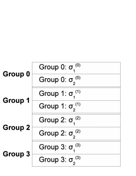
Figure 5: Illustration for Lemma 4.1

We now argue that the above coloring is perfect. First consider the case where $p\geq 6$. Let $c$ be any color and let $j$ be the group to which it belongs. The color $c$ appears in the once each in the rows $2j$ and $2j+1$. Let $l_{1},r_{1},u_{1}$ and $d_{1}$ be the colors appearing in the left, right, up and down positions of $c$ appearing the first row, respectively. Similarly, let $l_{1},r_{2},u_{2}$ be the colors in the neighboring positions of $c$ appearing in the second row. Of the eight neighboring colors, six of them ($l_{1},r_{1},d_{1},l_{2},r_{2}$ and $u_{2}$) belong to the same color group as $c$. By the niceness property ensured by Lemma A.1, all these six colors are distinct. The color $u_{1}$ belongs to the color group given by $(j-1)$ (modulo $p/2$). similarly, the color $d_{2}$ belongs to the color group given by $(j+1)$ (modulo $p/2$). Since $p\geq 6$, $j$, $(j-1)$ and $(j+1)$ are all different color groups. This shows that $u_{1}$ and $d_{1}$ are different, and they are also distinct from the above six other neighbors.

Let us consider the case of $p=4$. The issue here is that the number of groups is only two and so, for any color $c$, the $u_{1}$ and $d_{2}$ neighbors will belong to the same group. Nevertheless, we argue below that these two are distinct. Going through the proof of Lemma A.1, we see that it applies the same construction on any given set of elements $q$ elements $\Omega$. Therefore, for any color $c$ belonging to group $0$ and $c^{\prime}$ belonging to group $1$, if $c$ and $c^{\prime}$ appear in the same positions under first set of permutations ($\sigma^{(0)}_{1}$ and $\sigma^{(1)}_{1}$) then they also appear in the same position under the second set of permutations ($\sigma^{(0)}_{2}$ and $\sigma^{(1)}_{2}$). Based on the property, we now argue that the coloring scheme is perfect. Refer to Figure 6 for an illustration. Let $c$ be any color from the group $0$. Consider the $u_{1}$ and $d_{2}$ neighbors of $c$. Let $y_{1}$ and $y_{2}$ be the positions in which $c$ appears in the permutations $\sigma^{(0)}_{1}$ and $\sigma^{(1)}_{2}$, respectively. Then, $u_{1}=\sigma^{(1)}_{2}(y_{1})$ and $d_{2}=\sigma^{(1)}_{1}(y_{2})$. Let $c^{\prime}=\sigma^{(1)}_{1}(y_{1})$. By the property stated above, $\sigma^{(1)}_{2}(y_{2})$ is also $c^{\prime}$. Notice that $u_{1}$ and $d_{2}$ are the up and down neighbors of $c^{\prime}$. By the properties of nice permutations, these are distinct. A similar argument applies for the case of colors in group 1. $\Box$

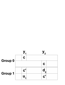
Figure 6: Illustration for Lemma 4.1

Nice Permutations (Proof of Lemma A.1)

Without loss of generality, assume that $\Omega=\{0,1,2,\ldots,q-1\}$. We define $\sigma_{1}$ to be the identity permutation: for $0\leq i<q$, $\sigma(i)=i$. The permutation $\sigma_{2}$ is defined as follows: for $0\leq i<q$, $\sigma_{2}(i)=5i+2\pmod{q}$. It is easy to see that $\sigma_{2}$ is indeed a permutation (because $5$ is a prime number and so, it is a generator for $Z_{q}$ – the additive group modulo $q$). We proceed argue that $\sigma_{1}$ and $\sigma_{2}$ form a nice pair. Throughout the discussion below all calculations are performed modulo $q$.

Consider any element $0\leq a<q$. Five of its neighbors are:

$l_{1}=a-1$	$r_{1}=a+1$	$d=5a+2$
$l_{2}=a-5$	$r_{2}=a+5$

where all the above calculations are performed modulo $q$. We will consider the sixth up-neighbor $u$ later. It is easy to see that $l_{1},r_{1},l_{2}$ and $r_{2}$ are all distinct (because $q\geq 8$ and so, $-1,+1,-5$ and $+5$ are all distinct modulo $q$). We next argue that $5a+2$ is distinct from the other four numbers. For an element $0\leq i\leq q$, let $g(i)$ be the set generated by $i$, i.e., $g(i)=\{ix\pmod{q}~{}:~{}x\geq 1\}$. Now, by contradiction, suppose, $5a+2=a+\delta$, for some $\delta\in\{-1,+1,-5,+5\}$. This implies that $4a+2=\delta$. Notice that $4a+2\in g(2)$, but $\delta\not\in g(2)$, (because $q$ is an even number and $q\geq 8$). This shows that $5a+2$ is distinct from the other four numbers.

We next prove that the up-neighbor $u$ is different from the other five neighbors. Let us first consider the case of $l_{1}$. Notice that the down-neighbor of $l_{1}$ is $5(a-1)+2$ and $5(a-1)+2\neq a$ (because $q$ is an even number and so, $3\not\in g(4)$). This means that the down-neighbor of $l_{1}$ is not $a$. On the other hand, the down-neighbor of $u$ is $a$. Therefore, we get that $l_{1}\neq u$. A similar argument shows that $r_{1}\neq u$. Let us now consider the case of $l_{2}$. Notice that $a=\sigma_{2}(u)$ and so, $l_{2}=5u-3$. It is easy to see that $5u-3\neq u$ (because $3\not\in g(4)$). This shows that $l_{2}\neq u$. A similar argument shows that $r_{2}\neq u$. Finally, let us show that $d\neq u$. To prove the claim, it suffices to show that the down-neighbor of $d$ is not $a$. The down-neighbor $d$ is $5d+2=5(5a+2)+2=25a+12$. We see that $25a+12\neq a$ (because $q$ is a power of two and so, $-12\not\in g(24)$). $\Box$

Appendix B Middle L-hop Issue

As mentioned in Section 5.3 regarding Halo pattern under indirect routitng, the middle L-hop poses an interested issue. This is discussed here.

The notion of congruence classes is useful in determining the load contributed by the middle L-hop. We say that two supernodes are congruent, if they are incident on the same set of nodes. Thus, the supernodes are portioned into as many congruence classes as there are nodes in a bucket. For example, in Figure 1(b), there are 16 congruence classes each containing two supernodes; supernodes $\{0,16\}$ belong to one congruence class, and $\{1,17\}$ belong to another. Two L-links going from nodes $u_{1}$ to $v_{1}$ and $u_{2}$ to $v_{2}$ are said to be congruent, if the same set of supernodes are incident on $u_{1}$ and $u_{2}$ and the same set of supernodes are incident on $v_{1}$ and $v_{2}$. For instance, in Figure 1(b), the L-links going from node $0$ to $8$, and the L-links going from node $16$ to $24$ in all the supernodes form a congruence class. The number of L-links in a congruence class is $n_{s}n_{d}$.

Middle L-hop: At a first glance, it may seem that how the $n_{s}$ blocks are mapped to the $n_{s}$ supernodes is not crucial. However, we argue that the above mapping is important and that it determines how the middle L-hop load is distributed over the L-links. Consider an L-link $e$ in supernode $a$ from node $u$ to a node $v$. There is a set of $h$ supernodes incident on the node $u$ and similarly, there is a set of $h$ supernodes incident on the node $v$. The link $e$ will be used as the middle L-hop whenever any data is sent from the former set of supernodes to the latter set of supernodes. This data will be striped over the $n_{s}n_{d}$ L-links in the congruence class of $e$. Let us analyze the case where this amount of data will be large. A block mapped to a supernode has four neighboring blocks mapped to four other supernodes; thus, each supernode can be viewed as having four neighboring supernodes. Now, unless the block-to-supernode mapping is done carefully, the set of supernodes incident on $u$ may find many of their neighboring supernodes being incident on the node $v$ causing link $e$ to receive a lot of data. To avoid the middle L-hop issue, the block-to-supernode mapping must ensure that the neighbors of any congruence class of supernodes are spread across the other congruency classes. A simple way to achieve the above goal is to map the blocks to supernodes in a random fashion. Notice that this method is the same as random supernode blocking scheme proposed by Bhatale et al. [5] (see Section 4.3). More sophisticated techniques, for instance based on mod-coloring, may provide better mapping schemes. This is left as future work.

Appendix C Transpose Pattern

C.1 Transpose Pattern : Direct Routing

Here we discuss the boundary cases mentioned in Section 4.4 and also present the derivations for the LL and LR link throughput for Transpose under direct routing.

We discussed that with respect to D-links throughput, both row-wise and column-wise mappings are equally good. However, two minor issues dealing with boundary cases distinguishes the two schemes. The first issue is regarding the LR-link throughput. Consider the case of row-wise mapping. Since we assume that $P$ is a power of two, each row will fit within a drawer (if $P\leq 32$), or it will span two drawers (if $P=64$) or it will span the entire supernode (if $P=128$). In the first case, there will be no load on the LR-link due to intra-supernode communication. In the second case, the load on any LR-link (due to intra-supernode communication) will be $(1/8)$ units; on the other hand, in the third case, the load will be $(1/16)$. This is because, in the second case only LR links connecting two pairs of drawers are used; whereas in the third case, LR links across all the four drawers are used. Hence, for the case where $P=64$ and $Q\neq 64$, the column-wise mapping will be better; similarly, for the case where $P\neq 64$ and $Q=64$, the row-wise mapping will be better. The second issue is regarding another boundary case. Both the schemes require that either $P$ or $Q$ is at most $128$. Thus, for the grid of size $128\times 256$, we must choose column-wise mapping and similarly, for the grid of size $256\times 128$, we must choose row-wise mapping. Based on the above discussions, it is easy to design a simple hybrid scheme which choose between row-wise and column-wise mapping based on the input grid dimensions.

Let us compute the LR-link throughput of the above hybrid scheme. Consider an LR-link $e$ going from a node $u$ to a node $v$ in some supernode $a$. Let us first focus on inter-supernode communication, which uses paths of the form L-D-L. Node $u$ has four processors each sending approximately $(1/2)$ units of data to its neighbors uniformly distributed across the other supernodes. Thus, a total load of $2$ units is distributed over the $32$ L-links originating from $u$. So, the load on $e$ is approximately $1/16$ units while being used as the first L-hop. Similarly, node $v$ receives $2$ units of data over its $32$ L-links. Hence, the load on $e$ is approximately $1/16$ units while being used as the second L-hop. So, the load on the link $e$ is $(1/8)$. We already saw that the load on any LR-link due to intra-supernode communication is at most $(1/8)$. So, the total load on any LR-link $e$ is at most $(1/4)$. So, the LR-link throughput is at least $80$  GB/s.

Let us now analyze the case of LL-links. First consider intra-supernode communication. The load on LL-links will be maximum when each row (or column) fits within a drawer; in this case, the load can be shown to be $(1/2)$ units. So, the load on any LL-link due to intra-supernode communication is at most $(1/2)$ units. The load due to inter-supernode communication is $(1/8)$ (the same as LR). So, the total load on any LL-link is at most $5/8$ units. Therefore, the LL-link throughput is at least $134$  GB/s.

C.2 Transpose Pattern : Indirect Routing

In Section 5.4, we presented a brief overview of the mapping strategies for the transpose pattern under indirect routing. A detailed discussion is given below.

We first focus on the D-links. The properties of indirect routing ensure that the load will be inherently well-balanced on the D-links. We already saw that row-wise mapping and column-wise mapping provide good load reduction on the D-links. Let us analyze the D-link throughput for row-wise mapping. Let the input grid be of size $P\times Q$. Consider a D-link $e$ going from a supernode $a$ to a supernode $b$. The paths are of the form L-D-L-D-L and the link $e$ can be used either as the first D-hop or the second D-hop. As discussed in the context of direct routing (Section 4.4), $a$ sends $64/n_{s}$ units of data to every other supernode and so, the overall data sent from supernode $a$ is $64(n_{s}-1)/NS$. This data is striped over all the $n_{s}n_{d}$ D-links going out of $a$. So, the load on $e$ while being used as the first D-hop is $(64/n_{s}n_{d})(1-1/n_{s})$. The link $e$ is used as the second D-hop whenever $b$ receives data from other supernodes. Thus, the total load on $e$ is $\ell(e)=(128/n_{s}n_{d})(1-1/n_{s})$. The D-link throughput of the row-mapping $\pi$ is

$$\tau_{{\rm D}}(\pi)=\frac{n_{s}}{n_{s}-1}\times\frac{n_{s}n_{d}}{128}\times 4\times 10=\frac{n_{s}}{n_{s}-1}\times 10h\approx 10h.$$

Now let us analyze the load on the L-links. First, consider the case of inter-supernode communication. Let $e$ be an L-link going from a node $u$ to a node $v$ in some supernode $a$. The paths in indirect routing are of the form L-D-L-D-L. The four processors in the node $u$ send approximately $(1/2)$ units of data to other supernodes. All this data is striped over all the D-links going out of the supernode $a$ and hence, the data is uniformly striped over the $32$ L-links going out from $u$. So, the load on the link $e$ being used as the first hop is approximately $(1/16)$. Similarly, the link $e$ will be used as the last L-hop, whenever $v$ receives data from other supernodes. A similar calculation shows that the load on $e$ while being used as the last hop is approximately $(1/16)$.

Let us now consider the case of middle L-hop. In contrast to the case of Halo (Section 5.3), our mapping ensures that the middle L-hop is not an issue. This is because, in Transpose, the amount of data sent from one supernode is another supernode is uniform across all the pairs of supernodes. Therefore, the amount of data sent between congruence classes of supernodes is uniform. As a result, all L-links get the same amount of load while being used as the middle L-hop. Let us explicitly compute the above quantity for the link $e$ going from $u$ to $v$ (in an intermediate supernode $a$). As we saw earlier, the amount of data sent from any supernode to any other supernode is $64/n_{s}$. Therefore, the amount of data sent from the supernodes incident on $u$ to the supernodes incident on $v$ is $h\times h\times 64/n_{s}$. All this data is striped over the $n_{s}n_{d}$ L-links in the congruence class of $e$. Therefore, the load on $e$ due to the middle L-hop is:

$$\frac{h\times h\times 64}{n_{s}}\times\frac{1}{n_{s}n_{d}}=\frac{n_{d}}{16}.$$

The total load on any L-link due to inter-supernode communication is $(1/16)+(1/16)+(n_{d}/16)=(2+n_{d})/16$. We saw that the load on LR and LL links (Section 4.4) due to intra-supernode communication is at most $(1/8)$ and $(1/2)$ units, respectively. Therefore, the total load on LR and LL links is at most $(4+n_{d})/16$ and $(10+n_{d})/16$, respectively. The throughput can be calculated automatically:

$$\tau_{{\rm LR}}(\pi) \geq \frac{320}{4+n_{d}}$$

$$\tau_{{\rm LL}}(\pi) \geq \frac{1344}{10+n_{d}}$$

The overall throughput is $\tau(\pi)\geq\min\{10h,320/(4+n_{d})\}$.

References

- [1] T. Agarwal, A. Sharma, A. Laxmikant, and L. Kalé. Topology-aware task mapping for reducing communication contention on large parallel machines. In IPDPS, 2006.
- [2] L. Arimilli, S. Baumgartner, S. Clark, D. Dreps, D. Siljenberg, and A. Maki. The IBM POWER7 HUB Module: A Terabyte Interconnect Switch for High-Performance Computer Systems. In Hot Chips, 2011.
- [3] L. Arimilli et al. The PERCS High-Performance Interconnect. In Symp. on High-Performance Interconnects, 2011.
- [4] K. Barker et al. On the Feasibility of Optical Circuit Switching for High-Performance Computing Systems. In SuperComputing, 2005.
- [5] A. Bhatele, N. Jain, W. Gropp, and L. Kale. Avoiding hot-spots on two-level direct networks. In SC, 2011.
- [6] R. Bianchinni and J. Shen. Interprocessor traffic scheduling algorithm for multiple-processor networks. IEEE Transactions on Computers, 36:396–409, 1987.
- [7] J. Dongarra and P. Luszczek. Introduction to the HPCChallenge Benchmark Suite. Technical report, ICL Technical Report, 10 2005. ICL-UT-05-01.
- [8] P. Ercal, J. Ramanujam, and P. Sadayappan. Task allocation onto a hypercube by recursive mincut bipartitioning. In Third Conference on Hypercube Concurrent Computers and Applications, 1988.
- [9] Z. Fang, X. Li, and L. Ni. On the communication complexity of generalized 2-d convolution on array processors. IEEE Transactions on Computers, 38:184–194, 1989.
- [10] Graph500. http://www.graph500.org/, 2011.
- [11] IBM Power 775 Supercomputer. http://www-03.ibm.com/systems/power/hardware/775/, 2011.
- [12] J. Kim, W. Dally, S. Scott, and D. Abts. Technology-driven, highly-scalable dragonfly topology. SIGARCH Comput. Archit. News, 36:77–88, 2008.
- [13] J. Michalakes, J. Dudhia, D. Gill, T. Henderson, J. Klemp, W. Skamarock, and W. Wang. The Weather Research and Forecast model: Software Architecture and Performance. In 11th ECMWF workshop on the use of High Performance Computing in Meteorology, 2004.
- [14] R. Rajamony, L. Arimilli, and K. Gildea. PERCS: The IBM POWER7-IH high-performance computing system. IBM Journal of Research and Development, 55(3):3, 2011.
- [15] B. Sinharoy et al. The IBM POWER7 Multicore Server Processor. IBM Journal of Research and Development, 55(3):1, 2011.
- [16] G. Zheng, G.Kakulapati, and L. Kale. Bigsim: A parallel simulator for performance prediction of extremely large parallel machines. In IPDPS, 2004.