Multiple Testing for Exploratory Research

Abstract

Motivated by the practice of exploratory research, we formulate an approach to multiple testing that reverses the conventional roles of the user and the multiple testing procedure. Traditionally, the user chooses the error criterion, and the procedure the resulting rejected set. Instead, we propose to let the user choose the rejected set freely, and to let the multiple testing procedure return a confidence statement on the number of false rejections incurred. In our approach, such confidence statements are simultaneous for all choices of the rejected set, so that post hoc selection of the rejected set does not compromise their validity. The proposed reversal of roles requires nothing more than a review of the familiar closed testing procedure, but with a focus on the non-consonant rejections that this procedure makes. We suggest several shortcuts to avoid the computational problems associated with closed testing.

T1Discussed in d10.1214/11-STS356A, d10.1214/11-STS356B and d10.1214/11-STS356C; rejoinder at r10.1214/11-STS356REJ.

and

1 Introduction

Central to the practice of statistics is the distinction between exploratory and confirmatory data analysis, and the interplay between the two. Exploratory data analysis suggests and formulates hypotheses, which can subsequently be rigorouslytested by confirmatory data analysis. The two types of data analysis require very different methods (Tukey, 1980): where confirmatory data analysis is structured and rigorous, exploratory data analysis can be open-minded and speculative.

Hypothesis testing and strict Type I error control are traditionally part of the realm of confirmatory data analysis, and, by implication, so are multiple testing procedures. However, multiple hypothesis testing is increasingly finding its way into exploratory data analysis. In genomics research, for example, typical experiments test thousands of hypotheses corresponding to as many molecular markers. Although somewhat structured, such experi-ments should be viewed as exploratory rather than as confirmatory. The collection of tested hypotheses is usually not selected on the basis of any theory, but because it is convenient and exhaustive. The rejected hypotheses are generally not meant to be reported as end results, but are to be followed up by independent validation experiments.

Despite the exploratory nature of these experiments, researchers do feel a need for multiple hypothesis testing methods and, in fact, routinely apply them. The main reason for this is that researchers want to protect themselves from following up on too many false leads and doing too many unsuccessful validation experiments. Most multiple testing methods, however, have been designed for confirmatory data analysis and are ill-suited for the specific requirements of exploratory research.

Before we come to the main argument of this paper, we would like to set the scene by sketching the requirements for an inferential procedure for exploratory research. Imagine the situation that we are exploring a large, but finite number of candidate hypotheses, indiscriminately selected. Rather than rigorously proving the validity of some or all of these hypotheses, as in confirmatory analysis, we want to select a number of promising hypotheses for further probing in a next phase of validation. The open-minded nature of exploratory research can be described by three characteristics: exploratory research is mild, flexible and post hoc. We explain these three terms below, contrasting them with the more familiar characteristics of confirmatory research.

An inferential procedure is mild if it allows some false positives among the selected hypotheses. This is the most obvious characteristic of exploratory research. Mildness is reasonable because false positives are expected to be detected and removed in later validation experiments. Confirmatory research, in contrast, being the final phase of the research cycle, is not mild but strict.

An inferential procedure is flexible if it does not prescribe to the researcher which precise hypotheses to select or not to select. For example, if the procedure ranks the hypotheses from most to least promising, but the researcher detects a commontheme in the hypotheses ranked second, third and fourth, he or she can choose to follow up on these three hypotheses and disregard the hypothesis that ranked first. In fact, the researcher may also choose to follow up on the hypothesis that ranked last, if that fits the same theme. Such freedom, “picking and choosing,” is an important part of the hypothesis-generating aspect of exploratory research. In confirmatory research, in contrast, selection of an interesting and coherent collection of hypotheses has been done prior to the experiment, so that flexible selection is not necessary.

Finally, an inferential procedure is post hoc if it allows all choices that are inherent to the procedure to be made after seeing the data. Specifically, how mild the procedure should be, and which precise set of hypotheses to select does not have to be chosen beforehand, but may be chosen on the basis of the data. This is probably the most distinguishing feature of exploratory research. The decision which inferences, and how many, to follow up is often based on a mixture of considerations; these considerations are usually not purely statistical, and are often difficult to make explicit. In contrast, in pure confirmatory research all choices regarding the testing procedure have to be set in stone before data collection.

An ideal multiple hypothesis testing procedure for exploratory research should sanction a mild, post hoc and flexible approach. Multiple testing procedures generally do not fulfil these criteria. The main present distinction is between multiple testing methods based on the familywise error (FWER), and variants, and methods based on the false discovery rate (FDR), and variants of that.

FWER-based methods control the probability of making any false rejection at a prespecified rate. These are the archetypical methods for confirmatory analysis. Such methods are clearly not mild, and they are not post hoc, as all data analysis decisions have to be made before seeing the data. They can be argued to be flexible in a limited sense: it is possible to refrain from rejecting some of the rejected hypotheses without violating control of the familywise error, but it is not possible to reject any hypotheses that were not selected by the procedure. A variant of familywise error, $k$-FWER, has been formulated that controls the probability of making at least $k\geq 1$ false rejections (Romano and Wolf, 2007). Depending on $k$, methods with this error rate are mild and are flexible in the same limited way as FWER itself is. Still, $k$-FWER-based methods have so far only attracted theoretical interest as in these methods value of $k$ may not be chosen post hoc, and nobody knows how to choose $k$ a priori in an applied setting. A recent permutation method of Meinshausen (2006) can be seen as a method that controls $k$-FWER simultaneously for all values of $k$, and consequently allows post hoc selection of $k$. This method is mild, post hoc, and quite flexible, although it does not allow a fully arbitrary selection of the set of rejected hypotheses.

False Discovery Rate (Benjamini and Hochberg, 1995) methods control the expected proportion of falsely rejected hypotheses among the rejected hypotheses. Such methods are not very well suited for traditional confirmatory research and take a step toward exploratory research. FDR-based methods are certainly mild compared to FWER-based methods. However, they are not post hoc, as the set of rejected hypotheses is completely determined after setting the FDR threshold. Moreover, FDR-based methods are not flexible: as shown by Finner and Roters (2001), and illustrated in a practical example by Marenne et al. (2009), selecting a subset from the hypotheses that the FDR-controlling procedure rejects may increase the false discovery rate above the prespecified level, just like, of course, selecting a superset can. Many variants of FDR have been proposed (e.g., Storey, 2002; Efron et al., 2001; Van Der Laan, Dudoit and Pollard, 2004), but none of these has the desired three characteristics of the ideal multiple testing procedure for exploratory inference. Methods have been formulated for selective inference (Benjamini and Yekutieli, 2005), but these still do not allow the full flexibility of exploratory selection.

In this paper we present an approach to multiple testing that does allow mild, flexible and post hoc inference. By the nature of the requirements of being flexible and post hoc, such a procedure cannot prescribe what hypotheses to reject, but can only advise. This reverses the traditional roles of the user and the procedure in multiple testing. Rather than, as in FWER- or FDR-based methods, to let the user choose the quality criterion, and to let the procedure return the collection of rejected hypotheses, the user chooses the collection of rejected hypotheses freely, and the multiple testing procedure returns the associated quality criterion. In our view, the task of a multiple testing procedure in the exploratory context is not to dictate what to reject, but to quantify the risk taken, in terms of the potential number of false rejections, of following up on any specific set of hypotheses, chosen freely.

This reversal of roles can be achieved while avoiding the pitfall of proposing yet another variant of FWER or FDR; it can be done simply by combining the familiar concept of the confidence set, the discrete version of the confidence interval, with the well-known closed testing procedure (Marcus, Peritz and Gabriel, 1976), widely recognized as a fundamental principle of multiple testing. What we will show is that the closed testing procedure can be used to construct exact simultaneous confidence sets for the number of false rejections incurred when rejecting any specific set of hypotheses, measuring the risk of following up on this particular set of hypotheses. Because the confidence sets are simultaneous over all possible sets of rejected hypotheses, the user is free to optimize, making the procedure valid even under post hoc selection of the rejected set.

The approach we propose is constrained by the requirement that the number of hypotheses potentially to be followed up is finite and that these hypotheses can be listed a priori. While this requirement rules out the most open-minded and unstructured applications of exploratory research, many exploratory problems are structured enough to fit the framework.

Our proposed procedure has strong links to $k$-FWER methods. In fact, the constructed confidence sets can be seen as controlling the $k$-FWER, but simultaneously for all values of $k$, thus sanctioning post hoc selection of $k$ and removing the requirement of selecting $k$ a priori, which traditionally plagues $k$-FWER-based methods. Through this, our method links to the approach of Meinshausen (2006); we come back to this link in Section 4.2.

Another interesting link is with methods that have appeared in recent years for estimating $\pi_{0}$, the number of true hypotheses among the collection of all hypotheses (Schweder and Spjøtvoll, 1982; Benjamini and Hochberg, 2000; Langaas, Lindqvist and Ferkingstad, 2005; Meinshausen and Bühlmann, 2005; Jin and Cai, 2007). The procedure outlined in this paper automatically gives a confidence set for the quantity $\pi_{0}$, because the collection of all hypotheses is one of the possible sets of rejected hypotheses that the user can choose to follow up, and the number of false rejections in that set is exactly $\pi_{0}$.

The outline of this paper is as follows. In the next section, we review the closed testing procedure and the role of the concept of consonance in that procedure. We argue that non-consonant closed testing procedures have been underrated, and illustrate the type of additional inference that is possible from a non-consonant closed testing procedure, but typically neglected, before we argue how these additional inferences can be used to construct a confidence set. Section 3 applies the approach to selection of variables in a multiple regression model. Section 4 explores computational issues related to closed testing procedures and proposes situations in which shortcuts can be found. Finally, Section 5 looks at estimation of the number of correctly rejected hypotheses. Software to perform the methods described in this paper is available in the cherry package, downloadable from CRAN.

2 Non-consonant Closed Testing

The closed testing procedure (Marcus, Peritz and Gabriel, 1976) is well known as a cornerstone of familywise error control. In this section we show how closed testing may also be used to construct confidence sets for the number of falsely rejected hypotheses.

First we introduce some notation. Let $H_{1},\ldots,H_{n}$ be the collection of hypotheses of interest, the elementary hypotheses, out of which we want to select hypotheses to follow up. Some of these hypotheses are true; let $T\subseteq\{1,\ldots,n\}$ denote the unknown indices of true hypotheses. To use a closed testing procedure, we must consider not only the elementary hypotheses, but also all intersection hypotheses of the form $H_{I}=\bigcap_{i\in I}H_{i}$, where $I\subseteq\{1,\ldots,n\}$, $I\neq\varnothing$. Figure 1 illustrates the intersection hypotheses formed by three hypotheses $H_{1}$, $H_{2}$ and $H_{3}$ in the form of a graph, with arrows denoting subset relationships (ignore the crosses for now).

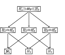
Figure 1: Intersection hypotheses formed by elementary hypotheses $H_{1}$, $H_{2}$ and $H_{3}$. Rejected hypotheses have been marked with a cross. The rejection of $H_{2}\cap H_{3}$ is a non-consonant rejection.

An intersection hypothesis $H_{I}$ is true whenever all $H_{i}$, $i\in I$, are true, that is, whenever $I\subseteq T$. Let the closure $\mathcal{C}$ be the collection of all nonempty subsets of the index set $\{1,\ldots,n\}$. Each element of $\mathcal{C}$ corresponds to an intersection hypothesis, some of which are true. Let $\mathcal{T}=\{I\in\mathcal{C}\dvtx I\subseteq T\}$ be the subsets corresponding to true intersection hypotheses. The collection $\mathcal{C}$ also contains singleton sets. Noting that we can equate $H_{i}=H_{\{i\}}$, let $\mathcal{H}=\{I\in\mathcal{C}\dvtx\#I=1\}$ be the subsets corresponding to the elementary hypotheses.

The closed testing procedure works as follows. It requires $\alpha$-level tests for every intersection hypothesis $H_{I}$, $I\in\mathcal{C}$, which are called the local tests. Applying these local tests, let $\mathcal{U}\subseteq\mathcal{C}$ be the collection of subsets $U\in\mathcal{C}$ for which the test rejects the hypotheses $H_{U}$. The collection $\mathcal{U}$ represents the raw rejections uncorrected for multiple testing. Based on these raw rejections, the closed testing procedure rejects every $I\in\mathcal{C}$ for which $J\in\mathcal{U}$ for every $J\supseteq I$. Denote the collection of all such $I$ by $\mathcal{X}$. It was shown very elegantly by Marcus, Peritz and Gabriel (1976) that with this rejected set the closed testing procedure strongly controls the familywise error for all hypotheses $H_{I}$, $I\in\mathcal{C}$, at level $\alpha$. They showed that the event $E=\{H_{T}\notin\mathcal{U}\}$, which happens with probability at least $1-\alpha$, implies that $\mathcal{X}\cap\mathcal{T}=\varnothing$.

In the example of Figure 1, suppose that the hypotheses rejected by the local tests are the ones marked with a cross. In this example $H_{1}$ is rejected by the closed testing procedure because the four hypotheses $H_{1}$, $H_{1}\cap H_{2}$, $H_{1}\cap H_{3}$ and $H_{1}\cap H_{2}\cap H_{3}$ are all rejected by their local test. In fact, in the example of Figure 1 we have $\mathcal{X}=\mathcal{U}$, because each hypothesis rejected by the local test has all its ancestors in the graph of Figure 1 rejected.

When using the closed testing procedure for familywise error control, the intersection hypotheses are generally constructed for the benefit of the procedure, but are not of genuine interest by themselves. The reported result of the procedure is therefore usually not the collection $\mathcal{X}$, but only $\mathcal{X}\cap\mathcal{H}$. From the perspective of familywise error control, a rejection $I\in\mathcal{X}$ for which there is no $J\in\mathcal{X}\cap\mathcal{H}$ with $J\subset I$ is a wasted rejection. Such a rejection was not instrumental in facilitating a rejection of interest; if that rejection had not occurred, the same rejected set $\mathcal{X}\cap\mathcal{H}$ of elementary hypotheses would have resulted from the procedure. This consideration has led to a quest for consonant closed testing procedures. A closed testing procedure is consonant if the local tests for every $I\in\mathcal{C}$ are chosen in such a way that rejection of $I$ implies rejection of at least one $J\in\mathcal{H}$. It is easily shown that for every closed testing procedure there is a consonant procedure that rejects at least as much in $\mathcal{X}\cap\mathcal{H}$. Moving from a non-consonant to a consonant procedure may often lead to a gain in power on the elementary hypotheses. From a familywise error perspective, consonance is, therefore, a desirable property, and non-consonant procedures are best avoided (Bittman et al., 2009).

However, once we are interested in milder inference than a familywise error-based one, the premise that only rejection of the elementary hypotheses $H_{1},\allowbreak\ldots,H_{n}$ is of interest should be dropped, and non-consonant closed testing procedures need not beavoided. We illustrate this with the simple example of Figure 1, which will immediately serve as a small showcase of the point of view on multiple testing we propose in this paper. Here, the only one of the elementary hypotheses that has been rejected is $H_{1}$. Of the intersection hypotheses we see three “consonant” rejections, namely $H_{1}\cap H_{2}\cap H_{3}$, $H_{1}\cap H_{2}$ and $H_{1}\cap H_{3}$, which have all facilitated rejection of the elemental hypothesis $H_{1}$. We also see one “non-consonant” rejection, $H_{2}\cap H_{3}$. A familywise error perspective would dictate rejection of $H_{1}$ and nothing else. An exploratory perspective, however, on the same data would lay the choice what and how many hypotheses to reject with the user. An obstinate user could, for example, choose not to reject $H_{1}$, but to reject $H_{2}$ and $H_{3}$. What can we say about the risk incurred by such a user in terms of the number of false rejections?

In general, the number of false rejections made when rejecting the hypotheses $H_{i}$, $i\in R$, is equal to $\tau(R)=\#(T\cap R)$, the number of true null hypotheses among $R$. For a given set $R$, this quantity is just a function of the model parameters, for which we can find estimates and confidence intervals just like for any other function of the model parameters. The confidence interval takes the form of a confidence set, because $\tau(R)$ only takes discrete values. We come to the issue of estimation later, and first construct such a confidence set.

To construct a confidence set, define

$$\mathcal{C}_{R}=\{I\in\mathcal{C}\dvtx I\subseteq R\},$$

the collection of all intersection hypotheses involving only rejected hypotheses, and let

$$t_{\alpha}(R)=\max\{\#I\dvtx I\in\mathcal{C}_{R},I\notin\mathcal{X}\},$$

taking $t_{\alpha}(R)=0$ if $\mathcal{C}_{R}\subseteq\mathcal{X}$. The quantity $t_{\alpha}(R)$ is the size of the largest subset of $R$ for which the corresponding intersection hypothesis is not rejected by the closed testing procedure. We claim that the set

$$\{0,\ldots,t_{\alpha}(R)\}$$ (1)

is a $(1-\alpha)$-confidence set of the parameter $\tau(R)$.

To prove the coverage of this set, remember that if the event $E$ has happened, then all rejections that the closed testing procedure has made are correct. Given that $E$ has happened, the value of $\tau(R)$ cannot be greater than the value of $t_{\alpha}(R)$, because otherwise a true intersection hypothesis would have been rejected, which is inconsistent with the definition of $E$. Consequently, $\tau(R)\in\{0,\ldots,t_{\alpha}(R)\}$ with probability at least $\mathrm{P}(E)\!=\!1\!-\!\alpha$, which makes $\{0,\ldots,\allowbreak t_{\alpha}(R)\}$ a $(1-\alpha)$-confidence set for $\tau(R)$.

The confidence set (1) is always one-sided, never providing a nontrivial lower bound for $\tau(R)$. The reason for this is that the confidence set originates from a procedure that is focused on rejecting, not on accepting null hypotheses. Furthermore, for many applications the null hypotheses are point hypotheses, of which it can never be proved that they are true. In these cases, no procedure can produce a confidence interval with a nontrivial lower bound, and the upper bound is the only bound of real interest.

Often interest is in quantifying not the number of true hypotheses in $R$, but the number of false hypotheses $\phi(R)=\#R-\tau(R)$. A confidence set for $\phi(R)$ follows from (1) immediately as

$$\{f_{\alpha}(R),\ldots,\#R\},$$

where $f_{\alpha}(R)=\#R-t_{\alpha}(R)$. Confidence sets for other quantities that depend only on $\tau(R)$ and $\#R$, such as the false discovery proportion $\tau(R)/\#R$, may be derived in a similar way.

Returning to the example of Figure 1 with choice of a rejected set, $R=\{2,3\}$, we have a realized value of $t_{\alpha}(R)=1$. We conclude that $\{0,1\}$ is a $(1-\alpha)$-confidence set for the number of false rejections incurred when rejecting $H_{2}$ and $H_{3}$. Even though neither $H_{2}$ or $H_{3}$ was rejected by the closed testing procedure, when rejecting both $H_{2}$ and $H_{3}$ the user can be confident of making at least one correct rejection. The choice of $R=\{2,3\}$ is only one of many possible rejection choices that the user can make. For each alternative choice, a confidence set can be made in the same way as for $R=\{2,3\}$. These confidence sets, and the corresponding confidence sets for $\phi(R)$, are given in Table 1.

Table 1: Confidence sets for the numbers of incorrect rejections $\tau(R)$ and correct rejections $\phi(R)$ incurred with various choices of the rejected set, based on the closed testing result of Figure 1

$\bolds{R}$	Confidence set for $\bolds{\tau}\bolds{(R)}$	Confidence set for $\bolds{\phi}\bolds{(R)}$
$\{1\}$	{0}	{1}
$\{2\}$	{0, 1}	{0, 1}
$\{3\}$	{0, 1}	{0, 1}
$\{1,2\}$	{0, 1}	{1, 2}
$\{1,3\}$	{0, 1}	{1, 2}
$\{2,3\}$	{0, 1}	{1, 2}
$\{1,2,3\}$	{0, 1}	{2, 3}

The important thing to note about confidence sets of the form (1) is that they are simultaneous confidence sets, which all depend on exactly the same event $E$ for their coverage. Because these confidence sets are simultaneous, the user can review all these confidence sets, and select the rejected set $R$ that he or she likes best, while still keeping correct $1-\alpha$ coverage of the selected confidence set: under the event $E$, all confidence sets cover the true parameter simultaneously, and therefore, under the same event $E$, the selected confidence set covers the true parameter. Consequently, the selected confidence set has coverage of at least $\mathrm{P}(E)=1-\alpha$. The simultaneity of the sets makes their coverage robust against post hoc selection.

In the specific case of Table 1, the user might choose to follow up on all three hypotheses, which would give him or her confidence in at least two discoveries of a false null hypothesis. On the other hand, if sufficient funds are available for only two validation experiments, the user may choose to follow up on any two hypotheses, any pair giving confidence of obtaining at most one false positive.

Contrary to the application of closed testing for familywise error control, in terms of confidence sets non-consonant rejections do improve the results obtained from the procedure. Without the rejection of $H_{2}\cap H_{3}$ in Figure 1 the confidence sets for $R=\{2,3\}$ and for $R=\{1,2,3\}$ would have been larger than the ones given in Table 1. From the definition of consonance it follows immediately that the value of $t_{\alpha}(R)$ in a consonant closed testing procedure is equal to the number of hypotheses in $R$ that are not rejected by the closed testing procedure under a familywise error regime. In non-consonant closed testing procedures, the value of $t_{\alpha}(R)$ can be substantially smaller, as we shall see in examples below.

Essentially, the example of Table 1 summarizes the confidence set approach to multiple testing. The user has unlimited options in selecting what to reject, and may review all options and their consequences in order to make his or her choice. This approach fulfills all three criteria set for multiple testing in exploratory research formulated in the introduction. The procedure is flexible, because it does not prescribe any rejections but leaves the choice which hypotheses to follow up completely in the hands of the user. The procedure is mild, because it allows any number or proportion of false rejections that the user desires. Furthermore, the procedure is post hoc, because it allows the user to review the consequences, in terms of the potential number of false rejections, of any choice of rejected hypotheses before making a final choice, without compromising the quality of the inferences obtained. Still, even with the lenience of all these properties, the inferential statements resulting from the procedure are absolutely classical and rigorous, requiring no new definitions of error rates but only the classical concept of simultaneous confidence sets.

3 Example: Selecting Covariates in Regression

One area of statistics in which common practice is highly exploratory and post hoc is the selection of covariates in a multiple regression. Methods such as forward or backward selection, or their combination, are typically used to select a model containing a subset of a set of candidate covariates. Often, $p$-values that are reported for the selected covariates completely ignore the selection process. The confidence set method outlined in the previous section can be used in this situation to set confidence limits to the number of selected variables that is truly associated with the response variable.

As an example, consider the physical dataset (Larner, 1996), in which 10 physical measurements on 22 male subjects (length, and circumference of various parts of the body) are used as covariates for modeling body mass. An analysis based on a linear regression model with a forward–backward algorithm selects the four covariates forearm, waist, height and thigh as the relevant variables. Table 2 gives the $p$-values of the covariates in both the full and the selected model. The reported $p$-values of the selected model are known to be anti-conservative as they do not take the selection into account. An important question to ask, therefore, is how many truly relevant variables are, in fact, included in this selection. This would give a measure of confidence for the selected set.

Table 2: Uncorrected $p$-values ($t$-test) for relevance of variables in the full model and selected model

Covariate	Full model	Selected model
(Intercept)	0.036	0.000
Forearm	0.061	0.000
Biceps	0.755	–
Chest	0.420	–
Neck	0.518	–
Shoulder	0.905	–
Waist	0.000	0.000
Height	0.033	0.005
Calf	0.303	–
Thigh	0.351	0.036
Head	0.105	–

Following the strategy outlined in the previous section, we construct a linear regression model with an intercept and 10 regression coefficients $\beta_{1},\ldots,\beta_{10}$, and define the elementary hypotheses $H_{i}$, $i=1,\ldots,\allowbreak 10$, to be the hypotheses that the corresponding regression coefficient $\beta_{i}=0$. Next we construct all 1,023 intersection hypotheses $H_{I}$, $I\in\mathcal{C}$, each of which corresponds to the hypothesis that $\beta_{j}=0$ for all $j\in I$. As the local tests we choose the $F$-test of the corresponding null model against the saturated model, tested at level $\alpha=0.05$.

The closed testing procedure rejects 626 out of the 1023 hypotheses, among which there is one elementary hypothesis: waist. Several non-consonant rejections have occurred. We can summarize these by finding the defining rejections, that is, the rejections $I\in\mathcal{X}$ which have no rejected subset $J\subset I$, $J\in\mathcal{X}$. For this dataset, these defining rejections are the following seven sets:

{waist}

{forearm, neck, shoulder, height}

{forearm, biceps, shoulder, calf}

{forearm, shoulder, height, calf}

{forearm, biceps, chest, neck, shoulder, thigh}

{forearm, shoulder, height, thigh}

{forearm, calf, thigh}

As each of these sets corresponds to a rejected intersection hypothesis, we can conclude with 95% confidence that each of the seven sets contains at least one truly relevant covariate. It is tempting to say that, beside waist, forearm must be relevant, since it is included in all defining sets except the first. This is not warranted, however, as the sets are also consistent with alternative truths, such as that both shoulder and thigh are relevant variables. What we can conclude, is that if we select, for example, the set

$$R=\{\mbox{waist, forearm, calf, thigh}\}$$ (2)

we have selected at least two relevant variables. Furthermore, we can also directly conclude that waist is a relevant variable.

Coming back to the set $R=\{\mbox{waist},\ \mbox{forearm},\break\mbox{height},\ \mbox{thigh}\}$ selected by the forward–backward procedure, we can find all 15 intersection hypotheses of the four hypotheses in $R$ and check whether they were rejected by the closed testing procedure. We find that $R\in\mathcal{X}$, but $\mbox{\{forearm, height, thigh\}}\notin\mathcal{X}$, so that $t_{\alpha}(R)=3$. Therefore, we can say with confidence that the selected set $R$ contains one truly relevant hypothesis, but not that it contains more than one. From this result, it is clear that the $p$-values given for the selected model in Table 2 are highly untrustworthy.

To find out how many of the original 10 hypotheses are relevant, we take $R$ to be the full set of 10 hypotheses, and we calculate $t_{\alpha}(R)=8$ for this set. Apparently, we can conclude that there are at least two covariates among these 10 that are determinants of mass. The smallest set that contains at least two relevant covariates is the set (2).

It should be noted that the set selected by variable selection procedure should not generally be expected to be optimal from a confidence set perspective, because the perspectives of the two procedures are quite different. This is best illustrated by thinking of a dataset in which there are two covariates which are both highly correlated with each other, and with the response. Variable selection algorithms will always choose one of the two variables, disregarding the second one as superfluous given the first. The confidence set approach, however, will emphasize the uncertainty of the choice between the two variables, and will not reject any intersection hypothesis that involves only one of the two covariates. To have confidence that at least one truly relevant covariate is included, both of the highly correlated variables must be selected. This reflects a difference in emphasis between the two approaches: variable selection selects optimal sets, whereas the confidence set approach quantifies the uncertainty inherent in the selection process.

It is interesting to investigate the price of post hoc selection relative to a priori selection. It is immediate from the procedure that reducing the tested set of hypotheses to a set $R$ a priori is at least as powerful as, and likely more powerful than, testing a larger set and selecting the same set $R$ post hoc. Post hoc selection will generally result in wider confidence sets than a priori selection: this is the price to be paid for the risk of overfit caused by post hoc selection. In the example this price is surprisingly small. If the set $R=\{\mbox{waist, forearm, height, thigh}\}$ would have been defined a priori as the set of hypotheses of interest, treating the remaining covariates’ regression coefficients as nuisance parameters, the confidence set of $\phi(R)$ improves from $\{1,2,3,4\}$ to $\{2,3,4\}$. The confidence set for $\phi(R)$ for the set $R$ defined in (2) does not change.

4 Shortcuts

In its standard form, application of a closed testing procedure requires $2^{n}-1$ tests to be performed. Smart bookkeeping can reduce this number somewhat, especially if some intersection hypotheses high up in the hierarchy turn out non-significant, because it can be used that if $I\notin\mathcal{X}$, then immediately $J\notin\mathcal{X}$ for every $J\subset I$, which saves calculation of some of the tests. Still, even with such tricks and with high computational power, the closed testing procedure becomes computationally intractable in its general form for a number of hypotheses around 20–30, depending on the computational effort needed for each single test.

If a large number of hypotheses is to be investigated, it is, therefore, convenient if the local tests can be chosen in such a way that not all these tests need to be calculated. Methods for avoiding calculation of some of the hypothesis tests in the closed testing procedure are known as shortcuts. The literature on shortcuts in the closed testing procedure has been focused mainly on consonant procedures, and on finding the rejected individual hypotheses (Grechanovsky and Hochberg, 1999; Zaykin et al., 2002; Hommel, Bretz and Maurer, 2007; Bittman et al., 2009; Brannath and Bretz, 2010). In this section, we loosely extend the concept of shortcuts to non-consonant procedures, and discuss ways of finding $t_{\alpha}(R)$ in a computationally easy way for specific choices of the local test, namely those based on Fisher combinations, on Simes’ inequality, and on sums of normally distributed test statistics. We also demonstrate how the permutation-based procedure of Meinshausen (2006) fits into the closed testing framework. Finally, we touch upon the possible use of other procedures than closed testing for constructing confidence sets.

4.1 Fisher Combinations

The case of independent null hypotheses deserves special attention as a benchmark, because several important multiple testing methods (Benjamini and Hochberg, 1995; Efron et al., 2001; Storey, 2002) have been initially formulated for independent hypotheses only. Independent tests are relatively rare in practical applications.

One highly suitable choice for the local tests in the independent case is Fisher’s combination method. It requires only the $p$-values $p_{1},\ldots,p_{n}$ of the tests of the elemental hypotheses $H_{1},\ldots,H_{n}$, and rejects an intersection hypothesis corresponding to $I\in\mathcal{C}$ whenever

$$-2\sum_{i\in I}\log(p_{i})\geq g_{\#I},$$

where $g_{r}$ is the $(1-\alpha)$-quantile of a $\chi^{2}$-distribution with $2r$ degrees of freedom. This test is a valid $\alpha$-level test of the hypothesis $H_{I}$ if the $p$-values $p_{i}$, $i\in I$, are independent. Note that the requirement of being a valid local test only refers to intersection null hypotheses that are true, so that there is no requirement of independence among $p$-values of false null hypotheses, nor even between $p$-values of true and false null hypotheses.

Table 3: Adverse events data, taken from Herson (2009), sorted to increasing $p$-values and with a typo corrected

Adverse event	$\bolds{p}$-value
Anemia	0.02
Myocardial infarct	0.03
Diarrhea	0.04
Nausea and vomiting	0.04
Stomatitis	0.08
Skin rash	0.10
Dehydration	0.12
Shortness of breath	0.18
Renal failure	0.20
Fever	0.23
Blurred vision	0.26
Nose bleed	0.28
Anorexia	0.30
Bronchitis	0.31
Wheezing	0.40
Headache	0.50

Fisher’s method is highly non-consonant, as sum test often are. Moreover, the simple structure of the local tests allows easy shortcuts to be formulated. For any $s<\#R$, we have that $t_{\alpha}(R)\leq s$ if

$$u(R,s+1)\geq\max_{0\leq j\leq M}\{g_{s+j+1}-u(\bar{R},j)\},$$

where $u(I,k)$ is the sum of the $k$ smallest values of $-2\log(p_{i})$ with $i\in I$, $\bar{R}$ is the complement of $R$, and $M$ is the number of values of $-2\log(p_{k})$ in $\bar{R}$ smaller than the $(s+1)$th largest value of $-2\log(p_{k})$ in $R$. This shortcut, related to the shortcut of Zaykin et al. (2002), allows calculation of $t_{\alpha}(R)$ for any $R$ without exponentially many tests having to be calculated. It is an example of a general method for finding shortcuts for exchangeable tests, which we explain in Appendix A.

As an example, consider the following application in the realm of adverse drug reactions. Consider the data in Table 3, which give raw $p$-values for null hypotheses concerning the presence of adverse drug reactions reported for a certain drug. We assume the hypotheses to be independent, although the validity of this assumption can be disputed.

An analysis based on familywise error rate (Šidák, 1967) or false discovery rate (procedure of Benjamini and Hochberg, 1995) results in no rejections for these data. However, among the hypotheses with small $p$-values, the researcher notices three hypotheses concerned with problems of the gastrointestinal tract: diarrhea, nausea and vomiting, and stomatitis. The researcher may hypothesize that the drug causes problems in this area, and may consider following up on these three hypotheses. For this choice of $R$ we can calculate $f_{\alpha}(R)=1$ at $\alpha=0.05$, and we can conclude that the drug in question has at least some adverse effect somewhere in the gastrointestinal tract. The researcher can be confident that following up on these three hypotheses will lead to at least one potentially successful validation experiment.

Figure 2: Number of correct rejections versus number of rejections for the data of Table 3. The bars only give the lower bound of the 95% confidence interval; the number of false null hypotheses (correct rejections) is likely to be larger than indicated.

Alternatively, if the researcher wants to optimize the number of correct rejections, he or she may simply wish to reject those hypotheses that have the smallest $p$-values. In that case the only choice the researcher has to make is the number of rejections, and a plot such as Figure 2 may be made, which plots the lower bound of the number of correct rejections $f_{\alpha}(R)$ against the number of rejections $\#R$. Based on this plot, the researcher can claim with 95% confidence that at least five adverse drug reactions occur for this drug, and that these are found among the hypotheses with the 10 smallest $p$-values. If the researcher does not have funds available for 10 follow-up experiments, the researcher may want to validate the top six, which gives confidence of finding at least four false null hypotheses, or perhaps the top three, for confidence of finding at least two false null hypotheses.

Figure 2 also illustrates the link between our proposed approach and the $k$-FWER criterion. A user wishing to control $k$-FWER can reject any set $R$ that has $t_{\alpha}(R)<k$, for example taking $R$ as the set corresponding to the $i$ smallest $p$-values, choosing $i$ as the largest value such that $t_{\alpha}(R)<k$ still holds. The graph of Figure 2 simultaneously shows the numbers of rejections allowed with $k=1,2,3,4,\ldots,$ which are given by $i=0,3,6,7,\ldots.$ A major advantage of our approach over traditional $k$-FWER control approaches is that control is simultaneous over all rejected sets, and therefore over all choices of $k$. The procedure thus bridges the gap between weak FWER control, related to $n$-FWER, and strong 1-FWER control. Furthermore, rather than choosing $k$ in advance, its value may be picked after seeing the data without destroying the associated control property. The link between $k$-FWER and our approach is not limited to local tests based on Fisher combinations.

An interesting feature of using Fisher’s method in combination with the confidence set approach is that the method may prove the presence of false null hypotheses even in the situation that no individual $p$-value is smaller than $\alpha$. Consider the following $p$-values, taken from Huang and Hsu (2007):

$$p_{1}=0.051;\quad p_{2}=0.064;$$

$$p_{3}=0.097;\quad p_{4}=0.108.$$

Even though all $p$-values are non-significant individually, the confidence set for $\phi(R)$ when rejecting the top two hypotheses is $\{1,2\}$, when rejecting the top three hypotheses $\{2,3\}$, and when rejecting all four hypotheses $\{2,3,4\}$. This indicates that even in absence of any individually significant hypotheses we can make a rigorous confidence statement that at least two out of the first three hypotheses are false.

Fisher’s method is highly non-consonant, and can be very powerful, especially if there are many moderately small $p$-values. It is not uniformly more powerful than other tests, however. Compared to consonant local tests, such as Sidak’s, Fisher’s method tends to have smaller values of $t_{\alpha}(R)$ for large rejected sets $R$ due to its large number of non-consonant rejections, but Sidak’s method often has more sets $R$ which have $t_{\alpha}(R)=0$, due to a higher number of consonant rejections.

4.2 Simes Type Local Tests and Permutations

A different type of local test with potentially non-consonant rejections is a type of test that rejects a hypothesis $H_{I}$, $I\in\mathcal{C}$, whenever

$$p^{I}_{(i)}\leq c^{\#I}_{i}$$ (3)

for at least one $1\leq i\leq\#I$, where $p^{I}_{(i)}$ is the $i$th smallest among the $p$-values $\{p_{j}\}_{j\in I}$ of the elementary hypotheses with indices in $I$, and $c_{i}^{m}$, $1\leq m\leq n$, $1\leq i\leq m$, are appropriately chosen critical values. Without loss of generality we can take $c^{m}_{i}\leq c_{j}^{m}$ if $i\leq j$.

We call local tests of the form (3) Simes type local tests because if we choose

$$c_{i}^{m}=\frac{i\alpha}{m},$$ (4)

the test based on (3) is a valid $\alpha$-level test of $H_{I}$ by Simes’ (1986) inequality. Simes’ inequality holds whenever $p$-values of true null hypotheses are independent, but also under more general conditions, as investigated by Sarkar (1998). In particular it holds for $p$-values from identically distributed, nonnegatively correlated test statistics.

A variant of Simes’ inequality has been proposed by Hommel (1983). This variant uses critical values

$$c_{i}^{m}=\frac{i\alpha}{K_{m}\cdot m},$$ (5)

where $K_{m}=\sum_{v=1}^{m}v^{-1}$. Unlike the one based on Simes’ inequality, the local test defined by these critical values is of the correct level $\alpha$ whatever the dependence structure of the original $p$-values.

Local tests of the form (3) do not generally allow shortcuts for the calculation of $t_{\alpha}(R)$, but two useful shortcuts are available if the critical values are chosen in such a way that

$$c_{i}^{l}\leq c_{i}^{m}\quad\mbox{whenever }l\geq m.$$ (6)

The first shortcut this condition allows is the general shortcut described in Appendix A, the conditions of which are fulfilled whenever (6) holds. The second shortcut is even faster to calculate, but is less general: it holds for rejected sets of the form $R=\{i\dvtx p_{i}\leq q\}$ only. Let $p_{(i)}$, $i=1,\ldots,n$, be short for $p_{(i)}^{I}$ with $I=\{1,\ldots,n\}$. For $R$ of the form mentioned, we have the shortcut

$$f_{\alpha}(R)>\max\{S_{r}\dvtx 1\leq r\leq\#R\},$$ (7)

where $S_{r}=\max\{s\geq 0\dvtx p_{(r)}\leq c^{n}_{r-s}\}$. The value of $S_{r}$ can be interpreted as the number of more stringent critical values $c^{n}_{r-1},\ldots,c^{n}_{1}$ by which the $p$-value $p_{(r)}$ overshoots its mark $c^{n}_{r}$. The number of false hypotheses is larger than the greatest such overshoot of the ordered $p$-values in the set $R$. The shortcut (7) is useful for making plots such as the one in Figure 2. We prove this shortcut in Appendix B. A slightly more powerful variant of the shortcut (7) is available if we have (6) and

$$c_{i}^{m}\geq c_{i-w}^{m-w}\quad\mbox{for every $1\leq w<i$.}$$ (8)

In this case, we have the same shortcut as (7), but with $S_{r}=\max\{s\geq 0\dvtx p_{(r)}\leq c^{n-s}_{r-s}\}$. The proof of this statement is analogous to the proof for (7) and is also given in Appendix B. It is easy but tedious to show that the Simes critical values (4) and (5) conform to (6) and that the critical values (4) also conform to (8), so that the shortcuts may be used for these choices of the local test (see also Benjamini and Heller, 2008).

As a side note, we remark that the critical values (4) and (5) are the same as the critical values used in the false discovery rate controlling algorithms of Benjamini and Hochberg (1995) and Benjamini and Yekutieli (2001), respectively. The correspondence between the critical values creates a connection between the corresponding methods. The set that has been rejected by the false discovery rate algorithm always has $f_{\alpha}(R)>0$ based on the closed testing procedure with the corresponding local test. Note that the assumptions underlying each local test and its corresponding false discovery rate algorithm are very similar. For the example data of Section 4.1, the Simes local test leads to no rejections, which is consistent with finding no rejections with the procedure of Benjamini and Hochberg (1995).

Permutation testing can be a powerful tool to take into account the joint distribution of the $p$-values. Useful shortcuts in a closed testing procedure with permutation-based local tests can be constructed from the work of Meinshausen and Bühlmann (2005) and Meinshausen (2006). These authors describea permutation-based way to find critical values $k_{i}$, $i=1,\ldots,n$, such that the probability under the complete null hypothesis that $p_{(i)}\leq k_{i}$ for at least one $i$ is bounded by $\alpha$. The same method may in principle also be used to find corresponding permutation critical values $k_{i}^{I}$ for every intersection hypothesis $H_{I}$, $I\in\mathcal{C}$, and therefore a local test for every intersection hypothesis $H_{I}$; a closed testing procedure can be made on the basis of these tests. However, unless the number of hypotheses is limited, this will be extremely time-consuming, and it would lead to a closed testing procedure for which shortcuts are not available. A way out of this dilemma can be found by remarking that, by construction of the permutation critical values, we have $k_{i}^{I}\geq k_{i}$ for every $i$ and $I$. Therefore, a valid, though conservative, local test may be constructed by simply using a procedure of the form (3) with $c_{i}^{m}=k_{i}$ for every $1\leq m\leq n$. This local test fulfils the condition (6) and therefore admits shortcuts. With this choice of a local test, the confidence set approach to multiple testing can be used for every collection of test statistics for which permutation is possible, opening up the possibility to use permutation-based closed testing in genomics research.

Meinshausen (2006) constructed simultaneous confidence bands for the number of falsely rejected hypotheses for rejected sets of the form $R=\{i\dvtx p_{i}\leq q\}$, similar to Figure 2, based on the permutation critical values $k_{1},\ldots,k_{n}$ he found. Even though Meinshausen did not use closed testing, these confidence bands are identical to the confidence bounds that would be obtained when using the local tests (3) with $c_{i}^{m}=k_{i}$ in combination with the shortcut (7). By exploiting the shortcut of Appendix A rather than this simpler shortcut, it becomes possible to extend Meinshausen’s method to be able to find confidence bounds for $\tau(R)$ for sets $R$ not of the form $R=\{i\dvtx p_{i}\leq q\}$. Alternatively, for a very small number of tests, the full permutation-based closed testing procedure may be used, which could be more powerful.

4.3 Normally Distributed Test Statistics

Workable local tests may also be constructed on the basis of normally distributed scores. Consider the situation that we have scores $z_{1},\ldots,z_{n}$ for each hypothesis $H_{1},\ldots,H_{n}$, respectively, which are standard normally distributed if their respective null hypothesis is true, and we would reject $H_{i}$ one-sidedly when $z_{i}$ is large. This situation occurs quite frequently in practice, at least asymptotically, for example if we do many one-sided binomial $z$-tests. A sensible choice for a test statistic for a local test is $Z_{I}=\sum_{i\in I}z_{i}$. Consider first the case in which the scores of true null hypotheses are independent. In that case $Z_{I}$ is normally distributed with mean 0 and variance $\#I$, and we may reject $H_{I}$ whenever $Z_{I}\geq\sqrt{\#I}\cdot\Phi(1-\alpha)$, where $\Phi$ is the standard normal distribution function. If the scores are not independent but only jointly normally distributed, we have the following, more conservative result. In that case $Z_{I}$ is normally distributed with mean 0 but unknown variance. Let $\Sigma$ be the correlation matrix of $\{z_{i}\}_{i\in I}$, then the variance of $Z_{I}$ is given by $\mathbf{1}^{\mathrm{T}}\Sigma\mathbf{1}$, where $\mathbf{1}$ is a vector of ones of length $\#I$. This variance is bounded by $\#I$ times the largest eigenvalue of $\Sigma$, and therefore by $(\#I)^{2}$. It follows that for $\alpha\leq 1/2$, we may reject $H_{I}$ whenever $Z_{I}\geq\#I\cdot\Phi(1-\alpha)$. This type of test was used by Van De Wiel, Berkhof and Van Wieringen (2009).

Both tests are exchangeable and lead to easy shortcuts in the sense of Appendix A. In practice, the test for the non-independent case can be highly conservative if used for small values of $\alpha$, unless the scores are strongly positively correlated. One case to note, however, is the case that $\alpha=1/2$, when the critical value is 0 for both the independent and the general situation, negating the conservativeness of the latter. This situation is relevant for the method of Section 5.

4.4 Other Types of Shortcuts

Shortcuts of the form described in the appendices can only be used within a restricted class of local tests that is calculated as an exchangeable function of per-hypothesis statistics. Other types of shortcuts may be devised for other classes of local tests in the future.

A very different way to construct confidence intervals of $\tau(R)$ while avoiding calculation of the complete closed testing procedure is to use a different multiple testing procedure that still allows non-consonant rejection of some intersection hypotheses. Examples of such procedures are the tree-based testing procedure of Meinshausen (2008), recently improved by Goeman and Solari (2010), the focus level procedure of Goeman and Mansmann (2008), and the gatekeeping method of Edwards and Madsen (2007). These procedures allow familywise error inference on a collection of hypotheses comprising the elementary hypotheses and a selection from the $2^{n}-1$ intersection hypotheses, and may produce non-consonant rejections on these intersection hypotheses. The results of these procedures may be used as a basis for constructing confidence intervals in the same way as the results of the closed testing procedure were used in Section 2.

5 Estimation

In addition to the confidence interval, it can sometimes be informative to have a point estimate of the number of true null hypotheses among a set of interest. Estimation of the number of true null hypotheses has been a subject of recent interest in the context of genomic data analysis, and several authors (Schweder and Spjøtvoll, 1982; Benjamini and Hochberg, 2000; Langaas, Lindqvist and Ferkingstad, 2005; Meinshausen and Bühlmann, 2005; Jin and Cai, 2007) have proposed methods for estimating $\tau(R)$, although for $R=\{1,\ldots,n\}$ only. The quantity $\tau(R)$ for $R=\{1,\ldots,n\}$ is commonly referred to as $\pi_{0}$.

The confidence intervals of the previous sections are easily adapted to produce a point estimate of $\tau(R)$ for any set $R$. We propose to use the value $t_{1/2}(R)$ as an estimate, the upper bound of the confidence interval, calculated at the significance level $\alpha=1/2$. This estimate can be seen as a conservative median estimate of the true quantity $\tau(R)$: by the properties of $t_{\alpha}(R)$ derived in the previous sections, $t_{1/2}(R)$ exceeds the value of $\tau(R)$ with a probability that is bounded above by $1/2$. Furthermore, this property holds simultaneously for all $R$ by the simultaneity of the confidence interval on which it is based, which makes the defining property of the estimate robust against selection of $R$.

The estimate can be used to get an impression where the “midpoint” of the confidence interval is. Applying the procedure to the physical dataset of Section 3 at $\alpha=1/2$, we find the following defining rejections:

{waist}

{forearm}

{height}

{chest, calf, thigh}

{neck, calf, thigh}

{thigh, head}

The estimated number of true null hypotheses among all 10 hypotheses, for which the 95% confidence set was $\{0,\ldots,8\}$, is calculated as 6, which points to an estimated number of four relevant variables in the regression. For the set $R=\{\mbox{waist},\ \mbox{forearm},\ \mbox{height},\break\mbox{thigh}\}$ of four variables selected by the stepwise procedure, the number of truly relevant variables is estimated at 3 (the 95% confidence set for this quantity was $\{1,2,3,4\}$). In contrast, the set (2) which included with 95% confidence at least two relevant variables, also contains an estimated number of two relevant variables. The smallest rejected set that contains an estimated number of four relevant variables is the set $R=\{\mbox{waist},\ \mbox{forearm},\ \mbox{height},\ \mbox{thigh},\break\mbox{head}\}$. We can report this optimized set without fear of overfit, because the property that the number of truly relevant covariates is overestimated with probability at most $1/2$ holds simultaneously for all rejected sets.

In the adverse event data of Section 4.1 the number of true null hypotheses among the 16 hypotheses is estimated at two using a Fisher local test at $\alpha=1/2$. In this case, all rejections turn out to be consonant: rejecting the 14 hypotheses with smallest $p$-values leads to an estimated number of 0 false discoveries. If we use Simes rather than Fisher for the local test, we even obtain an estimated number of 0 true null hypotheses among all 16 hypotheses.

We warn against using the estimate of the number of falsely rejected hypotheses by itself, without the associated confidence interval. To see the danger of this, consider the simplest “multiple testing problem” in which only a single null hypothesis is tested. The estimation procedure of this section would estimate this hypothesis as true whenever the $p$-value is greater than $1/2$, and as false whenever it is smaller than or equal to $1/2$. This seems generally too lenient a conclusion to be a viable strategy, although it may be useful in some highly exploratory and risk-seeking settings. In these situations, the special status of $\alpha=1/2$ in the shortcut of Section 4.3 may be of interest.

6 Conclusion

All exploratory research is essentially picking and choosing. From a large number of potential hypotheses to follow up, the researcher selects for further investigation those hypotheses or sets of hypotheses that stand out in the researcher’s eyes. This selection is made in complete freedom. The notion that any statistical method would dictate what the researcher should find interesting is contrary to the spirit of exploratory research.

However, a well-known risk of picking and choosing is overfit, “cherry-picking.” Patterns that strike the researcher as relevant and interesting may have arisen due to chance, and turn out to be false positives in follow-up experiments. To protect a researcher against too many disappointments of this type, it is important to make a realistic assessment of the risk taken when following up on a certain collection of hypotheses.

In this paper, we have presented an approach to multiple testing that is especially designed for the requirements of exploratory research, and which reverses the way that multiple testing methods are typically used. Rather than letting the user decide on the error rate, and the procedure on the rejections, we let the user decide on the rejections, and the procedure on the error rate. Our approach does not rely on the definition of any new error rates, and has not even required the design of a new algorithm. The approach uses the classical concept of the simultaneous confidence set, together with the equally classical closed testing procedure, although both in a novel way.

The end result of the procedure is a collection of confidence sets for the number of falsely rejected hypotheses for all possible choices of the rejected set. The most important property of these confidence sets is that they are simultaneous. This simultaneity protects the user of the procedure against overoptimism resulting from post hoc selection of the rejected set, and removes many of the problems traditionally associated with cherry-picking from a large set.

Finally, the approach is very general, and the limits on its useability are mostly computational. The most important assumption we make is that the number of hypotheses potentially to be followed up is finite, and that these hypotheses may be enumerated before starting the experiment. Aside from that, the ability of the closed testing procedure to work with any choice of a local test makes that procedure very flexible. Only if the number of hypotheses becomes large, computational issues limit the choice of local tests to those for which shortcuts are available. The shortcuts described in this paper already cover a wide range of application areas. More and improved shortcuts are likely to be found in the future.

Appendix A Shortcuts for Exchangeable Local Tests

We present a fairly general method for constructing shortcuts in the closed testing procedure which can be used for finding $t_{\alpha}(R)$ and are appropriate for the methods in Section 4. This shortcut delineates a class of local tests for which $t_{\alpha}(R)$ can be calculated for any $R$ by calculating only $n^{2}$, rather than $2^{n}$ tests. We give the shortcut for a $p$-value-based method. The shortcut for methods based on other scores (e.g., Section 4.3) is completely analogous.

Assume that the local test is exchangeable, that is, rejection of $H_{I}$, $I\in\mathcal{C}$, only depends on the set $P_{I}=\{p_{i}\}_{i\in I}$ of raw $p$-values, and not on the collection $I$ itself. Let $\delta$ be the function that maps from a set of $p$-values $P$ to rejection, $\delta(P)=1$ if the collection $P=P_{I}$ would lead to rejection of $H_{I}$, and $\delta(P)=0$ otherwise. Further, suppose that

$$\delta(\{p_{1},\ldots,p_{k}\})\geq\delta(\{q_{1},\ldots,q_{k}\})$$ (9)

whenever $p_{1}\leq q_{1},\ldots,p_{k}\leq q_{k}$, and that

$$\delta(q\cup P)\geq\delta(P)$$ (10)

whenever $q\leq\min(p\in P)$.

If these assumptions hold, it can be shown that for any $s<\#R$,

$$\hskip 23.0pt\delta(Q^{R}_{s+1}\cup\bar{Q}^{R}_{j})=1\quad\mbox{for every $j\in\{0,\ldots,m_{R}\}$}$$ (11)

implies $t_{\alpha}(R)\leq s$. Here, $Q^{R}_{s+1}$ is the set of the $s+1$ largest $p$-values of hypotheses in $R$; $\bar{Q}^{R}_{j}$ is the set of the $j$ largest $p$-values of hypotheses not in $R$, and $m_{R}$ is the number of $p$-values not in $R$ that are larger than the smallest $p$-value in $Q^{R}_{s+1}$.

To show this, note that by assumptions (9) and (10), equation (11) implies that

$$\delta(Q^{R}_{s+1}\cup P_{I})=1$$

for every $I\in\mathcal{C}$, and that therefore, by assumption (9),

$$\delta(P_{J}\cup P_{I})=1$$

for every $I\in\mathcal{C}$ and for every $J\subseteq R$ for which $\#J=s+1$. Consequently, $J\in\mathcal{X}$ for every $J\subseteq R$ for which $\#J=s+1$, so that $t_{\alpha}(R)\leq s$ by definition.

Appendix B Shortcuts for Simes-Type Local Tests

Next, we prove the shortcut (7) for Simes-type local tests. Let $R=\{i\dvtx p_{i}\leq q\}$ be a rejected set, and assume that condition (6) holds.

First, let $r=\#R$, and remark that $p_{(r)}\leq c^{n}_{r-s}$, for some $s\geq 0$, implies that

$$f_{\alpha}(R)>s.$$ (12)

To see why this is true, choose any $K\subseteq R$ with $\#K\geq r-s$ and any $J\supseteq K$. Remark that $p_{(r)}\leq c^{n}_{r-s}$ implies that

$$p_{(r-s)}^{J}\leq p_{(r-s)}^{K}\leq p_{(r)}\leq c^{n}_{r-s}\leq c_{r-s}^{\#J}.$$

Consequently, $K\in\mathcal{X}$ for every $K\subseteq R$ with $\#K\geq r-s$, so that $t_{\alpha}(R)<r-s$, and (12) follows. To obtain the final statement (7), remark that $f_{\alpha}(R)\geq f_{\alpha}(S)$ for every $R\supseteq S$, and apply the bound (12) on all $S\subset R$ of the form specified.

Analogously, if (6) and (8) both holds, choose $K$ and $J$ as above, and let $\tilde{s}=\#(R\setminus J)\leq s$. Then $p_{(r)}\leq c^{n-s}_{r-s}$ implies that

$$p_{(r-\tilde{s})}^{J}\leq p_{(r)}\leq c^{n-s}_{r-s}\leq c^{n-\tilde{s}}_{r-\tilde{s}}\leq c_{r-\tilde{s}}^{\#J},$$

using (6) in the last inequality, noting that $\#J\leq n-\tilde{s}$ and that (8) implies (6). From this result (12) and (7) follow as above.

References

- Benjamini and Heller (2008) {barticle}[mr] \bauthor\bsnmBenjamini, \bfnmYoav\binitsY. and \bauthor\bsnmHeller, \bfnmRuth\binitsR. (\byear2008). \btitleScreening for partial conjunction hypotheses. \bjournalBiometrics \bvolume64 \bpages1215–1222. \biddoi=10.1111/j.1541-0420.2007.00984.x, issn=0006-341X, mr=2522270 \bptokimsref \endbibitem
- Benjamini and Hochberg (1995) {barticle}[mr] \bauthor\bsnmBenjamini, \bfnmYoav\binitsY. and \bauthor\bsnmHochberg, \bfnmYosef\binitsY. (\byear1995). \btitleControlling the false discovery rate: A practical and powerful approach to multiple testing. \bjournalJ. Roy. Statist. Soc. Ser. B \bvolume57 \bpages289–300. \bidissn=0035-9246, mr=1325392 \bptokimsref \endbibitem
- Benjamini and Hochberg (2000) {barticle}[auto:STB—2011/11/17—08:29:20] \bauthor\bsnmBenjamini, \bfnmY.\binitsY. and \bauthor\bsnmHochberg, \bfnmY.\binitsY. (\byear2000). \btitleOn the adaptive control of the false discovery rate in multiple testing with independent statistics. \bjournalJournal of Educational and Behavioral Statistics \bvolume25 \bpages60–83. \bptokimsref \endbibitem
- Benjamini and Yekutieli (2001) {barticle}[mr] \bauthor\bsnmBenjamini, \bfnmYoav\binitsY. and \bauthor\bsnmYekutieli, \bfnmDaniel\binitsD. (\byear2001). \btitleThe control of the false discovery rate in multiple testing under dependency. \bjournalAnn. Statist. \bvolume29 \bpages1165–1188. \biddoi=10.1214/aos/1013699998, issn=0090-5364, mr=1869245 \bptokimsref \endbibitem
- Benjamini and Yekutieli (2005) {barticle}[mr] \bauthor\bsnmBenjamini, \bfnmYoav\binitsY. and \bauthor\bsnmYekutieli, \bfnmDaniel\binitsD. (\byear2005). \btitleFalse discovery rate-adjusted multiple confidence intervals for selected parameters. \bjournalJ. Amer. Statist. Assoc. \bvolume100 \bpages71–81. \biddoi=10.1198/016214504000001907, issn=0162-1459, mr=2156820 \bptnotecheck related\bptokimsref \endbibitem
- Bittman et al. (2009) {barticle}[mr] \bauthor\bsnmBittman, \bfnmRichard M.\binitsR. M., \bauthor\bsnmRomano, \bfnmJoseph P.\binitsJ. P., \bauthor\bsnmVallarino, \bfnmCarlos\binitsC. and \bauthor\bsnmWolf, \bfnmMichael\binitsM. (\byear2009). \btitleOptimal testing of multiple hypotheses with common effect direction. \bjournalBiometrika \bvolume96 \bpages399–410. \biddoi=10.1093/biomet/asp006, issn=0006-3444, mr=2507151 \bptokimsref \endbibitem
- Brannath and Bretz (2010) {barticle}[mr] \bauthor\bsnmBrannath, \bfnmWerner\binitsW. and \bauthor\bsnmBretz, \bfnmFrank\binitsF. (\byear2010). \btitleShortcuts for locally consonant closed test procedures. \bjournalJ. Amer. Statist. Assoc. \bvolume105 \bpages660–669. \biddoi=10.1198/jasa.2010.tm08127, issn=0162-1459, mr=2724850 \bptokimsref \endbibitem
- Edwards and Madsen (2007) {barticle}[mr] \bauthor\bsnmEdwards, \bfnmDavid\binitsD. and \bauthor\bsnmMadsen, \bfnmJesper\binitsJ. (\byear2007). \btitleConstructing multiple test procedures for partially ordered hypothesis sets. \bjournalStat. Med. \bvolume26 \bpages5116–5124. \biddoi=10.1002/sim.2905, issn=0277-6715, mr=2412460 \bptokimsref \endbibitem
- Efron et al. (2001) {barticle}[mr] \bauthor\bsnmEfron, \bfnmBradley\binitsB., \bauthor\bsnmTibshirani, \bfnmRobert\binitsR., \bauthor\bsnmStorey, \bfnmJohn D.\binitsJ. D. and \bauthor\bsnmTusher, \bfnmVirginia\binitsV. (\byear2001). \btitleEmpirical Bayes analysis of a microarray experiment. \bjournalJ. Amer. Statist. Assoc. \bvolume96 \bpages1151–1160. \biddoi=10.1198/016214501753382129, issn=0162-1459, mr=1946571 \bptokimsref \endbibitem
- Finner and Roters (2001) {barticle}[mr] \bauthor\bsnmFinner, \bfnmHelmut\binitsH. and \bauthor\bsnmRoters, \bfnmM.\binitsM. (\byear2001). \btitleOn the false discovery rate and expected type I errors. \bjournalBiom. J. \bvolume43 \bpages985–1005. \biddoi=10.1002/1521-4036(200112)43:8<985::AID-BIMJ985>3.0.CO;2-4, issn=0323-3847, mr=1878272 \bptokimsref \endbibitem
- Goeman and Mansmann (2008) {barticle}[pbm] \bauthor\bsnmGoeman, \bfnmJelle J.\binitsJ. J. and \bauthor\bsnmMansmann, \bfnmUlrich\binitsU. (\byear2008). \btitleMultiple testing on the directed acyclic graph of gene ontology. \bjournalBioinformatics \bvolume24 \bpages537–544. \biddoi=10.1093/bioinformatics/btm628, issn=1367-4811, pii=btm628, pmid=18203773 \bptokimsref \endbibitem
- Goeman and Solari (2010) {barticle}[mr] \bauthor\bsnmGoeman, \bfnmJelle J.\binitsJ. J. and \bauthor\bsnmSolari, \bfnmAldo\binitsA. (\byear2010). \btitleThe sequential rejection principle of familywise error control. \bjournalAnn. Statist. \bvolume38 \bpages3782–3810. \biddoi=10.1214/10-AOS829, issn=0090-5364, mr=2766868 \bptokimsref \endbibitem
- Grechanovsky and Hochberg (1999) {barticle}[mr] \bauthor\bsnmGrechanovsky, \bfnmEugene\binitsE. and \bauthor\bsnmHochberg, \bfnmYosef\binitsY. (\byear1999). \btitleClosed procedures are better and often admit a shortcut. \bjournalJ. Statist. Plann. Inference \bvolume76 \bpages79–91. \biddoi=10.1016/S0378-3758(98)00125-6, issn=0378-3758, mr=1673341 \bptokimsref \endbibitem
- Herson (2009) {bbook}[auto:STB—2011/11/17—08:29:20] \bauthor\bsnmHerson, \bfnmJ.\binitsJ. (\byear2009). \btitleData and Safety Monitoring Committees in Clinical Trials. \bpublisherCRC Press, \baddressBoca Raton, FL. \bptokimsref \endbibitem
- Hommel (1983) {barticle}[mr] \bauthor\bsnmHommel, \bfnmG.\binitsG. (\byear1983). \btitleTests of the overall hypothesis for arbitrary dependence structures. \bjournalBiometrical J. \bvolume25 \bpages423–430. \bidissn=0323-3847, mr=0735888 \bptokimsref \endbibitem
- Hommel, Bretz and Maurer (2007) {barticle}[mr] \bauthor\bsnmHommel, \bfnmGerhard\binitsG., \bauthor\bsnmBretz, \bfnmFrank\binitsF. and \bauthor\bsnmMaurer, \bfnmWilli\binitsW. (\byear2007). \btitlePowerful short-cuts for multiple testing procedures with special reference to gatekeeping strategies. \bjournalStat. Med. \bvolume26 \bpages4063–4073. \biddoi=10.1002/sim.2873, issn=0277-6715, mr=2405792 \bptokimsref \endbibitem
- Huang and Hsu (2007) {barticle}[mr] \bauthor\bsnmHuang, \bfnmYifan\binitsY. and \bauthor\bsnmHsu, \bfnmJason C.\binitsJ. C. (\byear2007). \btitleHochberg’s step-up method: Cutting corners off Holm’s step-down method. \bjournalBiometrika \bvolume94 \bpages965–975. \biddoi=10.1093/biomet/asm067, issn=0006-3444, mr=2416802 \bptokimsref \endbibitem
- Jin and Cai (2007) {barticle}[mr] \bauthor\bsnmJin, \bfnmJiashun\binitsJ. and \bauthor\bsnmCai, \bfnmT. Tony\binitsT. T. (\byear2007). \btitleEstimating the null and the proportional of nonnull effects in large-scale multiple comparisons. \bjournalJ. Amer. Statist. Assoc. \bvolume102 \bpages495–506.\biddoi=10.1198/016214507000000167, issn=0162-1459, mr=2325113 \bptokimsref \endbibitem
- Langaas, Lindqvist and Ferkingstad (2005) {barticle}[mr] \bauthor\bsnmLangaas, \bfnmMette\binitsM., \bauthor\bsnmLindqvist, \bfnmBo Henry\binitsB. H. and \bauthor\bsnmFerkingstad, \bfnmEgil\binitsE. (\byear2005). \btitleEstimating the proportion of true null hypotheses, with application to DNA microarray data. \bjournalJ. R. Stat. Soc. Ser. B Stat. Methodol. \bvolume67 \bpages555–572. \biddoi=10.1111/j.1467-9868.2005.00515.x, issn=1369-7412, mr=2168204 \bptokimsref \endbibitem
- Larner (1996) {bmisc}[auto:STB—2011/11/17—08:29:20] \bauthor\bsnmLarner, \bfnmM.\binitsM. (\byear1996). \bhowpublishedMass and its relationship to physical measurements. MS305 Data Project, Dept. Mathematics, Univ. Queensland, Australia. \bptokimsref \endbibitem
- Marcus, Peritz and Gabriel (1976) {barticle}[mr] \bauthor\bsnmMarcus, \bfnmRuth\binitsR., \bauthor\bsnmPeritz, \bfnmEric\binitsE. and \bauthor\bsnmGabriel, \bfnmK. R.\binitsK. R. (\byear1976). \btitleOn closed testing procedures with special reference to ordered analysis of variance. \bjournalBiometrika \bvolume63 \bpages655–660. \bidissn=0006-3444, mr=0468056 \bptokimsref \endbibitem
- Marenne et al. (2009) {barticle}[auto:STB—2011/11/17—08:29:20] \bauthor\bsnmMarenne, \bfnmG.\binitsG., \bauthor\bsnmDalmasso, \bfnmC.\binitsC., \bauthor\bsnmPerdry, \bfnmH.\binitsH., \bauthor\bsnmGénin, \bfnmE.\binitsE. and \bauthor\bsnmBroët, \bfnmP.\binitsP. (\byear2009). \btitleImpaired performance of FDR-based strategies in whole-genome association studies when SNPs are excluded prior to the analysis. \bjournalGenetic Epidemiology \bvolume33 \bpages45–53. \bptokimsref \endbibitem
- Meinshausen (2006) {barticle}[mr] \bauthor\bsnmMeinshausen, \bfnmNicolai\binitsN. (\byear2006). \btitleFalse discovery control for multiple tests of association under general dependence. \bjournalScand. J. Statist. \bvolume33 \bpages227–237. \biddoi=10.1111/j.1467-9469.2005.00488.x, issn=0303-6898, mr=2279639 \bptokimsref \endbibitem
- Meinshausen (2008) {barticle}[mr] \bauthor\bsnmMeinshausen, \bfnmNicolai\binitsN. (\byear2008). \btitleHierarchical testing of variable importance. \bjournalBiometrika \bvolume95 \bpages265–278. \biddoi=10.1093/biomet/asn007, issn=0006-3444, mr=2521583 \bptokimsref \endbibitem
- Meinshausen and Bühlmann (2005) {barticle}[mr] \bauthor\bsnmMeinshausen, \bfnmNicolai\binitsN. and \bauthor\bsnmBühlmann, \bfnmPeter\binitsP. (\byear2005). \btitleLower bounds for the number of false null hypotheses for multiple testing of associations under general dependence structures. \bjournalBiometrika \bvolume92 \bpages893–907. \biddoi=10.1093/biomet/92.4.893, issn=0006-3444, mr=2234193 \bptokimsref \endbibitem
- Romano and Wolf (2007) {barticle}[mr] \bauthor\bsnmRomano, \bfnmJoseph P.\binitsJ. P. and \bauthor\bsnmWolf, \bfnmMichael\binitsM. (\byear2007). \btitleControl of generalized error rates in multiple testing. \bjournalAnn. Statist. \bvolume35 \bpages1378–1408. \biddoi=10.1214/009053606000001622, issn=0090-5364, mr=2351090 \bptokimsref \endbibitem
- Sarkar (1998) {barticle}[mr] \bauthor\bsnmSarkar, \bfnmSanat K.\binitsS. K. (\byear1998). \btitleSome probability inequalities for ordered random variables: A proof of the Simes conjecture. \bjournalAnn. Statist. \bvolume26 \bpages494–504. \biddoi=10.1214/aos/1028144846, issn=0090-5364, mr=1626047 \bptokimsref \endbibitem
- Schweder and Spjøtvoll (1982) {barticle}[auto:STB—2011/11/17—08:29:20] \bauthor\bsnmSchweder, \bfnmT.\binitsT. and \bauthor\bsnmSpjøtvoll, \bfnmE.\binitsE. (\byear1982). \btitlePlots of -values to evaluate many tests simultaneously. \bjournalBiometrika \bvolume69 \bpages493–502. \bptokimsref \endbibitem
- Šidák (1967) {barticle}[mr] \bauthor\bsnmŠidák, \bfnmZbyněk\binitsZ. (\byear1967). \btitleRectangular confidence regions for the means of multivariate normal distributions. \bjournalJ. Amer. Statist. Assoc. \bvolume62 \bpages626–633. \bidissn=0162-1459, mr=0216666 \bptokimsref \endbibitem
- Simes (1986) {barticle}[mr] \bauthor\bsnmSimes, \bfnmR. J.\binitsR. J. (\byear1986). \btitleAn improved Bonferroni procedure for multiple tests of significance. \bjournalBiometrika \bvolume73 \bpages751–754. \biddoi=10.1093/biomet/73.3.751, issn=0006-3444, mr=0897872 \bptokimsref \endbibitem
- Storey (2002) {barticle}[mr] \bauthor\bsnmStorey, \bfnmJohn D.\binitsJ. D. (\byear2002). \btitleA direct approach to false discovery rates. \bjournalJ. R. Stat. Soc. Ser. B Stat. Methodol. \bvolume64 \bpages479–498. \biddoi=10.1111/1467-9868.00346, issn=1369-7412, mr=1924302 \bptokimsref \endbibitem
- Tukey (1980) {barticle}[auto:STB—2011/11/17—08:29:20] \bauthor\bsnmTukey, \bfnmJ.\binitsJ. (\byear1980). \btitleWe need both exploratory and confirmatory. \bjournalAmer. Statist. \bvolume34 \bpages23–25. \bptokimsref \endbibitem
- Van De Wiel, Berkhof and Van Wieringen (2009) {barticle}[auto:STB—2011/11/17—08:29:20] \bauthor\bsnmVan De Wiel, \bfnmM.\binitsM., \bauthor\bsnmBerkhof, \bfnmJ.\binitsJ. and \bauthor\bsnmVan Wieringen, \bfnmW.\binitsW. (\byear2009). \btitleTesting the prediction error difference between 2 predictors. \bjournalBiostatistics \bvolume10 \bpages550–560. \bptokimsref \endbibitem
- van der Laan, Dudoit and Pollard (2004) {barticle}[mr] \bauthor\bparticlevan der \bsnmLaan, \bfnmMark J.\binitsM. J., \bauthor\bsnmDudoit, \bfnmSandrine\binitsS. and \bauthor\bsnmPollard, \bfnmKatherine S.\binitsK. S. (\byear2004). \btitleAugmentation procedures for control of the generalized family-wise error rate and tail probabilities for the proportion of false positives. \bjournalStat. Appl. Genet. Mol. Biol. \bvolume3 \bpagesArt. 15, 27 pp. (electronic). \bidissn=1544-6115, mr=2101464 \bptokimsref \endbibitem
- Zaykin et al. (2002) {barticle}[auto:STB—2011/11/17—08:29:20] \bauthor\bsnmZaykin, \bfnmD.\binitsD., \bauthor\bsnmZhivotovsky, \bfnmL. A.\binitsL. A., \bauthor\bsnmWestfall, \bfnmP.\binitsP. and \bauthor\bsnmWeir, \bfnmB.\binitsB. (\byear2002). \btitleTruncated product method for combining -values. \bjournalGenetic Epidemiology \bvolume22 \bpages170–185. \bptokimsref \endbibitem