Homogeneous spaces adapted to singular integral operators involving rotations

Abstract

Calderón-Zygmund decompositions of functions have been used to prove weak-type (1,1) boundedness of singular integral operators. In many examples, the decomposition is done with respect to a family of balls that corresponds to some family of dilations. We study singular integral operators $T$ that require more particular families of balls, providing new spaces of homogeneous type. Rotations play a decisive role in the construction of these balls. Boundedness of $T$ can then be shown via Calderón-Zygmund decompositions with respect to these spaces of homogeneous type. We prove weak-type (1,1) and $\mathrm{L}^{p}$ estimates for operators $T$ acting on $\mathrm{L}^{p}(G)$, where $G$ is a homogeneous Lie group. Our results apply to the setting where the underlying group is the Heisenberg group and the rotations are symplectic automorphisms. They also apply to operators that arise from some hydrodynamical problem involving rotations.

1 Introduction and main result

An example where G is abelian. In their paper on a ”singular ’winding’ integral operator”, Farwig, Hishida and Müller [4] considered the following problem. A rigid body rotating with fixed angular velocity is surrounded by an incompressible viscous fluid. This situation can be described by the Navier-Stokes equations and the assumption that the velocity $u$ of the fluid vanishes at infinity and is equal to the local velocity of the body at its surface. While estimating $\Delta u$, an integral operator came into play. We consider a similar operator in a setting where $G=\mathbb{R}^{2}$. Then $\mathrm{d}{\mu}=\mathrm{d}x$ is a Haar measure on $G$. We denote rotations in the plane by $O_{t}(x)=\left(\begin{matrix}\cos t&-\sin t\\ \sin t&\cos t\end{matrix}\right)\cdot x$, where $t\in\mathbb{R}$. A family of dilations is defined by $D_{r}(x)=r^{\frac{1}{2}}\cdot x$, where $r>0$. Let $E(x)=e^{-\left\lvert x\right\rvert^{2}}$ and $E_{r}(x)=\frac{1}{r}E\circ D_{r^{-1}}(x)=\frac{1}{r}E(\frac{x}{\sqrt{r}}),\ x\in\mathbb{R}^{2}$.

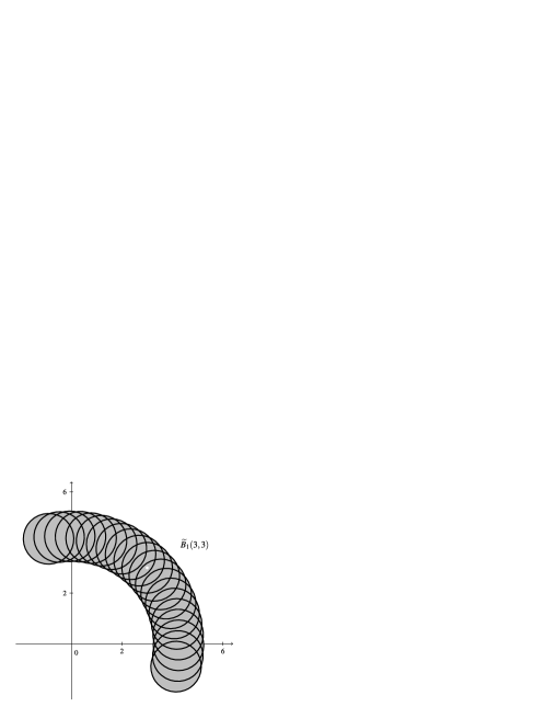
Figure 1: The quasi-ball $\tilde{B}$ of radius $1$ and center $(3,3)$.

We introduce a linear operator by setting

$$(Tf)(x)=\int_{0}^{\infty}(\Delta E_{t})\ast(f\circ O_{t})(x)\,\mathrm{d}t,$$

where $\Delta=\partial_{1}^{2}+\partial_{2}^{2}$, $f\in\mathscr{S}(\mathbb{R}^{2})$ and $(f\ast g)(x)=\int_{\mathbb{R}^{2}}f(y)g(x-y)\,\mathrm{d}y$. Setting $\psi=\Delta E$ and $\psi_{r}=\frac{1}{r}\psi\circ D_{r^{-1}}$, we obtain

$$(Tf)(x)=\int_{0}^{\infty}\psi_{t}\ast(f\circ O_{t})(x)\,\frac{\mathrm{d}t}{t},\quad f\in\mathscr{S},\ x\in\mathbb{R}^{2}.$$ (1)

Note that $\int\psi_{r}(x)\,\mathrm{d}x=0$, which implies some cancellation when smooth functions are convoluted with $\psi_{t}$ and $t$ is small. This cancellations suffices to make the integral in (1) converge. The arguments used in [4] suggest that $T$ can be extended to a bounded linear operator on $\mathrm{L}^{p}$ if $1<p<\infty$. The operator $T$ is said to be of weak type (1,1) or bounded from $\mathrm{L}^{1}$ to $\mathrm{L}^{1,\infty}$, if ${\mu}\left(\left\{x\ :\ \left\lvert Tf(x)\right\rvert>\lambda\right\}\right)\leq C\frac{\left\lVert f\right\rVert_{1}}{\lambda}$ for all $\lambda>0$ and all $f$. So far, we had no hints on whether $T$ is of weak type (1,1). We will show that this is indeed the case. The proof will rely on quasi-balls $\tilde{B}$ as the one depicted in Figure 1. More precisely, we define the quasi-balls $\tilde{B}_{r}$ as unions of Euclidean balls of radius $r^{\frac{1}{2}}$ by

$$\tilde{B}_{r}(z)=\bigcup_{-r\leq s\leq r}\left\{x\in\mathbb{R}^{2}\ :\ \left\lVert x\right\rVert_{2}<r^{\frac{1}{2}}\right\}+O_{s}(z),\quad z\in\mathbb{R}^{2},r>0.$$

An example where $G$ is nonabelian. The set $\mathbb{C}^{2}\times\mathbb{R}$ together with the product

$$[(u_{1},v_{1},s_{1}),(u_{2},v_{2},s_{2})]=(0,0,\operatorname{Im}(\overline{u_{1}}u_{2}+\overline{v_{1}}v_{2}))$$

is a real Lie algebra. Furthermore, the product

$$x\cdot y=x+y+\frac{1}{2}[x,y],\quad x,\,y\in\mathbb{C}^{2}\times\mathbb{R}$$

defines a real Lie group, the Heisenberg group $\mathbb{H}_{2}$. If $\alpha,\beta\in\mathbb{R}$, the symplectic automorphisms $O_{t}(u,v,s)=(ue^{i\alpha t},ve^{i\beta t},s)$ can be viewed as rotations and the automorphisms $D_{t}(u,v,s)=(tu,tv,t^{2}s)$ as nonisotropic dilations, yielding a noncommutative example for the general case.

The more general setting presented below has been described and explained by Folland and Stein [6, Chap. 1]. We add the notion of rotations. For the sake of simplicity, the assumptions are slightly redundant.

Assumptions

Let $G$ be a connected and simply connected nilpotent Lie group with Lie algebra $\mathfrak{g}$, $\dim\mathfrak{g}=n\geq 2$. We identify $G$ with $\mathfrak{g}$ via the group exponential function, so $G$ is the manifold $\mathfrak{g}$ together with a group product that is given by the Campbell-Hausdorff formula and the Lie product $[\cdot,\cdot]$ on $\mathfrak{g}$. In this setting the neutral element of $G$ equals $0_{\mathfrak{g}}$. We have the identities $x^{-1}=-x$, $xy=x+y+\frac{1}{2}[x,y]+\ldots$, $\exp_{G}=\operatorname{Id}$ and $\operatorname{Aut}G=\operatorname{Aut}\mathfrak{g}\subseteq\mathrm{GL}(\mathfrak{g})$.

We assume that $A$ is a diagonalizable linear operator on $\mathfrak{g}$ whose eigenvalues are positive and that $\{\exp(A\log t)\}_{t}$ is a family of Lie algebra automorphisms. Furthermore, we assume that $\{D_{t}\}_{t>0}$ is a family of Lie group automorphisms such that $dD_{t}(e)=\exp(A\log t)$. Then $\{D_{t}\}_{t>0}$ is called a family of dilations and $G$ is called a homogeneous group with respect to $\{D_{t}\}_{t}$. $Q=\operatorname{trace}A$ is called its homogeneous dimension. The maps $D_{t}=\exp(A\log t)$ are linear.

Let $O:\mathbb{R}\to\operatorname{Aut}(G)$ be a continuous homomorphism whose image is relatively compact. We also write $\{O_{t}\}_{t\in\mathbb{R}}$ instead of $O$ and refer to $\{O_{t}\}_{t\in\mathbb{R}}$ as the family of rotations. We assume that rotations commute with dilations, which amounts to saying that the eigenspaces of nontrivial dilations are left invariant by rotations.

From now on we identify $\mathfrak{g}$ (and hence $G$) with $\mathbb{R}^{n}$. The map $t\mapsto\operatorname{det}O_{t}$ is a continuous homomorphism from $(\mathbb{R},+)$ to $(\mathbb{R}\setminus\{0\},\cdot)$. Since $\operatorname{det}{O_{\mathbb{R}}}$ is a subset of the compact set $\operatorname{det}({\overline{O_{\mathbb{R}}}})$ in $\mathbb{R}$, it is also bounded. Hence for every $t$ we have $\operatorname{det}O_{t}=1$ and $O_{t}\in\mathrm{SL}(n)$. Since the closure of $\left\{O_{t}\ :\ t\in\mathbb{R}\right\}$ is a compact Lie subgroup of the connected group $\mathrm{SL}(n)$, it can be conjugated into the maximal compact subgroup $\mathrm{SO}(n)$ of $\mathrm{SL}(n)$ [8]. Therefore, the identification of $\mathfrak{g}$ with $\mathbb{R}^{n}$ can be done in such a way that $O_{t}\in\mathrm{SO}(n)$ for all $t$, and we will proceed on this assumption. We define $\mathscr{S}(G)$ to be $\mathscr{S}(\mathbb{R}^{n})$ and use the Euclidean Schwartz norms

$$\left\lVert f\right\rVert_{(N)}=\sup_{\left\lvert\alpha\right\rvert\leq N,\ x\in G}\left<x\right>^{N}\left\lvert\partial^{\alpha}f(x)\right\rvert,\quad\left<x\right>=\left(1+\left\lVert x\right\rVert_{2}^{2}\right)^{\frac{1}{2}},\ x\in\mathbb{R}^{n}.$$

Instead, Schwartz norms defined in terms of invariant vector fields and a homogeneous norm could be used, see [6, p. 35].

We use the Lebesgue measure $\mathrm{d}x$ on $G$ and denote it by $\mu$ when measuring sets, that is, $\mu(M)=\int_{M}\mathrm{d}x$. This is a left- and right-invariant Haar measure. Let $\mathrm{L}^{p}$ and $\mathrm{L}^{1,\infty}$ be the Lorentz spaces $\mathrm{L}^{p}(G,\mathrm{d}x)$ and $\mathrm{L}^{1,\infty}(G,\mathrm{d}x)$ respectively. Note that $\left\lVert\,\cdot\,\right\rVert_{1,\infty}$ is a quasinorm, and that $\mathrm{L}^{1,\infty}$ is complete [7, Thm. 1.4.11.]. We denote the convolution of $f$ and $g$ by $(f\ast g)(x)=\int_{G}f(xy^{-1})g(y)\,\mathrm{d}y$. For any function $\psi:G\to\mathbb{C}$ and $t>0$ we denote by $\psi_{t}=t^{-Q}\psi\circ D_{t^{-1}}$ the $\mathrm{L}^{1}$-invariantly dilated function $\psi_{t}$.

The singular integral operator

We fix some $\psi\in\mathscr{S}(G)$ with $\int\psi(x)\,\mathrm{d}x=0$ and define

$$(Tf)(x)=\int_{0}^{\infty}[\psi_{t}\ast(f\circ O_{t})](x)\,\frac{\mathrm{d}t}{t},\quad f\in\mathscr{S},\ x\in G.$$ (2)

With techniques similar to the ones used in the proof of Lemma 3, it can be shown that (2) converges. For the proof of the following theorem, we will rely on a definition of $T$ as an operator on $\mathrm{L}^{2}(G)$, which is compatible with (2).

Theorem 1.

Let $1<p\leq 2$ and $T$ as in (2). There exists a constant $C$ such that for all $f\in\mathscr{S}$ and all $\lambda>0$ we have the estimates

$${\mu}\left(\left\{x\in G\ :\ \left\lvert Tf(x)\right\rvert>\lambda\right\}\right)\leq C\frac{\left\lVert f\right\rVert_{1}}{\lambda}$$ (3)

and

$$\left\lVert Tf\right\rVert_{p}\leq C\left\lVert f\right\rVert_{p}.$$ (4)

Hence $T$ has a unique extension to a bounded linear operator on $\mathrm{L}^{p}$, $p\in]1,2]$ and a unique extension to a bounded linear operator from $\mathrm{L}^{1}$ to $\mathrm{L}^{1,\infty}$. On the premise that $\psi(O_{t}x)=\psi(x)$ for all $t$ and $x$, the preceding is also true for $2<p<\infty$.

2 Prerequisites

Homogeneous norms.  A continuous function $\left\lvert\cdot\right\rvert:G\to[0,\infty)$ is said to be a homogeneous norm on $G$ with respect to $\{D_{t}\}_{t}$ if it satisfies $\left\lvert x\right\rvert=0\ \Leftrightarrow\ x=0$,  $\left\lvert x^{-1}\right\rvert=\left\lvert x\right\rvert$ and  $\left\lvert D_{t}x\right\rvert=t\left\lvert x\right\rvert$ for all $t>0$ and $x\in G$. Some authors require homogeneous norms to be smooth away from the origin. There exists a homogeneous norm $\left\lvert\cdot\right\rvert$ that is invariant under rotations; that is,

$$\left\lvert O_{t}x\right\rvert=\left\lvert x\right\rvert$$ (5)

for all $x$, $t$. For a hint on how to produce such homogeneous norms, see the example in Sect. 7. We will keep one such homogeneous norm fixed. The terms $\left\lvert x^{-1}y\right\rvert$ and $\left\lvert xy^{-1}\right\rvert$ define left-invariant and right-invariant quasi-distance functions respectively. These quasi-distances are symmetric and coincide if $G$ is abelian. We refer to them as the homogeneous distance between $x$ and $y$. We use the term quasi-metric for symmetric quasi-distance functions; namely, if $d$ is a quasi-metric then $x=y\ \Leftrightarrow\ d(x,y)=0$,  $d(x,y)=d(y,x)$, and there is a constant $\kappa$ such that  $d(x,y)\leq\kappa(d(x,z)+d(z,y))$.

Balls and spheres.   Balls and spheres with center $0$ and with respect to $\left\lvert\cdot\right\rvert$ are defined by $B_{r}=\left\{x\in G\ :\ \left\lvert x\right\rvert<r\right\}$ and $S_{r}=\left\{x\in G\ :\ \left\lvert x\right\rvert=r\right\}$ respectively. The ball with center $z$ and with respect to the left- and right-invariant quasi-metrics are equal to $z\cdot B_{r}$ and $B_{r}\cdot z$ respectively.

Integration.   The definition of $Q$ is natural in the sense that there exists a constant $C$ so that $\int_{B_{r}\cdot z}\,\mathrm{d}x=Cr^{Q},\ \text{for all }z\in G,\ r>0$ and that $\det D_{r}=r^{Q}$. Furthermore, there exists a positive Borel measure $\sigma$ on $S_{1}$ such that all $f\in\mathrm{L}^{1}(G)$ can be integrated using spherical coordinates by

$$\int_{G}f(x)\,dx=\int_{0}^{\infty}\int_{S_{1}}f(D_{r}x)\,\mathrm{d}\sigma(x)r^{Q-1}\,\mathrm{d}r.$$ (6)

Since $O_{t}\in\mathrm{SL}(n)$, $\mu$ is invariant under rotations:

$$\int f(x)\,\mathrm{d}x=\int(f\circ O_{t})(x)\,\mathrm{d}x$$ (7)

for every $f$ and $t$. Note that $f_{r}\ast g_{r}=(f\ast g)_{r}$, and that $(f\ast g)\circ O_{t}=(f\circ O_{t})\ast(g\circ O_{t})$, for all $f,g\in\mathrm{L}^{1}(G)$, $t\in\mathbb{R}$, $s>0$.

Constants.   We will use miscellaneous constants $C,C^{\prime},C_{1}>0$ etc. whose values vary from line to line and who may depend on the geometric setting, for example, on the homogeneous group. Occasionally we write $a(x)\lesssim b(x)$ or $a\lesssim b$ to indicate that there is a constant $C$ such that $a(x)\leq C\cdot b(x)$ for all $x$. Furthermore, $a\simeq b$ shall mean that for some $C_{1},C_{2}$, we have $a(x)\leq C_{1}\cdot b(x)\leq C_{2}\cdot a(x)$ for all $x$.

Norm estimates.   By $\gamma$ we denote the smallest eigenvalue of $A$ and by $\Gamma$ the greatest eigenvalue of $A$.

For any vector space norm $\left\lVert\cdot\right\rVert$ and any relatively compact neighborhood $U$ of the origin there exist constants $C_{1},C_{2}>0$ such that we have the norm estimate

$$\left\lvert x\right\rvert^{\Gamma}\leq C_{1}\left\lVert x\right\rVert\leq C_{2}\left\lvert x\right\rvert^{\gamma}\quad\text{for all }x\in U$$ (8)

and

$$\left\lvert x\right\rvert^{\gamma}\leq C_{1}\left\lVert x\right\rVert\leq C_{2}\left\lvert x\right\rvert^{\Gamma}\quad\text{for all }x\in G\setminus U.$$ (9)

Cancellation.   The quantity $\left\lvert\psi(x)-\psi(y)\right\rvert$ can be estimated in various ways in terms of the distance between $x$ and $y$, for example, see [6, p. 28]. The following lemma is fine for our purpose.

Lemma 2.

For any $l\in\mathbb{N}$ there exists a constant $C$ and a Schwartz norm $\left\lVert\cdot\right\rVert_{(N)}$ such that for all $\psi\in\mathscr{S}(G)$ and all $x,y\in G$ we have

$$\left\lvert\psi(x)-\psi(y)\right\rvert\leq C\left\lVert\psi\right\rVert_{(N)}\cdot\left\lvert x^{-1}y\right\rvert^{\gamma}\cdot\left(\frac{1}{(1+\left\lVert x\right\rVert_{2})^{l}}+\frac{1}{(1+\left\lVert y\right\rVert_{2})^{l}}\right).$$

Proof.

We find $N$ and $C$ such that the Lemma is true on the additional assumption that $\left\lvert x^{-1}y\right\rvert\geq 1$, because $\psi\in\mathscr{S}$. We will possibly increase the values of $N$ and $C$ later. Now let $\left\lvert x^{-1}y\right\rvert\leq 1$. Since the map

$$h:G\times G\to G,\quad(x,z)\mapsto x-xz$$

is smooth, any derivative of $h$ is bounded on any compact set. Furthermore, we have $h(x,0)=0$. Now compactness and the norm estimate (8) yield for any $x$ with $\left\lvert x\right\rvert\leq 1$

$$\left\lVert x-y\right\rVert_{2}=\left\lVert h(x,x^{-1}y)\right\rVert_{2}\leq C_{1}\left\lVert x^{-1}y\right\rVert_{2}\leq C_{2}\left\lvert x^{-1}y\right\rvert^{\gamma}.$$ (10)

If $t=\left\lvert x\right\rvert\geq 1$, using (10) with $x-y$ replaced by $D_{t^{-1}}x-D_{t^{-1}}y$, we obtain

$$\begin{split}\left\lVert x-y\right\rVert_{2}&=\left\lVert D_{t}(D_{t^{-1}}x-D_{t^{-1}}y)\right\rVert_{2}\leq\left\lVert D_{t}\right\rVert_{\mathrm{op}}\left\lVert D_{t^{-1}}x-D_{t^{-1}}y\right\rVert_{2}\\ &\leq Ct^{\Gamma}\left\lvert(D_{t^{-1}}x)^{-1}(D_{t^{-1}}y)\right\rvert^{\gamma}=Ct^{\Gamma-\gamma}\left\lvert x^{-1}y\right\rvert^{\gamma}=C\left\lvert x\right\rvert^{\Gamma-\gamma}\left\lvert x^{-1}y\right\rvert^{\gamma}.\end{split}$$ (11)

Interchanging the roles of $x$ and $y$ in (11) and combining with (10), we get

$$\left\lVert x-y\right\rVert_{2}\leq C(1+\min\{\left\lvert x\right\rvert,\left\lvert y\right\rvert\}^{\Gamma-\gamma})\left\lvert x^{-1}y\right\rvert^{\gamma}.$$

With the help of (9) we find some $p\in\mathbb{N}$ such that $\left\lvert z\right\rvert^{\Gamma-\gamma}\leq C\left\lVert z\right\rVert_{2}^{p}$ for all $z\in G\setminus B_{1}$. Setting $R=\min\{\left\lVert x\right\rVert_{2},\left\lVert y\right\rVert_{2}\}$, it follows that

$$\left\lVert x-y\right\rVert_{2}\leq C(1+R)^{p}\left\lvert x^{-1}y\right\rvert^{\gamma}.$$ (12)

We choose an integration path from $x$ to $y$ in $M=\left\{z\in G\ :\ \left\lVert z\right\rVert_{2}\geq R\right\}$ such that the length of this path is bounded by a constant multiple of $\left\lVert x-y\right\rVert_{2}$. Let us estimate $\left\lvert\psi(x)-\psi(y)\right\rvert$ by integrating along that path. Since $\psi\in\mathscr{S}$, we find a number $N$ such that

$$\left\lVert(\nabla\psi)(1+\left\lVert\cdot\right\rVert_{2})^{l+p}\right\rVert_{\infty}\leq\left\lVert\psi\right\rVert_{(N)}.$$ (13)

Putting (12) and (13) together, we obtain

$$\left\lvert\psi(x)-\psi(y)\right\rvert\leq C_{1}\left\lVert(\nabla\psi)1_{M}\right\rVert_{\infty}\left\lVert x-y\right\rVert_{2}\leq C_{2}\frac{\left\lVert\psi\right\rVert_{(N)}}{(1+R)^{l+p}}(1+R)^{p}\left\lvert x^{-1}y\right\rvert^{\gamma}.$$

Finally, because of

$$\frac{1}{(1+R)^{l}}\leq\frac{1}{(1+\left\lVert x\right\rVert_{2})^{l}}+\frac{1}{(1+\left\lVert y\right\rVert_{2})^{l}},$$

we get the desired result. ∎

Lemma 3.

There is a constant $C$ and a Schwartz norm $\left\lVert\cdot\right\rVert_{(N)}$ such that for all $\varphi\in\mathscr{S}(G)$ with $\int\varphi=0$, all $\psi\in\mathscr{S}$, and all $0<s<1$ we have

$$\left\lVert\psi\ast\varphi_{s}\right\rVert_{1}\leq C\left\lVert\psi\right\rVert_{(N)}\left\lVert\varphi\right\rVert_{(N)}s^{\gamma}\quad\text{and}\quad\left\lVert\psi_{s}\ast\varphi\right\rVert_{1}\leq C\left\lVert\psi\right\rVert_{(N)}\left\lVert\varphi\right\rVert_{(N)}s^{\gamma}.$$

Proof.

We give a proof of the first inequality. Using Lemma 2 with $l=n+1$, we obtain

$$\begin{split}\left\lVert\psi\ast\varphi_{s}\right\rVert_{1}&=\int\left\lvert\int\psi(xy^{-1})\varphi_{s}(y)\,dy\right\rvert\,dx\\ &=\int\left\lvert\int[\psi(xy^{-1})-\psi(x)]\varphi_{s}(y)\,dy\right\rvert\,dx\\ &=\int\int\left\lvert\psi(xy^{-1})-\psi(x)\right\rvert\cdot\left\lvert\varphi_{s}(y)\right\rvert\,dy\,dx\\ &\leq C\left\lVert\psi\right\rVert_{(N)}\int\int\left\lvert y\right\rvert^{\gamma}(\frac{1}{(1+\left\lVert x\right\rVert_{2})^{n+1}}+\frac{1}{(1+\left\lVert xy^{-1}\right\rVert_{2})^{n+1}})\left\lvert\varphi_{s}(y)\right\rvert\,dy\,dx\\ &\leq C\left\lVert\psi\right\rVert_{(N)}\int\left\lvert y\right\rvert^{\gamma}\int(\frac{1}{(1+\left\lVert x\right\rVert_{2})^{n+1}}+\frac{1}{(1+\left\lVert xy^{-1}\right\rVert_{2})^{n+1}})\,dx\left\lvert\varphi_{s}(y)\right\rvert\,dy\\ &\leq C\left\lVert\psi\right\rVert_{(N)}\left(\int\frac{1}{(1+\left\lVert x\right\rVert_{2})^{n+1}}\,dx\right)\int\left\lvert y\right\rvert^{\gamma}\left\lvert\varphi_{s}(y)\right\rvert\,dy\\ &\leq C\left\lVert\psi\right\rVert_{(N)}\int\left\lvert D_{s}y\right\rvert^{\gamma}\varphi(y)\,dy\\ &\leq C\left\lVert\psi\right\rVert_{(N)}s^{\gamma}\int\left\lvert y\right\rvert^{\gamma}\varphi(y)\,dy\\ &\leq C\left\lVert\psi\right\rVert_{(N)}\left\lVert\varphi\right\rVert_{(N)}s^{\gamma}.\end{split}$$

∎

3 $\mathrm{L}^{2}$ results

The space $\mathrm{L}^{2}(G)$ together with the product $\langle f|g\rangle=\int_{G}f(x)\overline{g(x)}\,\mathrm{d}x$ is a Hilbert space. This allows to extend the linear operator $T$ defined by (2) to a bounded operator on $\mathrm{L}^{2}(G)$, yielding (4) for $p=2$. Observe that the operators

$$A_{t}:\mathrm{L}^{2}(G)\to\mathrm{L}^{2}(G),\quad A_{t}f=\psi_{t}\ast(f\circ O_{t}),\quad t>0.$$

are bounded by Young’s inequality, which is valid in the context of homogeneous groups, and by (7). Namely, we have $\left\lVert A_{t}\right\rVert\leq\left\lVert\psi\right\rVert_{1}$ for every $t>0$; and $A_{t}^{\ast}f=(\psi_{t}^{\ast}\ast f)\circ O_{-t}$, where $\psi_{t}^{\ast}(x)=\overline{\psi(x^{-1})}$.
The set $\mathcal{E}=\left\{E\subseteq]0,\infty[\ :\ E\text{ measurable and }\int_{E}\,\frac{\mathrm{d}t}{t}<\infty\right\}$ ordered by inclusion is a directed set.

Theorem 4.

The net $\left(\int_{E}A_{t}\,\frac{\mathrm{d}t}{t}\right)_{E\in\mathcal{E}}$ converges in the weak operator topology to a bounded linear operator $\widetilde{T}$ on $\mathrm{L}^{2}(G)$, whose restriction to $\mathscr{S}$ equals $T$.

Proof.

The main task is to show that there is a function $h$ such that

$$\left\lVert A_{t}A_{s}^{\ast}\right\rVert^{\scriptstyle\frac{1}{2}}\leq h(t,s)\quad\text{ and }\quad\left\lVert A_{t}^{\ast}A_{s}\right\rVert^{\scriptstyle\frac{1}{2}}\leq h(t,s)$$ (14)

and

$$\sup_{s>0}\int_{0}^{\infty}h(t,s)\,\frac{\mathrm{d}t}{t}\ <\infty.$$ (15)

Then the proof will be finished by using a continuous version of Cotlar’s lemma [5, Appendix B]. Let $s,t>0$ and $f\in\mathrm{L}^{2}(G)$. We have the estimates

$$\begin{split}\left\lVert A_{t}A^{\ast}_{s}f\right\rVert_{2}&=\left\lVert\psi_{t}\ast[(\psi^{\ast}_{s}\ast f)\circ O_{s}^{-1}\circ O_{t}]\right\rVert_{2}\\ &=\left\lVert(\psi_{t}\circ O_{s-t})\ast(\psi^{\ast}_{s}\ast f)\right\rVert_{2}\\ &=\left\lVert[(\psi\circ O_{s-t})_{t}\ast\psi^{\ast}_{s}]\ast f)\right\rVert_{2}\\ &\leq\left\lVert(\psi\circ O_{s-t})_{t}\ast\psi^{\ast}_{s}\right\rVert_{1}\left\lVert f\right\rVert_{2},\end{split}$$

$$\begin{split}\left\lVert A_{t}^{\ast}A_{s}f\right\rVert_{2}&=\left\lVert(\psi^{\ast}_{t}\ast[\psi_{s}\ast(f\circ O_{s})])\circ O_{t}^{-1}\right\rVert_{2}\\ &\leq\left\lVert\psi_{t}^{\ast}\ast\psi_{s}\right\rVert_{1}\left\lVert f\right\rVert_{2}.\end{split}$$

Setting

$$h(t,s)=\left\lVert(\psi\circ O_{s-t})_{t}\ast\psi^{\ast}_{s}\right\rVert_{1}^{\scriptstyle\frac{1}{2}}+\left\lVert\psi_{t}^{\ast}\ast\psi_{s}\right\rVert_{1}^{\scriptstyle\frac{1}{2}},$$

we obtain (14). It remains to show (15). This can be done by using the Schwartz norms of $\psi\circ O_{s-t}$, which are bounded uniformly in $s$ and $t$, and Lemma 3. Let us consider an arbitrary family $\{\varphi^{s,t}\}_{s,t>0}$ of Schwartz functions such that $\left\lVert\varphi^{s,t}\right\rVert_{(N)}\leq C_{N}$ for all $s,t>0$. Furthermore, assume $\chi\in\mathscr{S}$ and $\int\varphi^{s,t}=\int\chi=0$ for all $s,t>0$. Then there exists a Schwartz norm $\left\lVert\cdot\right\rVert_{(N)}$ such that for all $s>0$ the estimate

$$\begin{split}\int_{0}^{\infty}\left\lVert\varphi^{s,t}_{t}\ast\chi_{s}\right\rVert_{1}^{\scriptstyle\frac{1}{2}}\,\frac{\mathrm{d}t}{t}&=\int_{0}^{\infty}\left\lVert\varphi^{s,ts}_{ts}\ast\chi_{s}\right\rVert_{1}^{\scriptstyle\frac{1}{2}}\,\frac{\mathrm{d}t}{t}\\ &=\int_{0}^{\infty}\left\lVert(\varphi^{s,ts}_{t}\ast\chi)_{s}\right\rVert_{1}^{\scriptstyle\frac{1}{2}}\,\frac{\mathrm{d}t}{t}\\ &=\int_{0}^{\infty}\left\lVert\varphi^{s,ts}_{t}\ast\chi\right\rVert_{1}^{\scriptstyle\frac{1}{2}}\,\frac{\mathrm{d}t}{t}\\ &=\int_{0}^{1}\left\lVert\varphi^{s,ts}_{t}\ast\chi\right\rVert_{1}^{\scriptstyle\frac{1}{2}}\,\frac{\mathrm{d}t}{t}+\int_{0}^{1}\left\lVert\varphi^{s,t^{-1}s}_{t^{-1}}\ast\chi\right\rVert_{1}^{\scriptstyle\frac{1}{2}}\,\frac{\mathrm{d}t}{t}\\ &=\int_{0}^{1}\left\lVert\varphi^{s,ts}_{t}\ast\chi\right\rVert_{1}^{\scriptstyle\frac{1}{2}}\,\frac{\mathrm{d}t}{t}+\int_{0}^{1}\left\lVert\varphi^{s,t^{-1}s}\ast\chi_{t}\right\rVert_{1}^{\scriptstyle\frac{1}{2}}\,\frac{\mathrm{d}t}{t}\\ &\leq C\left(\sup_{s,t}\left\lVert\varphi^{s,t}\right\rVert^{\scriptstyle\frac{1}{2}}_{(N)}\right)\left\lVert\chi\right\rVert^{\scriptstyle\frac{1}{2}}_{(N)}\int_{0}^{1}t^{\frac{\gamma}{2}}\,\frac{\mathrm{d}t}{t}\\ &\leq C\left(\sup_{s,t}\left\lVert\varphi^{s,t}\right\rVert^{\scriptstyle\frac{1}{2}}_{(N)}\right)\left\lVert\chi\right\rVert^{\scriptstyle\frac{1}{2}}_{(N)}\end{split}$$

holds. Setting $\varphi^{s,t}=\psi\circ O_{s-t}$, $\chi=\psi^{\ast}$; and $\varphi^{s,t}=\psi^{\ast}$, $\chi=\psi$; yields (15). It follows that $\widetilde{T}=\lim_{E\in\mathcal{E}}\int_{E}A_{t}\,\frac{\mathrm{d}t}{t}$ for some bounded operator $\widetilde{T}$ on $\mathrm{L}^{2}(G)$.

Let $f$ and $g$ be Schwartz functions. We have $\left\lVert A_{t}f\right\rVert_{\infty}\leq\left\lVert\psi_{t}\right\rVert_{\infty}\left\lVert f\right\rVert_{1}\leq Ct^{-Q}$ and furthermore, for $0<t<1$, Lemma 3 yields $\left\lVert A_{t}f\right\rVert_{1}\leq Ct^{\gamma}\left\lVert\psi\right\rVert_{(N)}\left\lVert f\right\rVert_{(N)}$. This results in

$$\int_{0}^{1}\int_{G}\left\lvert t^{-1}A_{t}(x)\cdot\overline{g(x)}\right\rvert\,\mathrm{d}x\,\mathrm{d}t<\int_{0}^{1}t^{-1}\left\lVert A_{t}f\right\rVert_{1}\cdot\left\lVert g\right\rVert_{\infty}\,\mathrm{d}t<\infty,$$

$$\int_{1}^{\infty}\int_{G}\left\lvert t^{-1}A_{t}(x)\cdot\overline{g(x)}\right\rvert\,\mathrm{d}x\,\mathrm{d}t<\int_{1}^{\infty}t^{-1}\left\lVert A_{t}f\right\rVert_{\infty}\cdot\left\lVert g\right\rVert_{1}\,\mathrm{d}t<\infty,$$

that is, $(t,x)\mapsto\left\lvert t^{-1}A_{t}(x)\cdot\overline{g(x)}\right\rvert$ is integrable. Fubini’s Theorem yields

$$\begin{split}&\langle\widetilde{T}f|g\rangle\\ &=\lim_{E}\int_{E}\langle A_{t}f|g\rangle\,\frac{\mathrm{d}t}{t}\\ &=\int_{0}^{\infty}\int_{G}t^{-1}A_{t}(x)\cdot\overline{g(x)}\,\mathrm{d}x\,\mathrm{d}t\\ &=\int_{G}\int_{0}^{\infty}t^{-1}A_{t}(x)\,\mathrm{d}t\cdot\overline{g(x)}\,\mathrm{d}x\\ &=\langle Tf|g\rangle,\end{split}$$ (16)

showing $\left.\widetilde{T}\right|_{\mathscr{S}}=T$. ∎

From now on we denote $\widetilde{T}$ by $T$ .

4 A space of homogeneous type

We now define quasi-balls $\tilde{B}\subseteq G$. For any $r>0$ and $y\in G$ we set

$$\tilde{B}_{r}(y)=\bigcup_{s\in[-r,r]}B_{r}\cdot(O_{s}y).$$

Then by (5) we have $x\in\tilde{B}_{r}(y)\ \Leftrightarrow\ y\in\tilde{B}_{r}(x)\ \Leftrightarrow\ \exists s:\left\lvert s\right\rvert\leq r\wedge\left\lvert x\cdot O_{s}y^{-1}\right\rvert<r$ and $O_{s}(\tilde{B}_{r}(y))=\tilde{B}_{r}(O_{s}y)$. We show that the balls $\tilde{B}$ possess the engulfing and doubling properties as described by Stein in [10, p. 8].

Theorem 5.

There exist constants $C,k>0$ such that for all $x,y\in G$ and $t>0$

$$\tilde{B}_{t}(y)\cap\tilde{B}_{t}(x)\neq\emptyset\Rightarrow\tilde{B}_{t}(y)\subseteq\tilde{B}_{kt}(x),$$ (17)

$${\mu}(\tilde{B}_{2t}(x))\leq C\cdot{\mu}(\tilde{B}_{t}(x)).$$ (18)

Proof.

Choose $a_{1},\ldots,a_{l}\in G$ such that $B_{2}\subseteq\bigcup_{k=1}^{l}a_{k}B_{1}$. These exist, since $B_{2}$ is relatively compact and $\{z\cdot B_{1}\}_{z\in G}$ is an open covering of $\overline{B_{2}}$. It follows that $B_{2t}=D_{t}B_{2}\subseteq D_{t}(\bigcup_{k=1}^{l}a_{k}B_{1})\subseteq\bigcup_{k=1}^{l}(D_{t}a_{k})(D_{t}B_{1})=\bigcup_{k=1}^{l}(D_{t}a_{k})B_{t}$. Finally we obtain

$$\begin{split}{\mu}(\tilde{B}_{2t}(x))&={\mu}(B_{2t}\cdot\left\{O_{s}x\ :\ s\in[-2t,2t]\right\})\\ &\leq{\mu}\left(\left(\bigcup_{k=1}^{l}(D_{t}a_{k})\cdot B_{t}\right)\cdot\left(\bigcup_{\sigma=\pm t}\left\{O_{s+\sigma}x\ :\ \left\lvert s\right\rvert\leq t\right\}\right)\right)\\ &\leq{\mu}\left(\bigcup_{k=1}^{l}\bigcup_{\sigma=\pm t}(D_{t}a_{k})\cdot B_{t}\cdot\left\{O_{s+\sigma}x\ :\ \left\lvert s\right\rvert\leq t\right\}\right)\\ &\leq\sum_{k=1}^{l}\sum_{\sigma=\pm t}{\mu}\left(\ (D_{t}a_{k})\cdot B_{t}\cdot\left\{O_{s+\sigma}x\ :\ \left\lvert s\right\rvert\leq t\right\}\ \right)\\ &\leq\sum_{k=1}^{l}\sum_{\sigma=\pm t}{\mu}\left(\ O_{-\sigma}(B_{t}\cdot\left\{O_{s+\sigma}x\ :\ \left\lvert s\right\rvert\leq t\right\})\ \right)\\ &\leq\sum_{k=1}^{l}\sum_{\sigma=\pm t}{\mu}(\ B_{t}\cdot\left\{O_{s}x\ :\ \left\lvert s\right\rvert\leq t\right\}\ )\\ &=2l{\mu}(\tilde{B}_{t}(x)).\end{split}$$

This is the doubling property (18). The engulfing property (17) is known to be true when the quasi-balls $\tilde{B}_{t}$ are replaced by the simpler quasi-balls $B_{t}$. So we may choose a constant $k\geq 3$ such that (17) holds with $B_{t}$ instead of $\tilde{B}$, and proceed to prove (17).

Now assume that $\tilde{B}_{t}(x)\cap\tilde{B}_{t}(y)\neq\emptyset$. Choose $a,b\in[-t,t]$ such that $B_{t}\cdot(O_{a}x)\cap B_{t}\cdot(O_{b}y)\neq\emptyset$. Property (17) with $B$ instead of $\tilde{B}$ yields $B_{t}(O_{a}x)\subseteq B_{kt}(O_{b}y)$. Let $s\in[-t,t]$. Rotating both sets with $O_{s-a}$ and keeping in mind that $\left\lvert s-a+b\right\rvert\leq 3t\leq kt$, we conclude that $B_{t}\cdot(O_{s}x)\subseteq B_{kt}(O_{s-a+b}y)\subseteq\tilde{B}_{kt}(y)$, that is, $\tilde{B}_{t}(x)\subseteq\tilde{B}_{kt}(y)$. ∎

Corollary 6.

The Hardy-Littlewood maximal operator

$$(Mf)(x)=\sup_{r>0}\frac{1}{{\mu}({\tilde{B}_{r}(x))}}\int_{\tilde{B}_{r}(x)}\left\lvert f(y)\right\rvert\,dy$$

is of weak type (1,1).

For a proof, see [10] for example. The quasi-balls $\tilde{B}$ define a quasi-metric

$$d(x,y)=\inf\left\{r>0\ :\ x\in\tilde{B}_{r}(y)\right\}.$$ (19)

This quasi-metric yields a space of homogeneous type in the sense of Coifman and Weiss [2]. Note that for any quasi-metric there are constants $C_{1},C_{2},C_{3}\geq 1$ such that for all $x,y,\bar{y}$ we have

$$C_{1}\cdot d(y,\bar{y})<d(x,y)\Rightarrow d(x,y)\leq C_{2}d(x,\bar{y})\leq C_{3}d(x,y).$$ (20)

5 The integral kernel

In this section we study singular integral kernels $K(x,y)$ related to $T$. Let $\eta:G\to\mathbb{C}$ be a continuous function such that $\left\lVert\eta\right\rVert_{\infty}=C_{1}<\infty$ and $\sup_{x}\left\lvert\eta(x)\left\lvert x\right\rvert^{N}\right\rvert=C_{2}<\infty$ for some $N>Q$.

Lemma 7.

The integral

$$K_{\eta}(x,y)=\int_{0}^{\infty}\eta_{t}(x\cdot O_{-t}y^{-1})\,\frac{\mathrm{d}t}{t},\quad x\neq y,\ x,y\in G$$ (21)

converges and defines a continuous function $K:G\times G\setminus\left\{(x,x)\ :\ x\in G\right\}\to\mathbb{C}$. There exists a constant $C$ such that

$$\left\lvert K_{\eta}(x,y)\right\rvert\leq C\cdot[d(x,y)]^{-Q}$$ (22)

for all $x,y\in G$, $x\neq y$. The estimate (22) remains true if in (21) $O_{-t}$ is replaced by $O_{t}$ or $x\cdot O_{-t}y^{-1}$ by $(O_{-t}x)\cdot y^{-1}$.

Proof.

Assume that $x_{0},y_{0}\in G$ and that $d(x_{0},y_{0})=\epsilon>0$. Then for any $0\leq t\leq\epsilon$ we have

$$\left\lvert x_{0}\cdot O_{-t}y_{0}^{-1}\right\rvert\geq\epsilon$$

and there is a $\delta>0$ such that

$$\left\lvert x\cdot O_{-t}y^{-1}\right\rvert\geq\frac{\epsilon}{2}\quad\text{for all}\ x\in B_{\delta}\cdot x_{0},\ y\in B_{\delta}\cdot y_{0}\ \text{ and }\ 0\leq t\leq\epsilon.$$ (23)

We will construct a function $H:\mathbb{R}^{+}\to\mathbb{R}^{+}$ such that

$$\left\lvert\eta_{t}(x\cdot O_{-t}y^{-1})\right\rvert\leq H(t)\quad\text{for all}\ x\in B_{\delta}\cdot x_{0},\ \;y\in B_{\delta}\cdot y_{0}\ \text{ and }\ 0\leq t\leq\epsilon$$ (24)

and such that

$$\int_{0}^{\infty}H(t)\,\frac{\mathrm{d}t}{t}\leq C\epsilon^{-Q},$$ (25)

where $C$ is a constant depending on $\eta$, but not on $x$ or $y$. Then the estimate (22) is obvious. Furthermore, the convergence of the integral and the continuity of $K$ follow by the dominated convergence theorem. To prove (25), note that $\eta_{t}(x\cdot O_{-t}y^{-1})=t^{-Q}\eta\circ h(t)$, where $h(t)=D_{t^{-1}}(x\cdot O_{-t}y^{-1})$. Because of (23), $\left\lvert h\right\rvert$ is bounded from below by $\left\lvert h(t)\right\rvert=t^{-1}\left\lvert x\cdot O_{-t}y^{-1}\right\rvert\geq{\scriptstyle\frac{1}{2}}t^{-1}\epsilon\geq{\scriptstyle\frac{1}{2}}$ for $0\leq t\leq\epsilon$, and $\eta$ is bounded from above by

$$\left\lvert\eta\circ h(t)\right\rvert\leq\frac{C_{2}}{\left\lvert h(t)\right\rvert^{N}}\leq C_{2}2^{N}\cdot t^{N}\cdot\epsilon^{-N}.$$ (26)

Then $H(t)=t^{-Q}\begin{cases}C_{1}&t>\epsilon\\ C_{2}2^{N}t^{N}\epsilon^{-N}&t\leq\epsilon\end{cases}$ yields (24) and (25), which finishes the proof of Lemma 7. ∎

For example, $\eta=\psi$ and $\eta=\left\lvert\psi\right\rvert$ satisfy the assumptions of Lemma 7. Note that (22) is weaker than the condition

$$\left\lvert K(x,y)\right\rvert\leq\frac{C}{{\mu}(\tilde{B}_{d(x,y)}(y))}$$

required for standard Calderón-Zygmund kernels, see Sect. 8.

The pointwise estimate (22) does not suggest integrability of $K(\cdot,y)$:

$$\int_{G}[d(x,y)]^{-Q}\,\mathrm{d}x\geq\int_{G}\left\lvert xy^{-1}\right\rvert^{-Q}\,\mathrm{d}x=C\int_{0}^{\infty}r^{-Q}r^{Q-1}\,\mathrm{d}r=\infty.$$

Nonetheless, if $K_{\eta}=\,^{\epsilon}\!K_{\eta}+K^{\epsilon}_{\eta}$, where

$$^{\epsilon}\!K_{\eta}(x,y)=\int_{0}^{\epsilon}\eta_{t}(x\cdot O_{-t}y^{-1})\,\frac{\mathrm{d}t}{t},\quad x\neq y,\ x,y\in G,$$ (27)

$$K^{\epsilon}_{\eta}(x,y)=\int_{\epsilon}^{\infty}\eta_{t}(x\cdot O_{-t}y^{-1})\,\frac{\mathrm{d}t}{t},\quad x,y\in G,$$ (28)

then ${}^{\epsilon}\!K_{\eta}(\,\cdot\,,y_{0})$ is a function that is integrable at infinity and $K^{\epsilon}_{\eta}$ is a bounded function such that for every $y_{0}$ the kernel satisfies some estimate $K^{\epsilon}_{\eta}(x,y_{0})\lesssim\left\lvert x\right\rvert^{-Q}$ as $x$ tends to infinity. If $\eta\geq 0$ and $\eta(0)>0$, then even $K^{\epsilon}_{\eta}(x,y_{0})\gtrsim\left\lvert x\right\rvert^{-Q}$ .

Lemma 8.

There is a constant $C$ such that for all $y$, $\eta$, and $\epsilon$, we have

$$\int_{d(x,y)>\epsilon}\left\lvert\,{}^{\epsilon}\!K_{\eta}(x,y)\right\rvert\,\mathrm{d}x\leq C\cdot\sup_{x}\left\lvert\eta(x)\left\lvert x\right\rvert^{N}\right\rvert.$$

Proof.

Without loss of generality we assume $\eta\geq 0$ and $C_{2}$ as before. Assume that $0<\epsilon\leq d(x,y)$ and $0<t<\epsilon$. Then we have $\left\lvert x\cdot O_{-t}y^{-1}\right\rvert\geq\epsilon$. Substituting $z$ for $x\cdot O_{-t}y^{-1}$, we obtain $\left\lvert z\right\rvert\geq\epsilon$ and, using spherical coordinates (6), we obtain the estimate

$$\begin{split}&\int_{d(x,y)>\epsilon}\int_{0}^{\epsilon}\eta_{t}(x\cdot O_{-t}y^{-1})\,\frac{\mathrm{d}t}{t}\,\mathrm{d}x\\ &\leq\int_{0}^{\epsilon}\int_{\left\lvert z\right\rvert\geq\epsilon}\eta_{t}(z)\,\mathrm{d}z\,\frac{\mathrm{d}t}{t}\\ &\leq\int_{0}^{\epsilon}\int_{\left\lvert z\right\rvert\geq\frac{\epsilon}{t}}\eta(z)\,\mathrm{d}z\,\frac{\mathrm{d}t}{t}\\ &\leq\sigma(S_{1})\int_{0}^{\epsilon}\int_{\frac{\epsilon}{t}}^{\infty}\frac{C_{2}}{r^{N}}r^{Q-1}\,\mathrm{d}r\,\frac{\mathrm{d}t}{t}\\ &\leq C\cdot C_{2}\int_{0}^{\epsilon}\left(\frac{\epsilon}{t}\right)^{Q-N}\,\frac{\mathrm{d}t}{t}\ \\ &\leq C\cdot C_{2}.\end{split}$$

∎

Lemma 9.

The operator $T$ is expressible as a singular integral as follows. For all $f\in\mathrm{L}^{2}(G)$ with compact support and all $x\in G\setminus\operatorname{supp}f$, the integrals

$$Tf(x)=\int_{G}K_{\psi}(x,y)f(y)\,\mathrm{d}y\quad\text{and}\quad T^{\ast}f(x)=\int_{G}\overline{K_{\psi}(y,x)}f(y)\,\mathrm{d}y$$

converge and equality holds for almost all $x\in G\setminus\operatorname{supp}f$.

Proof.

The function $K_{\left\lvert\psi\right\rvert}$ is continuous by Lemma 7. If $f,g\in\mathrm{L}^{2}(G)$ have compact support and $\operatorname{supp}f\cap\operatorname{supp}g=\emptyset$, then we have the estimate

$$\begin{split}\infty>&\int_{G}\int_{G}K_{\left\lvert\psi\right\rvert}(x,y)\left\lvert f(y)\right\rvert\left\lvert g(x)\right\rvert\,\mathrm{d}y\,\mathrm{d}x\\ &=\int_{G}\int_{G}\int_{0}^{\infty}\left\lvert\psi_{t}(x\cdot O_{-t}y^{-1})\cdot f(y)\cdot\overline{g(x)}\right\rvert\,\frac{\mathrm{d}t}{t}\,\mathrm{d}x\,\mathrm{d}y.\end{split}$$

Tonelli’s and Fubini’s Theorems imply that

$$\begin{split}&\int_{G}\int_{G}K_{\psi}(x,y)f(y)\,dy\ \overline{g(x)}\,dx\\ &=\int_{G}\int_{G}\int_{0}^{\infty}\psi_{t}(x\cdot O_{-t}y^{-1})\cdot f(y)\cdot\overline{g(x)}\,\frac{\mathrm{d}t}{t}\,\mathrm{d}x\,\mathrm{d}y\\ &=\int_{0}^{\infty}\int_{G}\int_{G}\psi_{t}(x\cdot O_{-t}y^{-1})\cdot f(y)\,\mathrm{d}y\ \overline{g(x)}\,\mathrm{d}x\,\frac{\mathrm{d}t}{t}\\ &=\int_{0}^{\infty}\int_{G}\int_{G}\psi_{t}(x\cdot y^{-1})\cdot f(O_{t}y)\,\mathrm{d}y\ \overline{g(x)}\,\mathrm{d}x\,\frac{\mathrm{d}t}{t}\\ &=\int_{0}^{\infty}\langle\psi_{t}\ast(f\circ O_{t})|g\rangle\,\frac{\mathrm{d}t}{t}\\ &=\int_{0}^{\infty}\langle A_{t}f|g\rangle\,\frac{\mathrm{d}t}{t}\\ &=\langle Tf|g\rangle,\end{split}$$

where $O_{t}y$ has been substituted for $y$. A similar calculation yields

$$\int_{G}\int_{G}\overline{K_{\psi}(y,x)}f(y)\,\mathrm{d}y\ \overline{g(x)}\,\mathrm{d}x=\langle T^{\ast}f|g\rangle.$$

Finally, let $\overline{B}\subseteq G$ be a compact ball with rational radius and rational center such that $\overline{B}\subseteq G\setminus\operatorname{supp}f$. Then $\int_{G}K_{\psi}(x,y)f(y)\,dy$ converges for all $x\in\overline{B}$,

$$\langle Tf|g\rangle=\langle\int_{G}K_{\psi}(\,\cdot\,,y)f(y)\,\mathrm{d}y|g\rangle$$

holds for all $g\in\mathrm{L}^{2}(B)$ and hence $Tf(x)=\int_{G}K_{\psi}(x,y)f(y)\,\mathrm{d}y$ for almost all $x\in\overline{B}$. Since there are only countably many balls $\overline{B}$ and every $x\in G\setminus\operatorname{supp}f$ is contained in such a ball, we have equality for almost all $x\in G\setminus\operatorname{supp}f$.

Similar arguments apply to $T^{\ast}$. ∎

We will need the following technical lemma.

Lemma 10.

There is a constant $C_{1}>0$ such that, for all $x\in G$, $t>0$ and $s\in[-\frac{t}{2},\frac{t}{2}]$,

$$\left\lvert(D_{t-s}^{-1}x)^{-1}(D_{t}^{-1}x)\right\rvert\leq C_{1}\left\lvert D_{t}^{-1}x\right\rvert\cdot\left(\frac{\left\lvert s\right\rvert}{t}\right)^{\frac{1}{\Gamma}}.$$

Proof.

The map

$$h:\left\{x\in G\ :\ \left\lvert x\right\rvert=1\right\}\times[-\frac{1}{3},2]\to G,\quad(x,p)\mapsto x^{-1}D_{1+p}x$$

is the restriction of a smooth map to a compact set. Since furthermore $h(x,0)=0$, we find a constant $C$ such that for all $p\in[-\frac{1}{3},2]$ we have

$$\left\lvert x\right\rvert=1\Rightarrow\left\lVert x^{-1}D_{1+p}x\right\rVert_{2}\leq C\left\lvert p\right\rvert.$$

The norm estimate (8) yields

$$\left\lvert x\right\rvert=1\Rightarrow\left\lvert x^{-1}D_{1+p}x\right\rvert\leq C\left\lvert p\right\rvert^{\frac{1}{\Gamma}}.$$

Setting $p=\frac{t}{t-s}-1=\frac{s}{t-s}$, we obtain the estimate

$$\left\lvert x\right\rvert=1\ \Rightarrow\ \left\lvert x^{-1}D_{\frac{t}{t-s}}x\right\rvert\leq C\left\lvert\frac{s}{t-s}\right\rvert^{\frac{1}{\Gamma}}\leq C_{1}\left\lvert\frac{s}{t}\right\rvert^{\frac{1}{\Gamma}},$$

and for arbitrary $x$ with $\left\lvert x\right\rvert=r$, we have

$$C_{1}\left\lvert\frac{s}{t}\right\rvert^{\frac{1}{\Gamma}}\geq\left\lvert(D_{r}^{-1}x^{-1})D_{\frac{t}{t-s}}D_{r}^{-1}x\right\rvert=r^{-1}t\left\lvert(D_{t}^{-1}x^{-1})(D_{t-s}^{-1}x)\right\rvert.$$

Finally, multiplying with $r\cdot t^{-1}$ yields

$$C_{1}\left\lvert\frac{s}{t}\right\rvert^{\frac{1}{\Gamma}}t^{-1}\left\lvert x\right\rvert\geq\left\lvert(D_{t}^{-1}x^{-1})(D_{t-s}^{-1}x)\right\rvert=\left\lvert(D_{t-s}^{-1}x)^{-1}(D_{t}^{-1}x)\right\rvert.$$

∎

Theorem 11.

There are constants $k$ and $C$ and a Schwartz norm $\left\lVert\cdot\right\rVert_{(N)}$ such that for all $\psi\in\mathscr{S}(G)$, $\delta>0$, $y\in G$, $\bar{y}\in\tilde{B}_{\delta}(y)$ it holds that

$$\int_{G\setminus\tilde{B}_{k\delta}(y)}\left\lvert K_{\psi}(x,y)-K_{\psi}(x,\bar{y})\right\rvert\,\mathrm{d}x\leq\ C\left\lVert\psi\right\rVert_{(N)}.$$ (29)

If in addition $\psi(O_{t}x)=\psi(x)$ for all $t$ and $x$, then

$$\int_{G\setminus\tilde{B}_{k\delta}(y)}\left\lvert\overline{K_{\psi}(y,x)}-\overline{K_{\psi}(\bar{y},x)}\right\rvert\,\mathrm{d}x\leq\ C\left\lVert\psi\right\rVert_{(N)}.$$ (30)

Proof.

Given the assumption about $\psi$, we have

$$\overline{K(y,x)}=\int_{0}^{\infty}\psi^{\ast}_{t}(x\cdot O_{t}y^{-1})\,\frac{\mathrm{d}t}{t}.$$

Therefore, (30) can be proven like (29) with minor changes. We prove (29): Because of (20), there is some $k\geq 3$ such that $d(x,y)\geq k\delta\wedge d(y,\bar{y})<\delta\Rightarrow d(x,\bar{y})\geq 2\delta$ for every $\delta>0$. Let $\delta>0$ and $y,\bar{y}\in G$ such that $d(y,\bar{y})<\delta$. Let $s$ be a number such that $\left\lvert O_{s}y\bar{y}^{-1}\right\rvert<\delta$ and $\left\lvert s\right\rvert\leq\delta$. Lemma 8 yields the estimate

$$\int_{d(x,y)>k\delta}\left\lvert\,{}^{2\delta-s}\!K_{\psi}(x,y)-\,^{2\delta}\!K_{\psi}(x,\bar{y})\right\rvert\leq C\left\lVert\psi\right\rVert_{(N_{0})},$$ (31)

for some Schwartz norm $\left\lVert\,\cdot\,\right\rVert_{(N_{0})}$. Hence, it is sufficient to show that

$$\int_{G}\left\lvert K^{2\delta-s}_{\psi}(x,y)-K^{2\delta}_{\psi}(x,\bar{y})\right\rvert\,\mathrm{d}x\leq C\left\lVert\psi\right\rVert_{(N^{\prime})}.$$ (32)

Observe that by substituting $t-s$ for $t$, we have

$$K^{2\delta-s}_{\psi}(x,y)=\int_{2\delta-s}^{\infty}\psi_{t}(x\cdot O_{-t}y^{-1})\,\frac{\mathrm{d}t}{t}=\int_{2\delta}^{\infty}\frac{\psi_{t-s}(x\cdot O_{-t+s}y^{-1})}{t-s}\,\mathrm{d}t.$$ (33)

This transformation yields additional cancellation because afterward, in (32), at the same value of $t$, the function $\psi$ is evaluated in two points of small homogeneous distance. To improve the estimates, we decompose the kernel integral in (32) further. Setting

$$a(t,x)=\frac{\psi_{t-s}(x\cdot O_{-t+s}y^{-1})}{t-s}\ \text{ and }\ d(t,x)=\frac{\psi_{t}(x\cdot O_{-t}\bar{y}^{-1})}{t},$$

$$b(t,x)=\frac{\psi_{t-s}(x\cdot O_{-t}\bar{y}^{-1})}{t-s}\ \text{ and }\ c(t,x)=\frac{\psi\circ D_{t-s}^{-1}(x\cdot O_{-t}\bar{y}^{-1})}{t^{Q+1}},$$

we have

$$\begin{split}&\left\lvert K^{2\delta-s}_{\psi}(x,y)-K^{2\delta}_{\psi}(x,\bar{y})\right\rvert\\ &\leq\int_{2\delta}^{\infty}\left\lvert a(t,x)-d(t,x)\right\rvert\,\mathrm{d}t\\ &=\int_{2\delta}^{\infty}\left\lvert a(t,x)-b(t,x)+b(t,x)-c(t,x)+c(t,x)-d(t,x)\right\rvert\,\mathrm{d}t\\ &\leq\int_{2\delta}^{\infty}\left\lvert a(t,x)-b(t,x)\right\rvert\,\mathrm{d}t+\int_{2\delta}^{\infty}\left\lvert b(t,x)-c(t,x)\right\rvert\,\mathrm{d}t+\int_{2\delta}^{\infty}\left\lvert c(t,x)-d(t,x)\right\rvert\,\mathrm{d}t.\end{split}$$ (34)

Note that in these integrals $t-s\simeq t$. The proof will be completed by showing that the estimate (32) holds with the integrand replaced by each of the three $t$-integrals at the end of (LABEL:split). The first of these integrals is

$$\begin{split}&\int_{G}\int_{2\delta}^{\infty}\left\lvert a(t,x)-b(t,x)\right\rvert\,\mathrm{d}t\,\mathrm{d}x\\ &\leq C\int_{2\delta}^{\infty}\int_{G}t^{-Q}\left\lvert\psi\circ D_{t-s}^{-1}(x\cdot O_{-t+s}y^{-1})-\psi\circ D_{t-s}^{-1}(x\cdot O_{-t}\bar{y}^{-1})\right\rvert\,\mathrm{d}x\,\frac{\mathrm{d}t}{t},\end{split}$$ (35)

which, by Lemma 2, is bounded by

$$\begin{split}&C\int_{2\delta}^{\infty}\int_{G}t^{-Q}\ C\left\lVert\psi\right\rVert_{(N_{1})}\left\lvert D_{t-s}^{-1}[(O_{s}y)\bar{y}^{-1}]\right\rvert^{\gamma}H(x,t)\ \mathrm{d}x\,\frac{\mathrm{d}t}{t},\end{split}$$ (36)

where

$$H(x,t)=\left(\frac{1}{(1+\left\lVert D_{t-s}^{-1}[x\cdot O_{-t+s}y^{-1}]\right\rVert_{2})^{l}}+\frac{1}{(1+\left\lVert D_{t-s}^{-1}[x\cdot O_{-t}\bar{y}^{-1}]\right\rVert_{2})^{l}}\right)$$

and $l>n$. Note that there is a $C$ such that for every $t$

$$\int_{G}H(x,t)\,\mathrm{d}x\leq Ct^{Q}.$$

Hence (36) continues as

$$\begin{split}&\int_{G}\int_{2\delta}^{\infty}\left\lvert a(t)-b(t)\right\rvert\,\mathrm{d}t\,\mathrm{d}x\\ &\leq C\left\lVert\psi\right\rVert_{(N_{1})}\int_{2\delta}^{\infty}t^{-Q}\,t^{Q}\,\left\lvert D_{t-s}^{-1}[(O_{s}y)\bar{y}^{-1}]\right\rvert^{\gamma}\,\frac{\mathrm{d}t}{t}\\ &\leq C\left\lVert\psi\right\rVert_{(N_{1})}\int_{2\delta}^{\infty}\ t^{-\gamma}\delta^{\gamma}\,\frac{\mathrm{d}t}{t}\\ &\leq C\left\lVert\psi\right\rVert_{(N_{1})}.\end{split}$$ (32ab)

The second integral can be written as

$$\begin{split}&\int_{G}\int_{2\delta}^{\infty}\left\lvert b(t,x)-c(t,x)\right\rvert\,\mathrm{d}t\,\mathrm{d}x\\ &=\int_{G}\int_{2\delta}^{\infty}\left\lvert\frac{\psi_{t-s}(x\cdot O_{-t}\bar{y}^{-1})}{t-s}-\frac{\psi\circ D_{t-s}^{-1}(x\cdot O_{-t}\bar{y}^{-1})}{t^{Q+1}}\right\rvert\\ &=\int_{2\delta}^{\infty}\int_{G}\left\lvert(t-s)^{-Q-1}-t^{-Q-1}\right\rvert\cdot\left\lvert\psi\circ D_{t-s}^{-1}(x\cdot O_{-t}\bar{y}^{-1})\right\rvert\,\mathrm{d}x\,\mathrm{d}t\\ &=\int_{2\delta}^{\infty}\left\lvert(t-s)^{-Q-1}-t^{-Q-1}\right\rvert\int_{G}\cdot\left\lvert\psi\circ D_{t-s}^{-1}(x)\right\rvert\,\mathrm{d}x\,\mathrm{d}t.\end{split}$$

This yields the estimate

$$\begin{split}&\int_{G}\int_{2\delta}^{\infty}\left\lvert b(t,x)-c(t,x)\right\rvert\,\mathrm{d}t\,\mathrm{d}x\\ &\leq C\int_{2\delta}^{\infty}t^{Q-2}\left\lvert s\right\rvert\int_{G}\cdot\left\lvert\psi\circ D_{t-s}^{-1}(x)\right\rvert\,\mathrm{d}x\,\mathrm{d}t\\ &\leq C\int_{2\delta}^{\infty}t^{Q-1}\delta\int_{G}\cdot\left\lvert\psi\circ D_{t-s}^{-1}(x)\right\rvert\,\mathrm{d}x\,\frac{\mathrm{d}t}{t}\\ &\leq C\int_{2\delta}^{\infty}t^{Q-1}\delta\ \cdot(t-s)^{Q}\left\lVert\psi\right\rVert_{1}\,\frac{\mathrm{d}t}{t}\\ &\leq C\left\lVert\psi\right\rVert_{1}\delta\int_{2\delta}^{\infty}t^{-1}\,\frac{\mathrm{d}t}{t}\\ &\leq C\left\lVert\psi\right\rVert_{1}\\ &\leq C\left\lVert\psi\right\rVert_{(N_{2})}.\end{split}$$ (32bc)

This was the second part. The third part is

$$\begin{split}&\int_{G}\int_{2\delta}^{\infty}\left\lvert c(t,x)-d(t,x)\right\rvert\,\mathrm{d}t\,\mathrm{d}x\\ &=\int_{G}\int_{2\delta}^{\infty}\left\lvert\frac{\psi\circ D_{t-s}^{-1}(x\cdot O_{-t}\bar{y}^{-1})}{t^{Q+1}}-\frac{\psi_{t}(x\cdot O_{-t}\bar{y}^{-1})}{t}\right\rvert\,\mathrm{d}t\,\mathrm{d}x\\ &=\int_{2\delta}^{\infty}\int_{G}t^{-Q}\left\lvert\psi\circ D_{t-s}^{-1}(x\cdot O_{-t}\bar{y}^{-1})-\psi\circ D_{t}^{-1}(x\cdot O_{-t}\bar{y}^{-1})\right\rvert\mathrm{d}x\,\frac{\mathrm{d}t}{t}\\ &=\int_{2\delta}^{\infty}\int_{G}t^{-Q}\left\lvert\psi(D_{t-s}^{-1}x)-\psi(D_{t}^{-1}x)\right\rvert\mathrm{d}x\,\frac{\mathrm{d}t}{t}\\ &\leq C\left\lVert\psi\right\rVert_{(N)}\int_{2\delta}^{\infty}\int_{G}t^{-Q}\left\lvert(D_{t-s}^{-1}x)^{-1}(D_{t}^{-1}x)\right\rvert^{\gamma}H(x,t)\mathrm{d}x\,\frac{\mathrm{d}t}{t}.\\ \end{split}$$ (37)

The last step relies on Lemma 2, where $l$ has been chosen such that $\int_{G}\left\lvert D_{t}^{-1}x\right\rvert^{\gamma}\cdot H(x,t)\,\mathrm{d}x<\infty$, and $H$ is the function

$$H(x,t)=\frac{1}{(1+\left\lVert D_{t-s}^{-1}x\right\rVert_{2})^{l}}+\frac{1}{(1+\left\lVert D_{t}^{-1}x)\right\rVert_{2})^{l}}.$$ (38)

Since $\left\lvert s\right\rvert\leq\delta$ and $t\geq 2\delta$, we have $\left\lVert D_{\frac{t}{t-s}}\right\rVert\leq C$ and $\left\lVert D_{\frac{t-s}{t}}\right\rVert\leq C$, that is, $\left\lVert D_{t}^{-1}x\right\rVert_{2}\simeq\left\lVert D_{t-s}^{-1}x\right\rVert_{2}$, and the two summands in (38) are bounded by a constant multiple of the second one. Furthermore,

$$\int_{G}\left\lvert D_{t}^{-1}x\right\rvert^{\gamma}\cdot H(x,t)\,\mathrm{d}x\leq Ct^{Q}.$$

Using Lemma 10, we continue estimate (LABEL:ugk1) with

$$\begin{split}&\int_{G}\int_{2\delta}^{\infty}\left\lvert c(t,x)-d(t,x)\right\rvert\,\mathrm{d}t\,\mathrm{d}x\\ &\leq C\left\lVert\psi\right\rVert_{(N_{3})}\int_{2\delta}^{\infty}\int_{G}t^{-Q}\left(C_{1}\left\lvert D_{t}^{-1}x\right\rvert\cdot\left(\frac{\left\lvert s\right\rvert}{t}\right)^{\frac{1}{\Gamma}}\right)^{\gamma}H(x,t)\mathrm{d}x\,\frac{\mathrm{d}t}{t}\\ &\leq C\left\lVert\psi\right\rVert_{(N_{3})}\int_{2\delta}^{\infty}t^{-Q-\frac{\gamma}{\Gamma}}\delta^{\frac{\gamma}{\Gamma}}\int_{G}\left\lvert D_{t}^{-1}x\right\rvert^{\gamma}H(x,t)\mathrm{d}x\,\frac{\mathrm{d}t}{t}\\ &\leq C\left\lVert\psi\right\rVert_{(N_{3})}\int_{2\delta}^{\infty}t^{-Q-\frac{\gamma}{\Gamma}}\delta^{\frac{\gamma}{\Gamma}}t^{Q}\,\frac{\mathrm{d}t}{t}\\ &\leq C\left\lVert\psi\right\rVert_{(N_{3})}\delta^{\frac{\gamma}{\Gamma}}\int_{2\delta}^{\infty}t^{-\frac{\gamma}{\Gamma}}\,\frac{\mathrm{d}t}{t}\\ &\leq C\left\lVert\psi\right\rVert_{(N_{3})}.\end{split}$$ (32cd)

Adding (32ab),(32bc),(32cd) finishes the proof of (32) with $N^{\prime}=\max\{N_{1},N_{2},N_{3}\}$. ∎

6 Proof of Theorem 1

Proof.

The weak type result (3) and the $\mathrm{L}^{p}$-result (4) for $1<p<2$ follow with the help of [10, Theorem 3, p. 19], which relies on a Calderón-Zygmund decomposition of $f$, here with respect to the quasi-balls $\tilde{B}$. The relevant premises have been verified in Theorems 4,  5, and 11.

If $2<p<\infty$,  let $q=\frac{p}{p-1}$ and $M=\left\{g\in\mathscr{S}(G)\ :\ \left\lVert g\right\rVert_{q}<1\right\}$. Note that $q<2$. With the same arguments as in the proof of boundedness for $T$, but replacing $\overline{K(y,x)}$ for $K(x,y)$, it can be shown that $\left\lVert T^{\ast}g\right\rVert_{q}\leq C\left\lVert g\right\rVert_{q}$.  It follows that

$$\left\lVert Tf\right\rVert_{p}=\sup_{g\in M}\langle Tf|g\rangle=\sup_{g\in M}\langle f|T^{\ast}g\rangle\leq\sup_{g\in M}\left\lVert f\right\rVert_{p}\left\lVert T^{\ast}g\right\rVert_{q}\leq C_{p}\left\lVert f\right\rVert_{p}$$

for any $f\in\mathrm{L}^{2}\cap\mathrm{L}^{p}(G)$. ∎

7 Example

Let $G_{1}$ be the real vector space $\mathbb{C}\times\mathbb{R}^{n-2}$. We denote its elements by

$$x=(u,x^{\prime}),\quad u\in\mathbb{C},\quad x^{\prime}=(x_{3},\ldots,x_{n})\in\mathbb{R}^{n-2}.$$

Let $a,a_{3},\ldots a_{n}>0$. We introduce a family of dilations with $Q=2a+\sum_{j=3}^{n}a_{j}$ by

$$D_{r}x=(r^{a}u,r^{a_{3}}x_{3},\ldots,r^{a_{n}}x_{n})$$

and a family of rotations by $O_{t}(u,x^{\prime})=(e^{it}u,x^{\prime})$. There are several ways to define homogeneous norms on $G_{1}$, each of which has its own advantages. It is known that on any homogeneous group any two homogeneous norms $\left\lvert\,\cdot\,\right\rvert$ and $\left\lvert\,\cdot\,\right\rvert^{\prime}$ are equivalent in the sense that $\left\lvert\,\cdot\,\right\rvert\simeq\left\lvert\,\cdot\,\right\rvert^{\prime}$. The volumes of the corresponding balls and quasi-balls are also equivalent in the sense that $\mu(\tilde{B}_{r}\cdot z)\simeq\mu(B_{r}^{\prime}\cdot z)$ and $\mu(\tilde{B}_{r}(z))\simeq\mu(\tilde{B}_{r}^{\prime}(z))$ if the balls $B,\tilde{B}$ and $B^{\prime},\tilde{B}^{\prime}$ are defined in terms of the homogeneous norms $\left\lvert\,\cdot\,\right\rvert$ and $\left\lvert\,\cdot\,\right\rvert^{\prime}$ respectively. Let us consider the homogeneous norms

$$\left\lvert x\right\rvert=\max\{\left\lvert u\right\rvert_{\mathbb{C}}^{\frac{1}{a}},\left\lvert x_{3}\right\rvert_{\mathbb{R}}^{\frac{1}{a_{3}}},\ldots,\left\lvert x_{n}\right\rvert_{\mathbb{R}}^{\frac{1}{a_{n}}}\},$$ (39)

$$\left\lvert x\right\rvert^{\prime}=\inf\left\{r>0\ :\ \left\lVert D_{r^{-1}}(x)\right\rVert_{2}<1\right\},$$

$$\left\lvert x\right\rvert^{\prime\prime}=\left(\left\lvert u\right\rvert_{\mathbb{C}}^{\frac{2}{a}}+\sum_{j=3}^{n}\left\lvert x_{j}\right\rvert^{\frac{2}{a_{j}}}\right)^{\frac{1}{2}}.$$

The second one has the advantage of being smooth away from the origin, while the first one allows effortless calculations. Throughout this section, we will use $\left\lvert\,\cdot\,\right\rvert$, and theorems will be valid for any homogeneous norm.

If $y=(v,y^{\prime})\in G_{1}$, and if we use the homogeneous norm given by (39), the quasi-metric (19) has the form

$$\begin{split}d(x,y)&=\inf\left\{r>0\ :\ \exists s:\left\lvert s\right\rvert\leq r\wedge\left\lvert x-O_{s}y\right\rvert<r\right\},\\ &=\min_{s\in\mathbb{R}}\max\left\{\left\lvert s\right\rvert,\,\left\lvert u-e^{is}v\right\rvert_{\mathbb{C}}^{\frac{1}{a}},\,\left\lvert x_{3}-y_{3}\right\rvert^{\frac{1}{a_{3}}},\,\left\lvert x_{n}-y_{n}\right\rvert^{\frac{1}{a_{n}}}\right\}.\end{split}$$

With $y$ and $r$ fixed, we have

$$\begin{split}&x\in\tilde{B}_{r}(y)\\ &\ \Leftrightarrow\ d(x,y)<r\\ &\ \Leftrightarrow\ \max\left\{\min_{\left\lvert s\right\rvert\leq r}\left\lvert u-e^{is}v\right\rvert_{\mathbb{C}}^{\frac{1}{a}},\,\left\lvert x_{3}-y_{3}\right\rvert_{\mathbb{R}}^{\frac{1}{a_{3}}},\,\left\lvert x_{n}-y_{n}\right\rvert_{\mathbb{R}}^{\frac{1}{a_{n}}}\right\}<r.\end{split}$$ (40)

Lemma 12.

For all $y=(v,y^{\prime})$ in $G_{1}$ and all $r>0$, the volume ${\mu}(\tilde{B}_{r}(y))$ is bounded from above and from below by a constant multiple of

$$r^{Q}+r^{Q-a}\left\lvert v\right\rvert\min\{1,r\}.$$

Proof.

As a first step, we consider the case $n=2$.

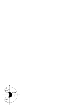
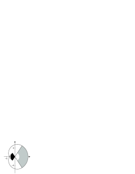
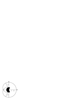
Figure 2: The sets $B^{\prime}(1,2,2)$,   $B^{\prime}(2,1,1)$ and  $B^{\prime}(2,2,1)$. The size of the black areas is $\pi(\left\lvert u\right\rvert-s)^{2}\frac{\min\{2\pi,\varphi\}}{2\pi}$, see equation (41).

For $v\in\mathbb{C}$, $\varphi\in\mathbb{R}$, and $r>0$ let

$$B^{\prime}(s,\varphi,v)=\bigcup_{\alpha\in[-\varphi,\varphi]}\left\{z\ :\ \left\lVert z\right\rVert_{2}<s\right\}+e^{i\alpha}v.$$

By some calculations corresponding to Fig. 2, we see that

$$\begin{split}{\mu}(B^{\prime}(s,\varphi,v))&\leq\pi s^{2}+\pi(\left\lvert v\right\rvert+s)^{2}\frac{\min\{2\pi,\varphi\}}{2\pi}-\pi(\left\lvert v\right\rvert-s)^{2}\frac{\min\{2\pi,\varphi\}}{2\pi}\\ &=\pi s^{2}+2s\cdot\left\lvert v\right\rvert\min\{2\pi,\varphi\}\\ &\leq 2{\mu}(B^{\prime}(s,\varphi,v)).\end{split}$$ (41)

Equality holds in the first two lines of (41) if $s<\left\lvert v\right\rvert$ and $\varphi<\frac{\pi}{2}$. Setting $s=r^{a}$ and $\varphi=r$, (41) yields

$${\mu}(\tilde{B}_{r}(y))={\mu}(B^{\prime}(r^{a},r,v))\simeq\pi r^{2a}+2r^{a}\cdot\left\lvert v\right\rvert\min\{2\pi,r\},$$ (42)

so we are done with the case $n=2$. Now let $n\geq 3$. Since

$$\tilde{B}_{r}(y)=B^{\prime}(r^{a},r,y)\times\prod_{j=3}^{n}(y_{j}-r^{a_{j}},y_{j}+r^{a_{j}})$$

we have

$$\begin{split}\mu(\tilde{B}_{r}(y))&=\mu(B^{\prime}(r^{a},r,y))\cdot(2r)^{Q-2a}\\ &\simeq\left(r^{2a}+r^{a}\cdot\left\lvert v\right\rvert\min\{1,r\}\right)r^{Q-2a},\end{split}$$

which completes the proof. ∎

The following Lemma roughly says that in $G_{1}$, the volume of the balls $\tilde{B}$ grows at least as in spaces of dimension $Q-a$.

Lemma 13.

There is a constant $C$ such that for any $y\in G_{1}$, $r\geq 0$ and $j\in\mathbb{N}$ we have

$${\mu}(\tilde{B}_{2^{j}r}(y))\geq C2^{j(Q-a)}{\mu}(\tilde{B}_{r}(y)).$$

Proof.

∎

Using Lemma 12 we obtain the estimate

$$\begin{split}{\mu}(\tilde{B}_{2^{j}r}(y))&\simeq(2^{j}r)^{Q}+(2^{j}r)^{Q-a}\left\lvert v\right\rvert\min\{1,2^{j}r\}\\ &=2^{j(Q-a)}\left(2^{ja}r^{Q}+r^{Q-a}\left\lvert v\right\rvert\min\{1,2^{j}r\}\right)\\ &\geq 2^{j(Q-a)}\left(r^{Q}+r^{Q-a}\left\lvert v\right\rvert\min\{1,r\}\right)\\ &\simeq C2^{j(Q-a)}{\mu}(\tilde{B}_{r}(y)).\end{split}$$ (43)

Lemma 14.

There is a constant $C_{1}$ such that for all $R\geq 1,\,r>0$ and $x,y\in G_{1}$ we have the estimate

$$\int_{r}^{2r}1_{\left\{t\ :\ \left\lvert x-O_{-t}y\right\rvert<Rt\right\}}\,\frac{\mathrm{d}t}{t}\leq C_{1}\frac{R^{a}r^{Q}}{{\mu}(\tilde{B}_{r}(y))}.$$ (44)

Furthermore, for any $p>a-Q$ there is a constant $C_{2}$ such that

$$\int_{r}^{\infty}t^{-Q-p}\cdot 1_{\left\{t\ :\ \left\lvert x-O_{-t}y\right\rvert<Rt\right\}}\,\frac{\mathrm{d}t}{t}\leq C_{2}\frac{R^{a}r^{-p}}{{\mu}(\tilde{B}_{r}(y))}$$ (45)

for all $r>0$ and all $x,y\in G_{1}$. These statements are also true when $O_{t}$ is substituted for $O_{-t}$ or when $x$ and $y$ are exchanged on one side.

Proof.

For some constants $C_{1},C_{2}$ we have ${\mu}(\tilde{B}_{r}(y))\leq C_{1}r^{Q}+C_{2}r^{Q-a}\left\lvert v\right\rvert\min\{1,r\}$ by Lemma 12. If ${\mu}(\tilde{B}_{r}(y))<2C_{1}r^{Q}$, then we are done with (44) because the left side of (44) is bounded by a constant. Otherwise we have ${\mu}(\tilde{B}_{r}(y))\geq 2C_{1}r^{Q}$ and

$${\mu}(\tilde{B}_{r}(y))\leq 2C_{2}r^{Q-a}\left\lvert v\right\rvert\min\{1,r\},$$

where $C_{2}$ does not depend on $y$ or $r$. Note that $v\neq 0$. Assume for the moment that

$$\int_{r}^{2r}1_{\left\{t\ :\ \left\lvert x-O_{-t}y\right\rvert<Rr\right\}}\ \mathrm{d}t\lesssim\frac{R^{a}r^{a+1}}{\left\lvert v\right\rvert\min\{r,1\}}.$$ (46)

Then, with $2R$ substituted for $R$, we get

$$\begin{split}\int_{r}^{2r}1_{\left\{t\ :\ \left\lvert x-O_{-t}y\right\rvert<Rt\right\}}\,\frac{\mathrm{d}t}{t}&\leq r^{-1}\int_{r}^{2r}1_{\left\{t\ :\ \left\lvert x-O_{-t}y\right\rvert<R2r\right\}}\ \mathrm{d}t\\ &\lesssim\frac{(2R)^{a}r^{Q}}{r^{Q-a}\left\lvert v\right\rvert\min\{r,1\}}\\ &\lesssim\frac{R^{a}r^{Q}}{{\mu}(\tilde{B}_{r}(y))},\end{split}$$

and the proof of (44) would be finished. So let us prove assumption (46). Note that by (39) we have

$$\left\lvert x-O_{-t}y\right\rvert<Rr\quad\Rightarrow\quad\left\lvert u-e^{-it}v\right\rvert^{\frac{1}{a}}_{\mathbb{C}}<Rr.$$

For any $0<r<r^{\prime}\leq r+2\pi$, it follows with the help of Fig. 3 that

$$\begin{split}\int_{r}^{r^{\prime}}1_{\left\{t\ :\ \left\lvert x-O_{-t}y\right\rvert<Rr\right\}}\ \mathrm{d}t&\leq{\mu}\left\{t\in[0,2\pi]\ :\ \ \left\lvert u-e^{-it}v\right\rvert<(Rr)^{a}\right\}\\ &={\mu}\left\{t\in[0,2\pi]\ :\ \ \left\lvert\frac{u}{\left\lvert v\right\rvert}-e^{-it}\frac{v}{\left\lvert v\right\rvert}\right\rvert<\frac{(Rr)^{a}}{\left\lvert v\right\rvert}\right\}\\ &\leq 2\pi\frac{(Rr)^{a}}{\left\lvert v\right\rvert}\\ &\lesssim\frac{R^{a}r^{a}}{\left\lvert v\right\rvert}.\\ \end{split}$$ (47)

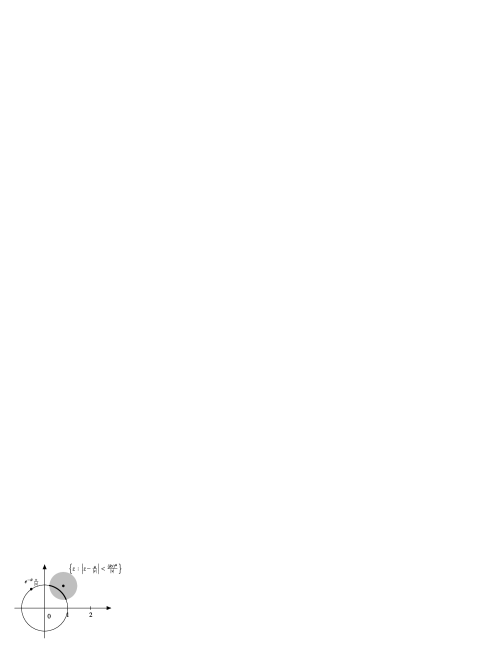
Figure 3: The length of the thick line is smaller than the circumference of the shaded area, see (47).

If $r<1$, then (46) follows from (47) with $r^{\prime}=2r$ because their right hand sides are equal. Otherwise, when $r\geq 1$, we decompose the integral into the sum

$$\begin{split}\int_{r}^{2r}1_{\left\{t\ :\ \left\lvert x-O_{-t}y\right\rvert<Rr\right\}}\ \mathrm{d}t&\leq\sum_{k=0}^{\lfloor r\rfloor}\int_{r+k}^{r+k+1}1_{\left\{t\ :\ \left\lvert x-O_{-t}y\right\rvert<Rr\right\}}\ \mathrm{d}t\\ &\lesssim\sum_{k=0}^{\lfloor r\rfloor}\frac{R^{a}\ (r+k)^{a}}{\left\lvert v\right\rvert}\\ &\lesssim\frac{R^{a}r^{a+1}}{\left\lvert v\right\rvert},\end{split}$$

which proves (46) and finishes the proof of (44). A dyadic decomposition of the interval $]0,\infty[$, equation (44) and Lemma 13 now yield

$$\begin{split}\int_{r}^{\infty}t^{-Q-p}\cdot 1_{\left\{t\ :\ \left\lvert x-O_{-t}y\right\rvert<Rt\right\}}\,\frac{\mathrm{d}t}{t}&=\sum_{j=0}^{\infty}\int_{2^{j}r}^{2^{j+1}r}t^{-Q-p}\cdot 1_{\left\{t\ :\ \left\lvert x-O_{-t}y\right\rvert<Rt\right\}}\,\frac{\mathrm{d}t}{t}\\ &\leq\sum_{j=0}^{\infty}(2^{j}r)^{-Q-p}\cdot C_{1}\cdot\frac{R^{a}(2^{j}r)^{Q}}{{\mu}(\tilde{B}_{2^{j}r}(y))}\\ &=C_{1}R^{a}r^{-p}\sum_{j=0}^{\infty}\frac{2^{-jp}}{{{\mu}(\tilde{B}_{2^{j}r}(y))}}\frac{{\mu}(\tilde{B}_{r}(y))}{{\mu}(\tilde{B}_{r}(y))}\\ &\lesssim\frac{R^{a}r^{-p}}{{\mu}(\tilde{B}_{r}(y))}\sum_{j=0}^{\infty}2^{-jp}\cdot 2^{j(a-Q)}\\ &\lesssim\frac{R^{a}r^{-p}}{{\mu}(\tilde{B}_{r}(y))},\end{split}$$

which proves (45). ∎

8 Calderón-Zygmund kernels

There is a number of related notions of ”standard” Calderón-Zygmund kernels in the context of homogeneous spaces, see [10, p. 29][3][9]. We say that $K$ is a Calderón-Zygmund kernel with respect to a quasi-metric $d$, corresponding quasi-balls $\tilde{B}$ and a measure ${\mu}$, if there exist constants $k>1$, $\epsilon>0$, and $C$ such that for all $x,y,\bar{y}$ the following estimates hold:

$$\left\lvert K(x,y)\right\rvert\leq\frac{C}{{\mu}(\tilde{B}_{d(x,y)}(y))}\quad\text{and}$$ (48)

$$\begin{split}\left\lvert K(y,x)-K(\bar{y},x)\right\rvert+\left\lvert K(x,y)-K(x,\bar{y})\right\rvert\\ \leq C\left(\frac{d(\bar{y},y)}{d(x,y)}\right)^{\epsilon}\cdot\frac{1}{{\mu}(\tilde{B}_{d(x,y)}(y))}\end{split}\qquad\text{ if }\ \ k\cdot d(y,\bar{y})<d(x,y).$$ (49)

There are hints that the kernels introduced in Sect. 5 are of this type. We examine an example in the setting made up in Sect. 7.

Theorem 15.

Let $G=G_{1}$, $D$, $d$, and $O$ as in Sect. 7 and let $K$ be a kernel $K_{\psi}$, where $\psi(O_{t}x)=\psi(x)$, $\operatorname{supp}\psi\subseteq B_{1}$ and $\int\psi=0$, as defined in Sect. 5. Then there exist $k$, $c$, $\epsilon$, and $C$ such that $K$ is a Calderón-Zygmund kernel in the sense of (48) and (49).

Proof.

We choose some $k\geq 4$ such that under the condition $k\cdot d(y,\bar{y})<d(x,y)$, we have $d(x,y)\simeq d(x,\bar{y})$ as in (20) and furthermore $4d(y,\bar{y})<d(x,\bar{y})$. Then it is sufficient to show (48) and (49) with $d(x,y)$ replaced by $\Delta=\min\{d(x,y),d(x,\bar{y})\}$. Note that if $x-O_{-t}y\in\operatorname{supp}\psi_{t}$ or $O_{t}x-y\in\operatorname{supp}\psi_{t}$, then $\left\lvert x-O_{-t}y\right\rvert<t$ and consequently $d(x,y)<t$. Thus we have

$$K(x,y)=\int_{\Delta}^{\infty}\psi_{t}(x-O_{-t}y)\,\frac{\mathrm{d}t}{t}$$

and Lemma 14 with $p=0$ yields

$$\begin{split}\left\lvert K(x,y)\right\rvert&\leq\left\lvert\int_{\Delta}^{\infty}t^{-Q}\left\lVert\psi\right\rVert_{\infty}\cdot 1_{\left\{t\ :\ \left\lvert x-O_{-t}y\right\rvert<t\right\}}\,\frac{\mathrm{d}t}{t}\right\rvert\\ &\leq C\left\lVert\psi\right\rVert_{\infty}\frac{1}{{\mu}(\tilde{B}_{\Delta}(y))},\end{split}$$

proving (48). We continue with the proof of (49), which is trivial if $y=\bar{y}$, so we assume $y\neq\bar{y}$. Due to the rotational symmetry of $\psi$, we have

$$K(\bar{y},x)=\int_{\Delta}^{\infty}\psi_{t}(O_{t}\bar{y}-x)\,\frac{\mathrm{d}t}{t}.$$ (50)

Setting $\delta=d(y,\bar{y})$, the estimate $0<4\delta<\Delta$ holds, and it suffices to verify that

$$\left\lvert K(x,y)-K(x,\bar{y})\right\rvert\leq C\left(\frac{\delta}{\Delta}\right)^{\epsilon}\cdot\frac{1}{{\mu}(\tilde{B}_{\Delta}(y))}$$ (51)

and

$$\left\lvert K(y,x)-K(\bar{y},x)\right\rvert\leq C\left(\frac{\delta}{\Delta}\right)^{\epsilon}\cdot\frac{1}{{\mu}(\tilde{B}_{\Delta}(y))}.$$ (52)

Because of (50), (52) can be shown with the same techniques as (51), so we prove (51) only. Choose some real number $s$, $\left\lvert s\right\rvert\leq\delta$, such that $\left\lvert O_{s}y-\bar{y}\right\rvert\leq\delta$. Then $\left\lvert s\right\rvert\leq\frac{1}{4}\Delta$ and

$$\begin{split}&\left\lvert K(x,y)-K(x,\bar{y})\right\rvert\\ &=\left\lvert\int_{\Delta}^{\infty}t^{-Q-1}\left[\psi(D_{t}^{-1}(x-O_{-t}y)-\psi(D_{t}^{-1}(x-O_{-t}\bar{y}))\right]\ \mathrm{d}t\right\rvert\\ &=\left\lvert\int_{\frac{3}{4}\Delta}^{\infty}\left[(t-s)^{-Q-1}\psi(D_{t-s}^{-1}(x-O_{-t+s}y))-t^{-Q-1}\psi(D_{t}^{-1}(x-O_{-t}\bar{y}))\right]\ \mathrm{d}t\right\rvert\\ &\leq\int_{\frac{3}{4}\Delta}^{\infty}(t-s)^{-Q-1}\cdot\left\lvert\psi(D_{t-s}^{-1}(x-O_{-t+s}y))-\psi(D_{t-s}^{-1}(x-O_{-t}\bar{y}))\right\rvert\ \mathrm{d}t\\ &\quad+\int_{\frac{3}{4}\Delta}^{\infty}\left\lvert(t-s)^{-Q-1}-t^{-Q-1}\right\rvert\cdot\left\lvert\psi(D_{t-s}^{-1}(x-O_{-t}\bar{y}))\right\rvert\ \mathrm{d}t\\ &\quad+\int_{\frac{3}{4}\Delta}^{\infty}t^{-Q-1}\cdot\left\lvert\psi(D_{t-s}^{-1}(x-O_{-t}\bar{y}))-\psi(D_{t}^{-1}(x-O_{-t}\bar{y})))\right\rvert\ \mathrm{d}t\\ &=\int_{\frac{3}{4}\Delta}^{\infty}f_{1}(t)\,\frac{\mathrm{d}t}{t}\ +\ \int_{\frac{3}{4}\Delta}^{\infty}f_{2}(t)\,\frac{\mathrm{d}t}{t}\ +\ \int_{\frac{3}{4}\Delta}^{\infty}f_{3}(t)\,\frac{\mathrm{d}t}{t},\end{split}$$

where $f_{1}$, $f_{2}$, and $f_{3}$ are the integrands in the preceding lines. They are supported in the sets

$$\begin{split}\operatorname{supp}f_{1}&\subseteq\left\{t>0\ :\ \left\lvert x-O_{-t}\bar{y}\right\rvert<2t\ \text{ or }\ \left\lvert x-O_{-t}(O_{s}y)\right\rvert<2t\right\},\\ \operatorname{supp}f_{2},\ \operatorname{supp}f_{3}&\subseteq\left\{t>0\ :\ \left\lvert x-O_{-t}\bar{y}\right\rvert<2t\right\}.\end{split}$$

Lemma 14 yields

$$\int_{\frac{3}{4}\Delta}^{\infty}t^{-Q-p}\cdot 1_{\{\operatorname{supp}f_{j}\}}\,\frac{\mathrm{d}t}{t}\ \lesssim\frac{\Delta^{-p}}{\mu(\tilde{B}_{\Delta}(x))}\lesssim\frac{\Delta^{-p}}{\mu(\tilde{B}_{\Delta}(y))},\quad j=1,2,3.$$ (53)

We now complete the proof by estimating the integrands $f_{j}$ against appropriate powers of $t$. We have

$$\begin{split}f_{1}(t)&=(t-s)^{-Q}\cdot\left\lvert\psi(D_{t-s}^{-1}(x-O_{-t+s}y))-\psi(D_{t-s}^{-1}(x-O_{-t}\bar{y}))\right\rvert\\ &\lesssim\left\lVert\nabla\psi\right\rVert_{\infty}t^{-Q}\left\lVert D_{t-s}^{-1}(O_{s}y-\bar{y})\right\rVert_{2}\\ &=\left\lVert\nabla\psi\right\rVert_{\infty}t^{-Q}\left\lVert D_{\frac{\delta}{t-s}}D_{\delta}^{-1}(O_{s}y-\bar{y})\right\rVert_{2}\\ &\leq\left\lVert\nabla\psi\right\rVert_{\infty}t^{-Q}\left\lVert D_{\frac{\delta}{t-s}}\right\rVert\\ &\leq C_{1}\left\lVert\nabla\psi\right\rVert_{\infty}\delta^{\gamma}t^{-Q-\gamma},\end{split}$$

where $\gamma=\min\{a,a_{2},\ldots,a_{n}\}$. Together with (53) this implies the inequality

$$\begin{split}&\int_{\frac{3}{4}\Delta}^{\infty}f_{1}(t)\,\frac{\mathrm{d}t}{t}\ \\ &\leq C_{1}\left\lVert\nabla\psi\right\rVert_{\infty}\delta^{\gamma}\int_{\frac{3}{4}\Delta}^{\infty}t^{-Q-\gamma}\cdot 1_{\{\operatorname{supp}f_{1}\}}\,\frac{\mathrm{d}t}{t}\\ &\leq C_{2}\left\lVert\nabla\psi\right\rVert_{\infty}\left(\frac{\delta}{\Delta}\right)^{\gamma}\frac{1}{\mu(\tilde{B}_{\Delta}(X))}.\end{split}$$ (54)

In a similar way we obtain

$$\begin{split}f_{2}(t)&=\left\lvert(t-s)^{-Q-1}-t^{-Q-1}\right\rvert\cdot\left\lvert\psi(D_{t-s}^{-1}(x-O_{-t}\bar{y}))\right\rvert t\\ &\leq C\left\lVert\psi\right\rVert_{\infty}\delta t^{-Q-1},\end{split}$$

$$\int_{\frac{3}{4}\Delta}^{\infty}f_{2}(t)\,\frac{\mathrm{d}t}{t}\ \leq\left\lVert\nabla\psi\right\rVert_{\infty}r\int_{\frac{3}{4}\Delta}^{\infty}t^{-Q-1}\cdot 1_{\{\operatorname{supp}f_{2}\}}\,\frac{\mathrm{d}t}{t}\ \leq\left\lVert\psi\right\rVert_{\infty}\frac{\delta}{\Delta}\cdot\frac{1}{{\mu}(\tilde{B}_{\Delta}(y))}.$$ (55)

Furthermore, we have the estimate

$$\begin{split}f_{3}(t)&=t^{-Q}\cdot\left\lvert\psi(D_{t-s}^{-1}(x-O_{-t}\bar{y}))-\psi(D_{t}^{-1}(x-O_{-t}\bar{y})\right\rvert\\ &\leq\left\lVert\nabla\psi\right\rVert_{\infty}t^{-Q}\cdot\left\lVert(D_{t-s}^{-1}-D_{t}^{-1})(x-O_{-t}\bar{y})\right\rVert_{2}\\ &=\left\lVert\nabla\psi\right\rVert_{\infty}\ t^{-Q}\cdot\left\lVert(D_{1-\frac{s}{t}}^{-1}-\operatorname{Id})D_{t}^{-1}(x-O_{-t}\bar{y})\right\rVert_{2}\\ &\leq\left\lVert\nabla\psi\right\rVert_{\infty}t^{-Q}\cdot\left\lVert(D_{1-\frac{s}{t}}^{-1}-\operatorname{Id})\right\rVert.\end{split}$$

Note that $p\mapsto D_{1-p}^{-1}-\operatorname{Id}$ is smooth, mapping $0$ to $0$, and that $\left\lvert\frac{s}{t}\right\rvert\leq\left\lvert\frac{\delta}{t}\right\rvert\leq\frac{1}{3}$. So we find a constant such that

$$f_{3}(t)\leq C\left\lVert\nabla\psi\right\rVert_{\infty}\delta t^{-Q-1},$$

and

$$\int_{\frac{3}{4}\Delta}^{\infty}f_{3}(t)\,\frac{\mathrm{d}t}{t}\ \leq\left\lVert\nabla\psi\right\rVert_{\infty}\delta\int_{\frac{3}{4}\Delta}^{\infty}t^{-Q-1}\cdot 1_{\{\operatorname{supp}f_{3}\}}\,\frac{\mathrm{d}t}{t}\ \leq\left\lVert\nabla\psi\right\rVert_{\infty}\frac{\delta}{\Delta}\cdot\frac{1}{{\mu}(\tilde{B}_{\Delta}(y))}.$$ (56)

Adding inequalities (LABEL:intf1) - (56) and using $\frac{\delta}{\Delta}\leq 1$, we obtain a constant C such that

$$\left\lvert K(x,y)-K(x,\bar{y})\right\rvert\leq C\cdot(\left\lVert\psi\right\rVert_{\infty}+\left\lVert\nabla\psi\right\rVert_{\infty})\left(\frac{\delta}{\Delta}\right)^{\min\{1,\gamma\ \}}\cdot\frac{1}{{\mu}(\tilde{B}_{\Delta}(y))}.$$

∎

Acknowledgments  This article evolved from my diploma thesis [1]. I would like to thank Prof. Müller (Kiel) and Prof. Ricci (Pisa) for their advice on the subject. The idea of choosing a homogeneous norm adapted to the family of rotations as in (5) is due to Prof. Ricci.

References

- [1] H. F. Bloch: Ein Integraloperator auf homogenen Gruppen. (unpublished)
- [2] R. R. Coifman, G. Weiss: Analyse Harmonique Non-Commutative sur Certains Espaces Homogenes. Lecture Notes in Mathematics, Vol. 242 (1971)
- [3] D. Deng, Y. Han and Y. Meyer: Harmonic Analysis on Spaces of Homogeneous Type. Lecture Notes in Mathematics, Springer (2009)
- [4] R. Farwig, T. Hishida, D. Müller: -Theory of a Singular “Winding” Integral Operator Arising from Fluid Dynamics. Pacific Journal of Mathematics, Vol. 215, p. 306 (2004)
- [5] G. B. Folland: Harmonic Analysis in Phase Space. Princeton University Press (1989)
- [6] G. B. Folland, E. M. Stein: Hardy Spaces on Homogeneous Groups. Princeton University Press (1982)
- [7] L. Grafakos: Classical Fourier Analysis, 2nd ed. Springer (2008)
- [8] J. Hilgert, K.-H. Neeb: Lie-Gruppen und Lie-Algebren, Vieweg, p. 277 (1991)
- [9] S. Hofmann: Weighted Norm Inequalities and Vector Valued Inequalities for Certain Rough Operators. Indiana University Mathematics Journal, Vol. 42, No.1, pp. 1-14 (1993)
- [10] E. M. Stein: Harmonic Analysis: Real-Variable Methods, Orthogonality and Oscillatory Integrals. Princeton University Press (1993)