Extracting generalized neutron parton distributions from ³He data

Abstract

An impulse approximation (IA) analysis is described of the generalized parton distributions (GPDs) $H$ and $E$ of the ³He nucleus, quantities which are accessible in hard exclusive processes, such as coherent deeply virtual Compton scattering (DVCS). The calculation is based on the Av18 interaction. The electromagnetic form factors are correctly recovered in the proper limits. The sum of the GPDs $H$ and $E$ of ³He, at low momentum transfer, is largely dominated by the neutron contribution, thanks to the unique spin structure of ³He. This nucleus is therefore very promising for the extraction of the neutron information. By increasing the momentum transfer, however, this conclusion is somehow hindered by the the fast growing proton contribution. Besides, even when the neutron contribution to the GPDs of ³He is largely dominating, the procedure of extracting the neutron GPDs from it could be, in principle, nontrivial. A technique is therefore proposed, independent on both the nuclear potential and the nucleon model used in the calculation, able to take into account the nuclear effects included in the IA analysis and to safely extract the neutron information at values of the momentum transfer large enough to allow the measurements. Thanks to this observation, coherent DVCS should be considered a key experiment to access the neutron GPDs and, in turn, the orbital angular momentum of the partons in the neutron.

I Introduction

Generalized Parton Distributions (GPDs) Mueller:1998fv ; Radyushkin:1996nd ; Ji:1996ek parametrize the non-perturbative hadron structure in hard exclusive processes, encoding therefore a wealth of information. For example, the hadron three-dimensional structure Burkardt:2000za and the parton total angular momentum could be unveiled by the measurement of GPDs, which will be therefore a major achievement for Hadronic Physics in the next few years. In particular, in order to access the hadron angular momentum content, from which the orbital angular momentum (OAM) part could be estimated by subtracting the helicity one, measurable in deep inelastic scattering inclusive (DIS) and semi-inclusive (SiDIS) processes, the knowledge of two GPDs is mandatory Ji:1996ek . They are the two chiral even, parton helicity independent GPDs occurring at leading twist, i.e., $H$, a target helicity-conserving quantity, and $E$, a target helicity-flip one. The cleanest experiment to access them is Deeply Virtual Compton Scattering (DVCS), i.e. the process $eH\longrightarrow e^{\prime}H^{\prime}\gamma$ when $Q^{2}\gg M^{2}$ (everywhere in this paper, $Q^{2}=-q\cdot q$ is the momentum transfer between the leptons $e$ and $e^{\prime}$, $\Delta^{2}$ the one between the hadrons $H$ and $H^{\prime}$ and $M$ is the nucleon mass) Ji:1996ek ; Vanderhaeghen:1999xj . Despite severe difficulties related to the complicated way GPDs enter the measured cross sections, DVCS data for proton and nuclear targets are being analyzed (recent results can be found in Refs. hermes ) and GPDs are being extracted (see Refs. Guidal:2010de and references therein).

The relevance of measuring GPDs for nuclear targets has been addressed in several papers, starting from Ref. cano1 , where the formalism for the deuteron target was presented. Soon after, DVCS off spin 0, $1/2$ and 1 nuclear targets has been detailed in Ref. kir_mue , and the impulse approximation (IA) approach to DVCS off spin 0 nuclei has been discussed in Ref. guzey1 . Microscopic calculations have been described for the GPDs of the deuteron in Ref. cano2 , and for spin zero nuclei in Ref. liuti1 ; a possible link of nuclear GPDs measurements to color transparency phenomena has been presented in Ref. liuti2 . One of the main motivations for addressing nuclear GPDs measurements is the possibility of distinguishing medium modifications of the structure of bound nucleons from conventional Fermi motion and binding effects, a cumbersome separation in data collected through standard DIS experiments. Off-shell effects have been studied in Ref. liuti3 and different medium modifications of nucleon GPDs have been illustrated in Ref. modif . The possibilities offered by heavy nuclear targets and the effects in nuclear matter are also being investigated nm .

The experimental study of nuclear GPDs could therefore seriously contribute to shed some light on the origin of the so called EMC effect emc , a puzzle still far to be solved. Great attention has anyway to be paid to avoid confusing unusual effects with conventional ones. To this respect, few-body nuclear targets, for which realistic studies are possible and exotic effects are in principle distinguishable, play a special role. To this aim, in Ref. io , an IA calculation of $H_{q}^{3}$, the GPD of ³He corresponding to the flavor $q$, has been presented, valid for $-\Delta^{2}\ll Q^{2},M^{2}$, and in particular, for $|\Delta^{2}|\lesssim 0.3$ GeV². The approach permits to investigate the coherent, no break-up channel of DVCS off ³He, whose cross-section, at $|\Delta^{2}|\simeq 0.3$ GeV², is already too small to be measured at present facilities. The main conclusion was that the nuclear GPDs cannot be trivially inferred from those of nuclear parton distributions (PDFs), measured in DIS.

In a recent Rapid Communication of ours, Ref. nostro , the approach of Ref. io has been extended to evaluate the GPD $E_{q}$ of ³He, $E_{q}^{3}$. The main goal was to study the possibility of accessing the neutron information, which is very relevant because it permits, together with the proton one, a flavor decomposition of GPDs data. One should not forget that the properties of the free neutron have to be investigated using nuclear targets, taking nuclear effects properly into account. In particular ³He, thanks to its peculiar spin structure, has the unique property of simulating an effective polarized free neutron target (see, e.g., friar ; antico ; SS ). ³He is therefore a serious candidate to measure the polarization properties of the free neutron, such as its helicity-flip GPD $E_{q}$. In Ref. nostro it has been found that the sum of the GPDs $H_{q}^{3}$ and $E_{q}^{3}$, at low momentum transfer, is indeed dominated to a large extent by the neutron contribution, making ³He targets very promising for the extraction of the neutron information. However, this is not the end of the story. The same analysis has shown in fact that the proton contribution grows fast with increasing the momentum transfer. Besides, even if the neutron contribution to the GPDs of ³He were largely dominating, the procedure of extracting the neutron GPDs from it could be, in principle, nontrivial. In this paper, a more comprehensive analysis is presented. In particular, a technique is proposed, independent on both the nuclear potential and the nucleon model used in the calculation, able to take into account the nuclear effects included in the IA analysis and to safely disentangle the neutron information from them, even at moderate values of the momentum transfer. Thanks to this observation, coherent DVCS off ³He is strongly confirmed as a key experiment to access the neutron GPDs.

The paper is structured as follows. In the next section, part of the formalism used in the IA analysis, only sketched in the previous Rapid Communication, Ref. nostro , is developed and motivated. In the third one, the ingredients used in the calculation are described. In the following section, the proton and neutron contributions to the ³He GPDs, obtained in the present approach, are discussed, together with their integrals, providing correctly the electromagnetic form factors (ffs). In the fifth section, it comes the most relevant result of the paper: a safe extraction procedure of the neutron information from ³He data, independent on both the nuclear potential and the nucleon model used in the calculation. The impact of this study in the present experimental scenario is eventually discussed in the Conclusions. Two Appendixes have been added, detailing the description of ³He GPDs in terms of few-body wave functions.

II Impulse Approximation Analysis of ³He GPDs

Let us first remind the main properties of GPDS (for comprehensive reviews, see, e.g., dpr ; rag ; bp ), to really understand the importance of measuring the neutron GPDs and the advantages offered by ³He.

For a spin $1/2$ hadron target $A$, with initial (final) momentum and helicity $P(P^{\prime})$ and $s(s^{\prime})$, respectively, the GPDs $H_{q}(x,\Delta^{2},\xi)$ and $E_{q}(x,\Delta^{2},\xi)$ are introduced through the light cone correlator

$$F_{s^{\prime}s}^{q,A,\mu} ( x,\Delta^{2},\xi)=\int{\frac{dz^{-}}{4\pi}}e^{ix\bar{P}^{+}z^{-}}{{}_{A}\langle}P^{\prime}s^{\prime}|\hat{O}_{q}^{\mu}|Ps\rangle_{A}|_{z^{+}=0,z_{\perp}=0}$$ (1)

$$= \frac{1}{2\bar{P}^{+}}\Big{[}H_{q}^{A}(x,\Delta^{2},\xi)\bar{u}(P^{\prime},s^{\prime})\gamma^{\mu}u(P,s)\Big{.}$$

$$+ \Big{.}E_{q}^{A}(x,\Delta^{2},\xi)\bar{u}(P^{\prime},s^{\prime}){i\sigma^{\mu\alpha}\Delta_{\alpha}\over 2m}u(P,s)\Big{]}+...~{},$$

where $\hat{O}_{q}^{\mu}=\bar{\psi}_{q}\left(-{z\over 2}\right)\gamma^{\mu}\,\psi_{q}\left({z\over 2}\right)$, $\bar{P}=(P+P^{\prime})/2$, $\psi_{q}$ is the quark field, $m$ is the hadron mass and $q^{\mu}=(q_{0},\vec{q})$. Ellipses denote higher twist structures. The $\xi$ variable, the so-called skewedness, is $\xi=-{\Delta^{+}/(2\bar{P}^{+})}$ (everywhere in this paper, $a^{\pm}=(a^{0}\pm a^{3})/\sqrt{2}$). In addition to the variables $x,\xi$ and $\Delta^{2}$, GPDs depend on the momentum scale $Q^{2}$. Such a dependence, irrelevant in this investigation, is not shown in the following.

In proper limits, GPDs are related to known quantities, such as the PDFs and the electromagnetic form factors. In particular, the following constraints, relevant for what follows, hold:

i) in the “forward” limit, $P^{\prime}=P$, where $\Delta^{2}=\xi=0$, DIS Physics is recovered, and $H_{q}^{A}(x,\Delta^{2},\xi)$ coincides with the usual PDF, $H_{q}^{A}(x,0,0)=q(x)$, while $E_{q}^{A}(x,0,0)$ is not accessible;

ii) the integration over $x$ gives, for $H_{q}$ ($E_{q}$), the contribution of the quark of flavour $q$ to the Dirac (Pauli) ff of the target:

$$\int_{-1}^{1}dx\,H_{q}^{A}(E_{q}^{A})(x,\Delta^{2},\xi)=F_{1(2)}^{A,q}(\Delta^{2})~{}.$$ (2)

iii) the polynomiality property, involving higher moments of GPDs, according to which the $x$-integrals of $x^{n}H^{q}$ and of $x^{n}E^{q}$ are polynomials in $\xi$ of order $n+1$.

For later convenience, let us define the following auxiliary function, given simply by the sum of the GPDs $H_{q}^{A}$ and $E_{q}^{A}$ for a given target $A$ of spin $1/2$:

$$\tilde{G}_{M}^{A,q}(x,\Delta^{2},\xi)=H_{q}^{A}(x,\Delta^{2},\xi)+E_{q}^{A}(x,\Delta^{2},\xi)~{}.$$ (3)

This function, due to Eq. (2), fulfills obviously the following relation

$$\int_{-1}^{1}dx\,\tilde{G}_{M}^{A,q}(x,\Delta^{2},\xi) = F_{1}^{A,q}(\Delta^{2})+F_{2}^{A,q}(\Delta^{2})$$ (4)

$$\equiv G_{M}^{A,q}(\Delta^{2})~{},$$

being $G_{M}^{A,q}(\Delta^{2})$ the contribution of the quark of flavour $q$ to the magnetic ff of the target $A$.

A fundamental result is Ji’s sum rule (JSR) Ji:1996ek , according to which the forward limit of the second moment of the unpolarized GPDs is related to the component, along the quantization axis, of the total angular momentum of the quark $q$ in the target $A$, $J_{q}^{A}$, according to

$$J_{q}^{A}=\int_{-1}^{1}dx\,x\,\tilde{G}_{M}^{A,q}(x,0,0)~{}.$$ (5)

The combination $\tilde{G}_{M}^{N,q}=H_{q}^{N}+E_{q}^{N}$ is therefore needed to study the angular momentum content of the nucleon $N$, through the JSR, and OAM could be obtained from $J_{q}^{A}$, being the helicity content measurable in DIS and SiDIS. The measurement of GPDs is therefore very helpful for the understanding of the puzzling spin structure of the nucleon. The proton data alone do not allow the flavor decomposition of the GPDs and therefore, as it happens for any other parton observable, the neutron data are very important. To obtain the latter, in principle, among the light nuclei, ³He is an ideal target. To understand this fact it is sufficient to realize that, at low $\Delta^{2}$, the GPDs $E$ of protons and neutrons have similar size and opposite sign (their first moments are $\kappa_{p}$=1.79 $\mu_{N}$ and $\kappa_{n}$=-1.91 $\mu_{N}$, respectively, being $\mu_{N}$ the nuclear magneton). This makes any isoscalar nuclear target, such as ²H or ⁴He, not suitable for the extraction of the neutron $E$, basically canceled by the proton one, in the coherent channel of DVCS. As a matter of facts, the contribution of the proton and neutron GPD $E$ to the deuteron GPDs has been neglected in the IA calculation presented in Ref. cano1 . Accordingly, in the recent analysis in Ref. liuti4 , the contribution of the nucleonic GPD $E$ to the angular momentum carried by the quark in the deuteron has been found to be very small, if only conventional nuclear effects are taken into account.

On the contrary, in the ³He case, GPDs are found to be sensitive to the nucleon $E_{q}$. One should in fact notice that $\mu_{3}\simeq-2.13\mu_{N}$, a value rather close to the neutron one, $\mu_{n}\simeq-1.91\mu_{N}$. As it is well known, $\mu_{3}$ and $\mu_{n}$ would be equal, i.e., there would be no proton contribution to $\mu_{3}$, if ³He could be described by an independent particle model with central forces only. Of course this scenario is a rough approximation; nonetheless, realistic calculations show that the system lies in this configuration with a probability close to 90 % friar , allowing a safe extraction of the neutron DIS structure functions from ³He data, as suggested in antico ; SS , estimating effectively nuclear corrections using static properties. Here, the situation is in principle somehow different, because GPDs are not densities. Anyway, this scenario is recovered at least in the forward limit, where the JSR holds: static ³He properties can be again advocated.

In a previous Rapid Communication of ours, Ref. nostro , it has been established to what extent, close to the forward limit and slightly beyond it, the measured GPDs of ³He are dominated by the neutron ones. Ref. nostro represents a pre-requisite for any experiment of coherent DVCS off ³He, an issue which is under consideration at JLab. In the rest of this section, part of the formalism used in the IA analysis, only sketched in the previous Rapid Communication, Ref. nostro , is summarized.

The GPD $H_{q}^{3}$ of ³He has been evaluated, in IA, already in Ref. io . Let us see now how the scheme can be generalized to obtain also the combination of GPDs $\tilde{G}_{M}^{3,q}$, Eq. (3). First of all, one should realize that, in addition to the kinematical variables $x$ and $\xi$, one needs the corresponding ones for the nucleons in the target nuclei, $x^{\prime}$ and $\xi^{\prime}$. These quantities can be obtained introducing the “+” components of the momentum $k$ and $k+\Delta$ of the struck parton before and after the interaction, with respect to $\bar{p}^{+}={1\over 2}(p+p^{\prime})^{+}$, being $p(p^{\prime})$ the initial (final) momentum of the interacting bound nucleon io :

$$\xi^{\prime} = -{\Delta^{+}\over 2\bar{p}^{+}}~{},$$ (6)

$$x^{\prime} = {\xi^{\prime}\over\xi}x~{},$$ (7)

and, since $\xi=-\Delta^{+}/(2\bar{P}^{+})$, one has

$$\xi^{\prime}={\xi\over{p^{+}\over P^{+}}(1+\xi)-\xi}~{}.$$ (8)

Now, the standard procedure developed in IA studies of DIS off nuclei (see, i.e., fs ) is applied to obtain, for $H_{q}^{3},\,\tilde{G}_{M}^{3,q}$, convolution-like equations in terms of the corresponding nucleon quantities, $H_{q}^{N},\,\tilde{G}_{M}^{N,q}$. Let us just recall the main steps of the derivation. First of all, since the nuclear states have to be described by non-relativistic (NR) wave functions, the nuclear overlaps and the one-body operator $\hat{O}_{q}^{\mu}$ in Eq. (1) are treated in a NR manner; then, proper components of the $\gamma^{\mu}$ matrix and proper combinations of the nuclear and nucleon spin projections are selected to extract, from the NR reduction of the correlator Eq. (1), independent relations for $H_{q}^{3},\,\tilde{G}_{M}^{3,q}$. This procedure is detailed in Appendix A. The final result is, for any spin 1/2 target $A$ (cf. Eq. (1)):

$$H_{q}^{A}(x,\Delta^{2},\xi) = \dfrac{\overline{P}^{+}}{m}F_{++}^{q,A,0}(x,\Delta^{2},\xi)~{},$$

$$\tilde{G}_{M}^{A,q}(x,\Delta^{2},\xi) = \dfrac{2\overline{P}^{+}}{\Delta_{z}}F_{+-}^{q,A,1}(x,\Delta^{2},\xi)~{}.$$ (9)

Once the correct NR treatment is identified, IA is applied. The detailed machinery is thoroughly explained in Ref. io for the case of $H_{q}^{3}$ and it is not repeated here. The $\tilde{G}_{M}^{3,q}$ result, already presented in Ref. nostro , is obtained analogously. The procedure requires the insertion of complete sets of states to the left and to the right hand side of the one-body operator $\hat{O}_{q}$ in Eq. (1), so that one-body matrix elements and nuclear overlaps are identified thanks to the IA. Using then Eq. (II) to obtain relations between nuclear and nucleon GPDs, from the ones between nuclear and nucleon correlators, the following convolution-like formulae are eventually found:

$$H_{q}^{3}(x,\Delta^{2},\xi) = \sum_{N}\int dE\int d\vec{p}\,\overline{\sum_{S}}\sum_{s}P^{N}_{SS,ss}(\vec{p},\vec{p}\,^{\prime},E)$$ (10)

$$\times {\xi^{\prime}\over\xi}H^{N}_{q}(x^{\prime},\Delta^{2},\xi^{\prime})~{},$$

$$\tilde{G}_{M}^{3,q}(x,\Delta^{2},\xi) = \sum_{N}\int dE\int d\vec{p}$$ (11)

$$\times \left[P^{N}_{+-,+-}(\vec{p},\vec{p}\,^{\prime},E)-P^{N}_{+-,-+}(\vec{p},\vec{p}\,^{\prime},E)\right]$$

$$\times {\xi^{\prime}\over\xi}\tilde{G}_{M}^{N,q}(x^{\prime},\Delta^{2},\xi^{\prime})~{}.$$

In Eqs. (10) and (11), proper components appear of $P^{N}_{SS^{\prime},ss^{\prime}}(\vec{p},\vec{p}\,^{\prime},E)$, the spin-dependent non-diagonal spectral function of the nucleon $N=p,n$ in ³He, being $S,S^{\prime}(s,s^{\prime})$ the nuclear (nucleon) spin projections in the initial and final state, respectively, and $E=E_{min}+E_{R}^{*}$, being $E^{*}_{R}$ the excitation energy of the two-body recoiling system and $E_{min}=|E_{{}^{3}He}|-|E_{{}^{2}H}|=5.5$ MeV. To calculate the spectral function, one has to evaluate intrinsic overlap integrals. The relations between $P^{N}_{SS^{\prime},ss^{\prime}}(\vec{p},\vec{p}\,^{\prime},E)$, the overlaps and the 2- and 3-body radial wave functions at our disposal are discussed and explained in the Appendix B.

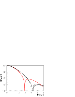
Figure 1: (Color online) The magnetic ff of ³He, $G_{M}^{3}(\Delta^{2})$. Full line: the present IA calculation, obtained as the integral of Eq. (11), summed over the flavors (see text), together with the experimental data dataff . The units used for the momentum transfer, $\Delta^{\mu}\equiv\sqrt{-\Delta^{2}}$, have been chosen for an easy comparison with the results of Ref. Marcucci:1998tb .

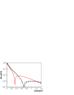
Figure 2: (Color online) As in Fig. 1, but in units of GeV², as a function of $-\Delta^{2}$.

As discussed in Ref. io , the accuracy of this calculation, since a NR spectral function is used to evaluate Eqs. (10) and (11), is of order ${\cal{O}}\left({\vec{p}\,^{2}/M^{2}},{\vec{\Delta}^{2}/M^{2}}\right)$. The interest of the present calculation is precisely that of investigating nuclear effects at low values of $\vec{\Delta}^{2}$, for which measurements in the coherent channel may be performed.

The calculation of Eq. (10) has been performed and discussed in Ref. io . It has been found that the properties $i),ii)$ of GPDs, defined above, are properly recovered. The property $iii)$, the so called polinomiality, is slightly violated at the low values of $\Delta^{2}$ and $\xi$ of interest here, due to the NR IA which is being used. The same problem affects also the evaluation of Eq. (11).

In order to evaluate Eq. (11), the quantity of interest here, one needs models of the nuclear spectral function and of the nucleon GPDs $H_{q}^{N}$ and $E_{q}^{N}$. The models used in the present calculation are described in the next section.

III Ingredients of the calculation

As stated above and as it is explained thoroughly in the Appendix B, in order to evaluate $P^{N}_{SS^{\prime},ss^{\prime}}(\vec{p},\vec{p}\,^{\prime},E)$, the spin-dependent non-diagonal spectral function of the nucleon $N$ in ³He, one needs intrinsic nuclear overlaps. These quantities have been evaluated exactly in Ref. pssk along the line of Ref. gema , using the wave function of Ref. tre corresponding to the Av18 interaction av18 , taking into account the Coulomb repulsion between the two protons. For a relevant comparison to be described later on, the calculation has been performed also using the nuclear overlaps corresponding to the Av14 interaction av14 , firstly evaluated to be used in Ref. gema , including again the Coulomb repulsion.

Concerning the model of the nucleon GPDs to be used, a preliminary observation is in order. In this paper the interest is only in the evaluation of nuclear effects, to test if the neutron dominates the nuclear observable and to suggest an extraction procedure. It is therefore important to use different models, based on different assumptions on the hadron structure, to evaluate $\tilde{G}_{M}^{3}$, and to check if the dominance of the neutron contribution, and the reliability of the extraction procedure, are valid independently of the model used. We are going therefore to use three very different models, namely:

1) the model of Ref. rad1 , which, despite of its simplicity, fulfills the general properties of GPDs. The GPD $H_{q}$ is built in agreement with the Double Distribution representation radd . The $\Delta^{2}$ dependence, factorized out from the one in $x$ and $\xi$, is given by $F_{q}(\Delta^{2})$, i.e., the contribution of the quark of flavour $q$ to the nucleon ff, obtained from the experimental values of the proton, $F_{1}^{p}$, and of the neutron, $F_{1}^{n}$, Dirac ffs (see Ref. io ). For the numerical evaluation, use has been made of the parametrization of the nucleon Dirac ff given in Ref. gari . The model has been minimally extended to parametrize also the GPD $E_{q}$, assuming that it is proportional to the charge of $q$ (this choice, a very natural one, is used, e.g., in Refs. from ). In this way, proper relations are found between the $u$ and $d$ contributions to the Pauli ff and the proton and neutron Pauli ff; again, for the latter quantities, the parametrization of Ref. gari has been used;

2) The model of GPDs described in Ref. sv , arising in a constituent quark description of the nucleon structure, performing a microscopic calculation without assuming any factorization. The model, completely different in spirit from the previously described one, refers to a low $Q^{2}$ scale and is reasonable only in the valence quark region;

3) The microscopic model calculation of Ref. song , based on a simple version of the MIT bag model, i.e., assuming confined free relativistic quarks in the nucleon, a completely different scenario with respect to the constituent quark picture and the double distribution one.

For the present aim, there is no need to use recent, sophisticated GPDs models, such as the ones of Refs. belli1 ; belli2 , which would complicate the description without adding new insights. Once the experiments are planned, more realistic calculations involving phenomenologically motivated models will be easily implemented in our scheme.

IV The neutron and proton contributions to the GPDs of ³He

Using the ingredients described above, the calculation of Eq. (11) has been performed in the nuclear Breit-frame. Unfortunately, the only safe way to establish the reliability of the approach, the comparison with experiments, is not possible. In facts, data for the GPDs are not available and, for $E_{q}^{3}$ in particular, even the forward limit is unknown. One check is in any case possible and it is therefore a crucial one: the quantity

$$\tilde{G}_{M}^{3}(x,\Delta^{2},\xi)=\sum_{q}\tilde{G}_{M}^{3,q}(x,\Delta^{2},\xi),$$ (12)

i.e., Eq. (3), summed over the active flavors, can be integrated over $x$ to give the experimentally well-known magnetic ff of ³He, $G_{M}^{3}(\Delta^{2})$ (cf. Eq. (4)). The result obtained using this procedure is in excellent agreement with the Av18 one-body calculation presented in Ref. Marcucci:1998tb , and with the non-relativistic part of the calculation in Ref. Baroncini:2008eu (see Figs. 1-2). Moreover, for the values of $\Delta^{2}$ which are relevant for the coherent process under investigation here, i.e., $-\Delta^{2}\lesssim 0.15$ GeV², our results compare well also with the data dataff . For higher values, the agreement is lost and to get a good description one should go beyond IA, including three-body forces and two-body currents (see, e.g., Marcucci:1998tb ). If measurements were performed at these values of $-\Delta^{2}$, our calculations could be improved by allowing for these effects; for the moment being, since coherent DVCS cannot be measured at $-\Delta^{2}>$ 0.15 GeV² for nuclear targets, the good description obtained close to the static point is quite satisfactory.

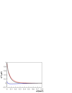
Figure 3: (Color online) The proton contribution, $G_{M}^{3,p}(\Delta^{2})$ (dot-dashed), and the neutron one, $G_{M}^{3,n}(\Delta^{2})$ (dashed), to the magnetic ff of ³He, $G_{M}^{3}(\Delta^{2})$ (full), obtained within the present IA approach.

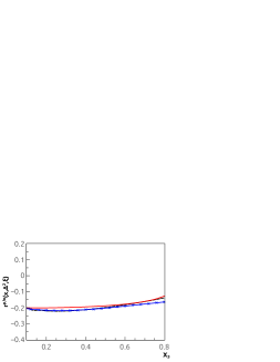
Figure 4: (Color online) The ratio of the proton to neutron contribution to the quantity $x_{3}\tilde{G}_{M}^{3}(x,\Delta^{2},\xi)$ of ³He (full), Eq. (13), obtained at $-\Delta^{2}=0.1$ GeV² and $\xi_{3}$ = 0, using the nucleon GPDs model of Ref. rad1 in Eq. (11), compared with the same ratio evaluated using the nucleon GPDs model of Ref. sv (dashed) and that of Ref. song (crosses).

With the comfort of this successful check, let us briefly recall the main outcome of Ref. nostro . In that paper, the quantity $x_{3}\tilde{G}_{M}^{3}(x,\Delta^{2},\xi)$, which, in the forward limit, yields the integrand of the JSR (cf. Eq. (5) where the relation is given for a given flavor $q$), has been presented as a function of $x_{3}$, in the forward limit and at finite values of $\Delta^{2}$ and $\xi_{3}$ (Here we have defined $x_{3}=({M_{A}/M})x$ and $\xi_{3}=({M_{A}/M})\xi$, in order to recover the standard notation used in studies of DIS off nuclei. In facts, the Bjorken variable is defined as $x_{Bj}=Q^{2}/(2M\nu)$, being $\nu=q_{0}$ in the laboratory system. It ranges naturally between 0 and ${M_{A}/M}$ for a nuclear target of mass $M_{A}$. It is therefore convenient to rescale the variables $x,\xi$ by the factor ${M_{A}/M}$).

For the nuclear GPDs, a dramatic $\Delta^{2}$ behavior, basically governed by that of the ff, has been found. This fact can be realized looking at Fig. 3, where the separate contribution of the neutron and of the protons to $G_{M}^{3}(\Delta^{2})$ is shown in linear scale. The most striking result of Ref. nostro is actually that the contribution of the neutron is impressively dominating the nuclear GPD at low $\Delta^{2}$, with the proton contribution growing fast with increasing $\Delta^{2}$. However for the flavor $d$ the impressive dominance of the neutron contribution varies slowly with increasing $\Delta^{2}$. This behavior of the $d$ contribution is explained in Ref. nostro in terms of the flavor structure of Eqs. (10) and (11).

Of course, the shape of the curves obtained for $\tilde{G}_{M}^{3}$ is very dependent on the nucleonic model used as input in the calculation, i.e., in the case of Ref. nostro , that of Ref. rad1 . One should not forget, we reiterate, that the aim of this analysis, for the moment being, is that of getting a clear estimate of the proton and neutron contributions to the nuclear observable, a feature rather independent on the nucleonic model. To demonstrate this property, we have plotted, in Fig. 4, the ratio of the proton to neutron contribution to $\tilde{G}_{M}^{3}$:

$$r^{p/n}(x,\Delta^{2},\xi)=\tilde{G}_{M}^{3,p}(x,\Delta^{2},\xi)/\tilde{G}_{M}^{3,n}(x,\Delta^{2},\xi)~{},$$ (13)

calculated using as input the $\tilde{G}^{p(n),q}_{M}$ corresponding to the model of Ref. rad1 , and those of the very different models of Refs. sv and song . The three ratios are slowly varying as a function of $x_{3}$ and are very close to each other, demonstrating the very weak model dependence of this feature of the result.

Summarizing, our IA calculation shows that, at very low $-\Delta^{2}\simeq 0.1$ GeV², there is a clear dominance of the neutron contribution on the proton one, and that such a dominance, even stronger for the $d$ flavor, does not depend on the nucleonic model used in the calculation. Anyway, a couple of items have still to be investigated: $i)$ even if the neutron contribution is dominating, the extraction of the neutron GPDs from it may be nontrivial and a proper strategy has to be studied; $ii)$ although the very low $\Delta^{2}$ values define the most interesting region, where, for example, the JSR can be checked, this region may be difficult to be reached experimentally. A procedure able to take into account the nuclear effects arising in an IA description also at higher $\Delta^{2}$ would be very helpful.

A positive answer to these two remaining problems will be given in the next section.

V Extracting the neutron information from ³He data

Let us discuss the most relevant issue.

It is convenient to rewrite our main equation, Eq. (11), in a different form, defining a variable $z$ as follows:

$$z-{M_{A}\over M}{\xi\over\xi^{\prime}} = z-{M_{A}\over M}\left[{p^{+}\over P^{+}}(1+\xi)-\xi\right]$$ (14)

$$= z+\xi_{3}-{M_{A}\over M}{p^{+}\over P^{+}}(1+\xi)$$

$$= z+\xi_{3}-{M_{A}\over M}{p^{+}\over\bar{P}^{+}}~{},$$

where use has been made of Eqs. (6) – (8). Eq. (11) can be written therefore in the form

$$\tilde{G}_{M}^{3,q}(x,\Delta^{2},\xi) = \sum_{N}\int_{x_{3}}^{M_{A}/M}{dz\over z}g_{N}^{3}(z,\Delta^{2},\xi)$$ (15)

$$\times \tilde{G}_{M}^{N,q}\left({x\over z},\Delta^{2},{\xi\over z},\right)~{},$$

where the off-diagonal spin-dependent light cone momentum distribution

$$g_{N}^{3}(z,\Delta^{2},\xi) = \int dE\int d\vec{p}\,\tilde{P}_{N}^{3}(\vec{p},\vec{p}+\vec{\Delta},E)$$ (16)

$$\times \delta\left(z+\xi_{3}-{M_{A}\over M}{p^{+}\over\bar{P}^{+}}\right)$$

has been introduced and the quantity

$$\tilde{P}_{N}^{3}(\vec{p},\vec{p}+\vec{\Delta},E) = P^{N}_{+-,+-}(\vec{p},\vec{p}\,^{\prime},E)$$ (17)

$$- P^{N}_{+-,-+}(\vec{p},\vec{p}\,^{\prime},E)~{},$$

for the sake of clarity, has been introduced.

$\Delta^{2}$	$G^{3,p,point}_{M}$	$G^{3,p,point}_{M}$	$G^{3,n,point}_{M}$	$G^{3,n,point}_{M}$
$[$GeV2$]$	Av18	Av14	Av18	Av14
0	-0.044	-0.049	0.879	0.874
-0.1	0.040	0.038	0.305	0.297
-0.2	0.036	0.035	0.125	0.119

Table 1: The proton and neutron contributions to the magnetic point like ff of ³He, corresponding to the Av18 av18 and Av14 av14 nuclear interactions, for three low values of $-\Delta^{2}$.

Let us now perform the $x-$integral of the function $\tilde{G}_{M}^{3,q}(x,\Delta^{2},\xi)$, given by Eq. (15). One obtains:

$$\int dx \,\tilde{G}_{M}^{3,q}(x,\Delta^{2},\xi)=$$ (18)

$$= \sum_{N}\int dx\int{dz\over z}g_{N}^{3}(z,\Delta^{2},\xi)\tilde{G}_{M}^{N,q}\left({x\over z},\Delta^{2},{\xi\over z}\right)=$$

$$= \sum_{N}\int dx^{\prime}\tilde{G}_{M}^{N,q}(x^{\prime},\Delta^{2},\xi^{\prime})\int dzg_{N}^{3}(z,\Delta^{2},\xi)=$$

$$= \sum_{N}G_{M}^{N,q}(\Delta^{2})\,G_{M}^{3,N,point}(\Delta^{2})$$

$$= G_{M}^{3,q}(\Delta^{2})~{}.$$

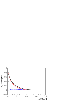
Figure 5: (Color online) The magnetic point like ff of ³He (full), given by the sum of the neutron (dashed) and proton (dot-dashed) contribution (Eq. (19)).

In the equation above, $G_{M}^{3,q}(\Delta^{2})$ is the contribution, of the quark of flavor $q$, to the nuclear ff; $G_{M}^{N,q}(\Delta^{2})$ is the contribution, of the quark of flavour $q$, to ff of the nucleon $N$; $G_{M}^{3,N,point}(\Delta^{2})$ is the so-called ³He magnetic “point like ff”, which would represent the contribution of the nucleon $N$ to the magnetic ff of ³He if $N$ were point-like. The latter quantity has a relevant role in our discussion; we stress that it is given, in the present IA approach, by

$$G_{M}^{3,N,point}(\Delta^{2}) = \int dE\int d\vec{p}\,\tilde{P}_{N}^{3}(\vec{p},\vec{p}+\vec{\Delta},E)$$ (19)

$$= \int_{0}^{M_{A}/M}dz\,g_{N}^{3}(z,\Delta^{2},\xi)~{}.$$

This quantity, obtained in our Av18 framework, is shown for $N=p,n$, and for their sum, $G_{M}^{3,point}(\Delta^{2})$ in Fig. 5. Obviously, this one-body property can be obtained from the wave function only and, at least for the low values of $\Delta^{2}$ of interest here, we checked that it depends very weakly on the nuclear interaction. In fact, we have performed the calculation using also the Av14 interaction, including the Coulomb repulsion between the protons. The curves we have obtained cannot be distinguished from the Av18 ones shown in Fig. 5 and have not been reported. The different magnetic point like ffs corresponding to the different nuclear interactions are therefore reported in Tab. 1 for three low values of $-\Delta^{2}$. Now it comes an important observation. The variable $z$, at the low values of $\Delta^{2}$ and $\xi$ which are of interest here, is very similar to the light cone ${}^{\prime\prime}+^{\prime\prime}$ momentum fraction and the function $g_{N}^{3}(z,\Delta^{2},\xi)$ very close to a standard, forward light-cone momentum distribution. Besides, the nucleon dynamics in ³He is, to a large extent, a NR one. This makes any ³He light-cone momentum distribution, polarized or unpolarized, strongly peaked around $z=1$ (see, i.e., the discussion in Ref. io ). Evaluating Eq. (24) close to $z=1$ means, as a matter of facts, that all the nuclear effects, but the ones due to the spin structure of the target, are negligible. Basically, this means that the momentum and energy distributions of the nucleons do not affect the result. If this is the case, from Eq. (15) one gets:

$$\tilde{G}_{M}^{3,q}(x,\Delta^{2},\xi) = \sum_{N}\tilde{G}_{M}^{N,q}\left(x,\Delta^{2},{\xi}\right)$$ (20)

$$\times \int_{x_{3}}^{M_{A}/M}\hskip-17.07164pt{dz}g_{N}^{3}(z,\Delta^{2},\xi)+O(z-1)$$

and, considering that, for ³He, $g_{N}^{3}(z,\Delta^{2},\xi)\simeq 0$ for $x_{3}\lesssim 1$, being this function strongly peaked around $z=1$, the lower integration limit in $z$ can be put equal to 0 for the $x_{3}$ values relevant here ($x_{3}\lesssim 0.7$). In other words, at low values of $\Delta^{2}$ and $\xi$, the following approximation of Eq. (11) should hold:

$$\tilde{G}_{M}^{3,q}(x,\Delta^{2},\xi) \simeq \sum_{N}\tilde{G}_{M}^{N,q}\left(x,\Delta^{2},{\xi}\right)$$ (21)

$$\times \int_{0}^{M_{A}/M}{dz}g_{N}^{3}(z,\Delta^{2},\xi)$$

$$= G^{3,p,point}_{M}(\Delta^{2})\,\tilde{G}_{M}^{p,q}(x,\Delta^{2},\xi)$$

$$+ G^{3,n,point}_{M}(\Delta^{2})\,\tilde{G}_{M}^{n,q}(x,\Delta^{2},\xi)~{}.$$

Clearly, in the last line, use has been made of Eq. (19). If the factorized expression above were a good approximation of Eq. (11), it would be very helpful. In facts, Eq. (21) is very simple: all the nuclear effects are hidden in the magnetic point like ffs, quantities which can be obtained directly from the wave function, without considering the complicated spectral effects described by Eq. (11); moreover, and more important, these quantities, at low $-\Delta^{2}$, are theoretically well known and, as Tab. 1 shows, depend very weakly on the used nuclear interaction.

Figs. 6 and 7 demonstrate that Eq. (21) approximates nicely the full result Eq. (11) in the kinematics of interest here, the two quantities differing of few percents at most for $x_{3}<0.7$. This is an important point: Eq. (21) can now be solved to extract the neutron GPD $\tilde{G}_{M}^{n}$:

$$\tilde{G}_{M}^{n,extr}(x,\Delta^{2},\xi) \simeq {1\over G^{3,n,point}_{M}(\Delta^{2})}\left\{\tilde{G}_{M}^{3}(x,\Delta^{2},\xi)\right.$$ (22)

$$- \hskip-5.69054pt\left.G^{3,p,point}_{M}(\Delta^{2})\tilde{G}_{M}^{p}(x,\Delta^{2},\xi)\right\},$$

an equation which could be used to obtain the neutron information from ³He, $\tilde{G}_{M}^{3}$, and proton, $\tilde{G}_{M}^{p}$, data, simply correcting by means of the well known magnetic point like ffs.

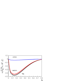
Figure 6: (Color online) The quantity $x_{3}\tilde{G}_{M}^{3}(x,\Delta^{2},\xi)$ of ³He in the forward limit, together with the proton and neutron contribution (full lines), compared with the approximations to these quantities given by the factorized form Eq. (21) (dashed lines).

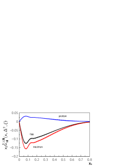
Figure 7: (Color online) The same as in Fig. 6, but at $\Delta^{2}=-0.1$ GeV² and $\xi_{3}=0.1$.

We have checked the validity of the proposed extraction procedure by evaluating Eq. (22), using for the magnetic point like ffs the ones corresponding the Av18 interaction, for the proton GPD $\tilde{G}_{M}^{p}$ the one given by the model rad1 , for $\tilde{G}_{M}^{3}$ the one calculated by means of Eq. (11), i.e., we are simulating ³He data by using our best calculation. If the extraction procedure were able to describe exactly, in an effective way, the nuclear corrections predicted in IA, the obtained $\tilde{G}_{M}^{n,extr}$ should be equal to the neutron quantity, $\tilde{G}_{M}^{n}$, used as input in the calculation, i.e., again, the one predicted for the neutron by the model of Ref. rad1 .

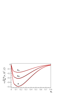
Figure 8: (Color online) The quantity $x_{3}\tilde{G}_{M}^{n,q}(x,\Delta^{2},\xi)$ for the neutron in the forward limit, evaluated in the model of Ref. rad1 and labelled $n$, given by the sum of the $u$, labelled $n_{u}$, and $d$, labelled $n_{d}$ contribution (full lines), compared with the approximations to these quantities given by Eq. (22) (dashed lines) (see text).

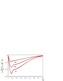
Figure 9: (Color online) The same as in Fig. 8, but at $\Delta^{2}=-0.1$ GeV² and $\xi_{3}=0.1$.

Figs. 8 and 9 demonstrate that these two quantities, and the $u$ and $d$ flavor contribution to them, differ at most by few percents in all the relevant kinematical range. This means that the growth of the proton contribution to the ³He observable, which seemed to hinder the extraction of the neutron information, in particular for the $u$ flavor, is governed by the $-\Delta^{2}$ behavior of the magnetic point like ffs, quantities which are under theoretical control. By using them, the extraction of the neutron GPDs, close to the forward limit, is safe and basically model independent.

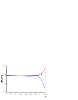
Figure 10: (Color online) The ratio Eq. (23), in the forward limit (full), at $\Delta^{2}=-0.1$ GeV² and $\xi_{3}=0$ (dashed) and at $\Delta^{2}=-0.1$ GeV² and $\xi_{3}=0.1$ (dot-dashed).

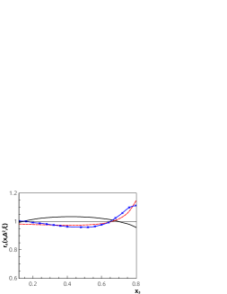
Figure 11: (Color online) The ratio Eq. (23), at $\Delta^{2}=0.1$ GeV² and $\xi_{3}=0$, using, to evaluate Eq. (11), for the nucleon GPDs, the model of Ref. rad1 (dashed), the one of Ref. sv (full) and that of Ref. song (crosses).

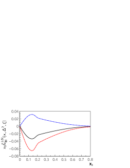
Figure 12: (Color online) The quantity $x_{3}\tilde{G}_{M}^{3}(x,\Delta^{2},\xi)$, at $\Delta^{2}=-0.2$ GeV² and $\xi_{3}=0.2$ (full), together with the neutron (dashed) and the proton (dot-dashed) contribution.

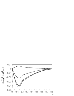
Figure 13: The quantity $x_{3}\tilde{G}_{M}^{3,q}(x,\Delta^{2},\xi)$ for the $d$ (full) and $u$ (dot-dashed) flavor, at $\Delta^{2}=-0.2$ GeV², and $\xi_{3}$=0.2. The neutron contributions for the $d$ (dashed) and $u$ (long-dashed) flavor are also shown.

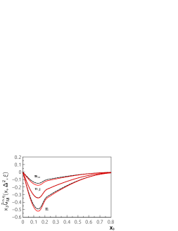
Figure 14: (Color online) The same as in Fig. 8, but at $\Delta^{2}=-0.2$ GeV² and $\xi_{3}=0.2$.

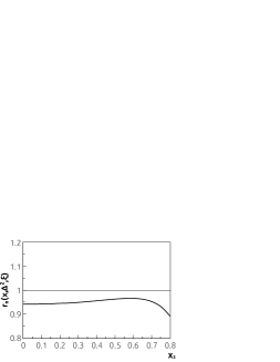
Figure 15: The same as in Fig. 10, but at $\Delta^{2}=-0.2$ GeV² and $\xi_{3}=0.2$.

These feature is even more evident in Fig. 10, where the ratio

$$r_{n}(x,\Delta^{2},\xi)=\tilde{G}_{M}^{n,extr}(x,\Delta^{2},\xi)/\tilde{G}_{M}^{n}(x,\Delta^{2},\xi)~{},$$ (23)

is shown. Obviously, this ratio would be one in case the extraction procedure were working perfectly. It is clear that, in all the relevant kinematics, the extraction procedure takes into account the nuclear effects introduced in the IA analysis for $x_{3}\lesssim 0.7$ with an accuracy of a few percents.

Besides, the quality of the extraction does not depend on the nucleonic model used. In Fig. 11, in one particular kinematics, it is shown the ratio $r_{n}$, Eq. (23), obtained using the three different models of GPDs considered in this work, i.e. the ones of Refs. rad1 ; sv ; song . It is clearly seen that the procedure works within a few percent accuracy, independently on the model used.

Let us show now that the technique works at higher $-\Delta^{2}$ values. Figs. 12-15 are devoted to show this fact. All the steps are repeated, in a sort of useful summary of the procedure. In Fig. 12, the proton and neutron contributions to ³He are shown at $\Delta^{2}=-0.2$ GeV² and $\xi_{3}=0.2$, and they are found to be comparable in size; in Fig. 13, it is shown that this problem is serious, in particular, for the $u$ flavor. In Fig. 14 and 15 the good quality of the extraction procedure is demonstrated even in this less forward situation, by showing the extracted neutron GPD and its ratio to the model used as input in the calculation, respectively. This is a good piece of news for the experimental programme, in case that extremely small values of $-\Delta^{2}$ could not be reached. However, we reiterate that the very good extraction scheme is really useful where IA provides a reasonable description of the process, a region which coincides with $-\Delta^{2}\lesssim 0.15$ GeV².

Another feature of the IA used here is the assumption that only nucleonic degrees of freedom are considered in the analysis, and that the nucleon structure is not modified by the nuclear medium. The study of possible modifications, i.e. the study of “off-shell” effects, is certainly a relevant issue and it would deserve dedicated investigations, beyond the scope of the present paper. We note however that careful analyses of these effects for different targets, performed, e.g., in Ref. liuti3 for ⁴He, show that they grow with $\Delta^{2}$, being minimal close to the forward limit, where we are proposing the relevant measurement.

In closing this section, let us mention that another process to access the neutron GPDs is incoherent DVCS off the neutron in nuclear targets, i.e., the process with the struck neutron detected in the final state, in coincidence with the scattered electron and the produced photon. An experiment of this type will be performed at the 12 GeV program of JLab silvia for a ²H target. We plan therefore to investigate also incoherent DVCS off the neutron in ³He, although these kind of processes could be spoiled by Final State Interactions of the detected neutron.

VI Conclusions

In this work we have thoroughly described an IA calculation of the GPDs $H_{q}$ and $E_{q}$ of ³He. In proper limits, the correct constraints are recovered. Coherent DVCS off ³He at low $\Delta^{2}$ turns out to be strongly dominated by the neutron contribution, in particular for the $d$ flavor, from which the neutron information has to be extracted. A procedure has been described to take into account the nuclear effects included in the IA analysis and to safely disentangle the neutron information from them, even at moderate values of the momentum transfer. The only theoretical nuclear ingredients are the neutron and proton contributions to the magnetic point like form factors of ³He, quantities which are under good theoretical control at low momentum transfer and that encode correctly all the nuclear effects described in an IA framework. If high values of $\Delta^{2}$ were reached, the IA description would not be reliable and two-body currents and three-body forces would have to be included into the approach. We have checked that the dominance of the neutron contribution and the proposed extraction procedure do not depend on the model of the nucleon GPD used in the calculation. Our results confirm strongly coherent DVCS off ³He at low momentum transfer as a key experiment to access the neutron GPDs. It will be very interesting and useful to perform a Light-Front analysis of the process, which already started in SiDIS alessio , so to have, from the beginning, a relativistic framework for the investigation.

Appendix A GPDs from the components of the light cone correlator

In this work, both the nucleus, being the relevant momentum transfer low, and the nucleon, whose dynamics is governed by the Schrödinger equation, are treated non-relativistically (NR). A NR expression of the spinors appearing in Eq. (1) has therefore to be used, in order to find explicit relations between the correlator $F^{q,A,\mu}_{s^{\prime}s}$, Eq. (1), and the GPDs.

In the NR limit one has (see, e.g., ps ):

$$u(p,s)=\left(\begin{array}[]{c}\sqrt{p\cdot\sigma}\chi_{s}\\ \sqrt{p\cdot\overline{\sigma}}\chi_{s}\end{array}\right)\underset{N.R}{\longrightarrow}\sqrt{m}\left(\begin{array}[]{c}\left(1-\dfrac{\overrightarrow{p}\overrightarrow{\sigma}}{2m}\right)\chi_{s}\\ \left(1+\dfrac{\overrightarrow{p}\overrightarrow{\sigma}}{2m}\right)\chi_{s}\end{array}\right)~{},$$ (28)

and:

$$\overline{u}(p^{\prime},s^{\prime})\gamma^{0}u(p,s) \approx 2m\chi_{s^{\prime}}^{\dagger}\chi_{s}~{},$$

$$\overline{u}(p^{\prime},s^{\prime})\gamma^{i}u(p,s) \approx 2m\chi_{s^{\prime}}^{\dagger}\left(\dfrac{-i}{2m}\varepsilon^{ijk}\Delta_{j}\sigma_{k}\right)\chi_{s}~{},$$

$$\overline{u}(p^{\prime},s^{\prime})\left(\dfrac{i}{2m}\sigma^{i\nu}\Delta_{\nu}\right)u(p,s) \approx 2m\chi_{s^{\prime}}^{\dagger}\left(\dfrac{-i}{2m}\varepsilon^{ijk}\Delta_{j}\sigma_{k}\right)\chi_{s}~{}.$$ (29)

Properly choosing the components of $\gamma^{\mu}$, it is possible to find the most convenient relation between $F_{s^{\prime}s}^{q,A,\mu}$ and the GPDs. By taking for $\chi$ the eigenstates of $\sigma^{3}$, being $z$ the quantization axis, fixing $\mu=0$, one obtains:

$$F_{++}^{q,A,0}(x,\Delta^{2},\xi) = \dfrac{m}{2\overline{p}^{+}}H_{q}^{A}(x,\Delta^{2},\xi)$$

$$F_{--}^{q,A,0}(x,\Delta^{2},\xi) = F_{++}^{q,A,0}(x,\Delta^{2},\xi)~{},$$

$$F_{-+}^{q,A,0}(x,\Delta^{2},\xi) = F_{+-}^{q,A,0}(x,\Delta^{2},\xi)=0~{}.$$ (30)

In the same way, for $\mu=1$ one gets

$$F_{++}^{q,A,1}(x,\Delta^{2},\xi) = 0~{},$$

$$F_{--}^{q,A,1}(x,\Delta^{2},\xi) = F_{++}^{q,A,1}(x,\Delta^{2},\xi)~{},$$

$$F_{-+}^{q,A,1}(x,\Delta^{2},\xi) = -F_{+-}^{q,A,1}(x,\Delta^{2},\xi)=-\dfrac{\Delta_{z}}{2\overline{p}^{+}}\tilde{G}_{M}^{A,q}(x,\Delta^{2},\xi)~{}.$$ (31)

Collecting all the above results, one has

$$H_{q}^{A}(x,\Delta^{2},\xi) = \dfrac{\overline{p}^{+}}{m}F_{++}^{q,A,0}(x,\Delta^{2},\xi)~{},$$

$$\tilde{G}_{M}^{A,q}(x,\Delta^{2},\xi) = \dfrac{2\overline{p}^{+}}{\Delta_{z}}F_{-+}^{q,A,1}(x,\Delta^{2},\xi)~{},$$ (32)

which coincides with Eq. (II).

Appendix B The light cone correlator from nuclear overlaps in IA

The relevant nuclear structure quantity in the present calculation is the spin-dependent non-diagonal spectral function of the nucleon $N$ in ³He:

$$P^{N}_{SS^{\prime},ss^{\prime}}(\vec{p},\vec{p}\,^{\prime},E) = \dfrac{1}{(2\pi)^{6}}\dfrac{M\sqrt{ME}}{2}\int d\Omega_{t}$$

$$\times \sum_{\begin{subarray}{c}s_{t}\end{subarray}}\langle\vec{P^{\prime}}\,S^{\prime}|\vec{p}\,^{\prime}s^{\prime},\vec{t}\,s_{t}\rangle_{N}\langle\vec{p}\,s,\vec{t}\,s_{t}|\vec{P}\,S\rangle_{N}~{},$$

and the most important ingredient appearing in the definition Eq. (B) is the intrinsic overlap integral

$$\langle\vec{p}\,s,\vec{t}\,s_{t}|\vec{P}\,S\rangle_{N}=\int d\vec{y}\,e^{i\vec{p}\cdot\vec{y}}\langle\chi^{s}_{N},\Psi_{t}^{s_{t}}(\vec{x})|\Psi_{3}^{S}(\vec{x},\vec{y})\rangle~{}$$ (34)

between the wave function of ³He, $\Psi_{3}^{S}$, with the final state, described by two wave functions. One of them is the eigenfunction $\Psi_{t}^{s_{t}}$, with eigenvalue $E=E_{min}+E_{R}^{*}$, of the state $s_{t}$ of the intrinsic Hamiltonian pertaining to the system of two interacting nucleons with relative momentum $\vec{t}$, which can be either a bound or a scattering state. The other one is the plane wave representing the nucleon $N$ in IA.

The overlap Eq.(34) is therefore the crucial nuclear ingredient to evaluate the light cone correlator, Eq.(1), for ³He. Let us show how it is obtained through the quantity at our disposal, which is actually the following:

$$\tilde{{I}}^{X,j_{12},\eta}_{L_{\rho}{\tau},\Sigma}(y_{1},E) = \int d\Omega_{\hat{y}_{1}}~{}\sum_{M_{\rho},M_{X}}\langle XM_{X},L_{\rho}M_{\rho}|{1\over 2}J_{z}\rangle~{}{Y}^{*}_{L_{\rho}M_{\rho}}(\Omega_{\hat{y}_{1}})\left[{\cal T}_{1\over 2}^{\tau}\right]^{\dagger}~{}$$ (35)

$$\times \sum_{m_{12}\sigma}\langle j_{12}m_{12},{1\over 2}\sigma|XM_{X}\rangle\langle{\bf y}_{1},{1\over 2}\sigma;\psi^{j_{12},m_{12},\Sigma}_{E,\eta}|\Psi_{{}^{3}He}^{{1\over 2}J_{z}}\rangle\ .$$

Here above, $\rho$ denotes quantum numbers of the struck nucleon, treated as a free particle in IA, with spin projection $\sigma$, isospin projection $\tau$, orbital angular momentum and its third component $L_{\rho},~{}M_{\rho}$, respectively. $\psi^{j_{12},m_{12}\Sigma}_{E,\eta}$ represents the two-body recoiling system with total angular momentum and its third component $j_{12},~{}m_{12}$, spin $\Sigma$ and excitation energy $E$. $\eta$ is an additional quantum number necessary to describe the OAM mixing in the interacting two-body state in the continuum. $j_{12}$ is coupled to the spin $\frac{1}{2}$ of the interacting nucleon to give the intermediate angular momentum $X$. The description of the three-body system is based on the Av18 calculation of the wave function of Ref. tre , given in terms of the following Jacobi coordinates ${\bf y}_{1}$ and ${\bf x}_{1}$:

$${\bf y}_{1} = -{2\over\sqrt{3}}~{}\left[\bf{r}_{1}-{\bf{r}_{2}+\bf{r}_{3}\over 2}\right]=-{2\over\sqrt{3}}~{}{\mbox{\boldmath$\rho$\/}}$$

$${\bf x}_{1} = \left[\bf{r}_{2}-\bf{r}_{3}\right]={\bf r}$$ (36)

where ${\bf r}_{i}$ (with $i=1,2,3$) are the CM variables of the nucleons in the trinucleon, constrained by ${\bf r}_{1}+{\bf r}_{2}+{\bf r}_{3}=0$. The trinucleon bound state, $\Psi_{{}^{3}He}^{\frac{1}{2}J_{z}}({\bf x}_{1},{\bf y}_{1})$, can be written in terms of the variables ${\bf y}_{1}$ and ${\bf x}_{1}$ using the following basis for the isospin-spin-angular part:

$${\cal Y}^{J_{12}\Sigma\ell_{12}}_{L_{\rho}XJJ_{z}}(\hat{x}_{1},\hat{y}_{1}) = \sum_{M_{\rho}M_{X}}\sum_{m_{12}\sigma}\langle j_{12}M_{12},{1\over 2}\sigma|XM_{X}\rangle\langle XM_{X},L_{\rho}M_{\rho}|\frac{1}{2}J_{z}\rangle$$ (37)

$$\times \sum_{m_{12}}\sum_{\mu}~{}\chi_{\Sigma}^{\mu}~{}{Y}_{\ell_{12}m_{12}}(\Omega_{{\hat{x}}_{1}})~{}\langle\ell_{12}m_{12},{\Sigma}\mu|j_{12}M_{12}\rangle~{}$$

$$\times \sum_{\tau\tau_{12}}\langle{1\over 2}\tau,T_{12}\tau_{12}|\frac{1}{2}\frac{1}{2}\rangle~{}{\cal T}_{1\over 2}^{\tau}~{}{\cal T}_{T_{12}}^{\tau_{12}}{Y}_{L_{\rho}M_{\rho}}(\Omega_{{\hat{y}}_{1}})\chi_{1\over 2}^{\sigma}$$

through the radial overlaps

$$\tilde{{\cal I}}^{j_{12}\Sigma\ell_{12}}_{L_{\rho}X}(|{\bf x}_{1}|,|{\bf y}_{1}|)=\int d\Omega_{{\hat{y}}_{1}}\int d\Omega_{{\hat{x}}_{1}}\left[{\cal Y}^{j_{12}\Sigma\ell_{f}}_{L_{\rho}XJJ_{z}}(\hat{x}_{1},\hat{y}_{1})\right]^{\dagger}\Psi_{{}^{3}He}^{\frac{1}{2}J_{z}}({\bf x}_{1},{\bf y}_{1})$$ (38)

with the constraints

$$(-1)^{\ell_{f}+L_{\rho}}=1~{},$$

$$(-1)^{\ell_{f}+\Sigma+T_{12}}=-1\;\;,$$ (39)

following from the parity of the nucleus and the Pauli principle, respectively.

The quantity at our disposal, Eq. (35), can be defined in terms of the overlaps Eq. (39), as follows:

$$\tilde{{I}}^{X,j_{12},\eta}_{L_{\rho}{\tau},\Sigma}(y_{1},E) = \langle{1\over 2}\tau,T_{12}\tau_{12}|\frac{1}{2}\frac{1}{2}\rangle~{}\sum_{\ell_{12}}~{}\int~{}{\tilde{{\cal I}}}^{j_{12}\Sigma\ell_{12}}_{L_{\rho}X}(|{\bf y}_{1}|,|{\bf x}_{1}|)~{}u^{j_{12},E,\eta}_{\ell_{12}}(x_{1})~{}x_{1}^{2}~{}dx_{1}~{},$$ (40)

where $u^{j_{12},E,\eta}_{\ell_{12}}(x_{1})$ is the two-nucleon radial function.

Using this formalism to calculate the spectral function, Eq. (B), one has to obtain the product of two intrinsic overlaps, integrated over the angles of $\vec{t}$, the relative momentum of the recoiling pair. This quantity is expressed through the overlaps Eq. (40) which, as previously said, are the quantities at disposal, as follows:

$$\int d\Omega_{t}\langle\vec{P}^{\prime}S^{\prime}|\vec{t}s_{t},\vec{p}\,^{\prime}s^{\prime}\rangle\langle\vec{p}\,s,\vec{t}\,s_{t}|\vec{P}\,S\rangle=$$ (41)

$$= \int d\Omega_{t}\int d\rho^{\prime}e^{-i\vec{p}\,^{\prime}\vec{\rho^{\prime}}}\int d\rho e^{i\vec{p}\vec{\rho}}\langle\rho,\frac{1}{2}s;\psi^{j_{12},m_{12}\Sigma}_{E,\eta}|\Psi^{\frac{1}{2}J_{z},\frac{1}{2}T_{z}}_{{}^{3}He}\rangle$$

$$\times \langle\Psi_{{}^{3}He}^{\frac{1}{2}J^{\prime}_{z},\frac{1}{2}T_{z}}|\psi_{E,\eta}^{j^{\prime}_{12},m^{\prime}_{12}},\frac{1}{2}s^{\prime},\rho^{\prime}\rangle\left[\tau^{\tau}_{\frac{1}{2}}\right]^{\dagger}\left[\tau^{\tau}_{\frac{1}{2}}\right]=$$

$$= \int d\rho^{\prime}e^{-i\vec{p}\,^{\prime}\vec{\rho^{\prime}}}\int d\rho e^{i\vec{p}\vec{\rho}}\sum_{X,M_{X}}\sum_{X^{\prime},M_{X^{\prime}}}\sum_{m_{12},s}\sum_{s^{\prime}}\mathit{Y}^{\ast}_{L,M}(\Omega_{\rho})\mathit{Y}_{L^{\prime},M^{\prime}}(\Omega_{\rho^{\prime}})$$

$$\times \langle XM_{X},L,M|\frac{1}{2}J_{z}\rangle\langle j_{12}m_{12},\frac{1}{2}s|XM_{X}\rangle\langle J^{\prime}_{z}\frac{1}{2}|L^{\prime}M^{\prime},X^{\prime}M_{X^{\prime}}\rangle$$

$$\times \langle X^{\prime}M_{X^{\prime}}|\frac{1}{2}s^{\prime},j_{12}^{\prime}m_{12}\rangle\tilde{I}^{\Sigma,X,j_{12},T_{12},\zeta}_{L,\tau}(\rho,E)\tilde{I}^{\Sigma,X^{\prime},j_{12},T_{12},\zeta}_{L^{\prime},\tau}(\rho^{\prime},E)$$

Using these relations, together with Clebsch-Gordan coefficients and spherical harmonics properties, the final expressions for the relevant components of the light cone correlator are found:

$$F_{++}^{3,q,0}(x,\xi,\Delta^{2}) = \dfrac{M}{(2\pi)^{5}}\sum_{N}\int_{0}^{\infty}dE\sqrt{ME}\int_{0}^{\infty}dp\ p^{2}\sum_{L_{\rho},j_{12},X,\Sigma}$$ (42)

$$\times \int d\rho\ \rho^{2}j_{L_{\rho}}(p\rho)\tilde{I}_{L_{\rho},\tau}^{\Sigma,X,j_{12},T_{12}}(\rho,E)$$

$$\times \int_{-1}^{1}d\mathit{cos\theta}_{p}\int_{0}^{2\pi}d\phi_{p}P_{L_{\rho}}(\mathit{cos\theta}_{(\vec{p}+\vec{\Delta}\widehat{)}\vec{p}})$$

$$\times \int d\rho^{\prime}\rho^{\prime 2}j_{L_{\rho}}(|\vec{p}+\vec{\Delta}|\rho^{\prime})\tilde{I}_{L_{\rho},\tau}^{\Sigma,X,j_{12},T_{12}}(\rho^{\prime},E)F_{++}^{N,q,0}(x^{\prime},\xi^{\prime},\Delta^{2})\ .$$

$$F_{+-}^{3,q,1}(x,\xi,\Delta^{2}) = \dfrac{M}{(2\pi)^{4}}\sum_{N}\sum_{\begin{subarray}{c}\gamma^{\prime}\end{subarray}}\int dE\dfrac{\sqrt{ME}}{2}\int d\vec{p}\int d\rho\rho^{2}\int d\rho^{\prime}\rho^{\prime 2}$$ (43)

$$\times j_{L_{\rho^{\prime}}}(|p+\Delta|\rho^{\prime})j_{L_{\rho}}(p\rho)\tilde{I}_{\begin{subarray}{c}\beta^{\prime}\end{subarray}}(\rho^{\prime},t)\tilde{I}_{\begin{subarray}{c}\beta\end{subarray}}(\rho,t)\mathit{Y}_{L_{\rho}M_{\rho}}(\Omega_{p})(-1)^{L_{\rho^{\prime}}+\frac{L_{\rho^{\prime}}+L_{\rho}}{2}}$$

$$\times (F_{\begin{subarray}{c}\varrho\end{subarray}}\mathit{Y}^{\ast}_{L_{\rho^{\prime}},M_{\rho}-2}(\Omega_{p+\Delta})-D_{\begin{subarray}{c}\varrho\end{subarray}}\mathit{Y}^{\ast}_{L_{\rho^{\prime}},M_{\rho}}(\Omega_{p+\Delta}))F_{+-}^{N,q,1}(x^{\prime},\xi^{\prime},\Delta^{2})$$

where $\gamma^{\prime}=L_{\rho},M_{\rho},X,j_{12},\Sigma,\lambda,L_{\rho^{\prime}},X^{\prime}$. $F_{\begin{subarray}{c}\varrho\end{subarray}}$ and $D_{\begin{subarray}{c}\varrho\end{subarray}}$ are terms containing the product of four Clebsch-Gordan coefficients, depending on the set of quantum numbers $\varrho=L_{\rho^{\prime}}L_{\rho},M_{\rho},X,X^{\prime},J_{12}$.

Using the latter two equations in Eqs. (II), the nuclear GPDs, Eqs. (10) and (11), can be written through the overlaps at our disposal and, eventually, numerically evaluated.

References

- (1) D. Mueller et al., Fortsch. Phys. 42, 101 (1994) [hep-ph/9812448].
- (2) A. V. Radyushkin, Phys. Lett. B 380, 417 (1996); Phys. Rev. D 56, 5524 (1997).
- (3) X. -D. Ji, Phys. Rev. Lett. 78, 610 (1997); Phys. Rev. D 55, 7114 (1997).
- (4) M. Burkardt, Phys. Rev. D 62, 071503 (2000) [Erratum-ibid. D 66, 119903 (2002)].
- (5) M. Vanderhaeghen, P. A. M. Guichon and M. Guidal, Phys. Rev. D 60 (1999) 094017.
- (6) HERMES Collaboration, A. Airapetian et al., Nucl. Phys. B 829, 1 (2010); Phys. Rev. C 81, 035202 (2010); M. Mazouz et al., (JLab Hall A), Phys. Rev. Lett. 99, 242501 (2007).
- (7) M. Guidal, Phys. Lett. B 693, 17 (2010); Phys. Lett. B 689, 156 (2010).
- (8) E. R. Berger, et al. Phys. Rev. Lett. 87 (2001) 142302.
- (9) A. Kirchner and D. Mueller, Eur. Phys. J. C 32 (2003) 347.
- (10) V. Guzey and M. Strikman, Phys. Rev. C 68, 015204 (2003).
- (11) F. Cano and B. Pire, Eur. Phys. J. A 19 (2004) 423.
- (12) S. Liuti and S. K. Taneja, Phys. Rev. C 72 (2005) 032201.
- (13) S. Liuti and S. K. Taneja, Phys. Rev. D 70 (2004) 074019.
- (14) S. Liuti and S. K. Taneja, Phys. Rev. C 72 (2005) 034902.
- (15) V. Guzey, Phys. Rev. C 78, 025211 (2008); V. Guzey, A. W. Thomas and K. Tsushima, Phys. Lett. B 673 (2009) 9.
- (16) M. V. Polyakov, Phys. Lett. B 555 (2003) 57; V. Guzey and M. Siddikov, J. Phys. G G 32 (2006) 251; H. -C. Kim, P. Schweitzer and U. Yakhshiev, arXiv:1205.5228 [hep-ph].
- (17) J. J. Aubert et al. [European Muon Collaboration], Phys. Lett. B 123, 275 (1983).
- (18) S. Scopetta, Phys. Rev. C 70 (2004) 015205; Phys. Rev. C 79 (2009) 025207.
- (19) M. Rinaldi and S. Scopetta, Phys. Rev. C 85, 062201(R) (2012).
- (20) J. L. Friar, B. F. Gibson, G. L. Payne, A. M. Bernstein and T. E. Chupp, Phys. Rev. C 42 (1990) 2310.
- (21) C. Ciofi degli Atti, S. Scopetta, E. Pace and G. Salmè, Phys. Rev. C 48 (1993) 968.
- (22) R. -W. Schulze and P. U. Sauer, Phys. Rev. C 48, 38 (1993).
- (23) M. Diehl, Phys. Rept. 388, 41 (2003).
- (24) A.V. Belitsky and A.V. Radyushkin, Phys. Rept. 418, 1 (2005).
- (25) S. Boffi and B. Pasquini, Riv. Nuovo Cim. 30, 387 (2007).
- (26) S. K. Taneja, K. Kathuria, S. Liuti and G. R. Goldstein, Phys. Rev. D 86 (2012) 036008.
- (27) L. L. Frankfurt and M. I. Strikman, Phys. Rept. 76 (1981) 215; Phys. Rept. 160 (1988) 235.
- (28) E. Pace, G. Salmè, S. Scopetta and A. Kievsky, Phys. Rev. C 64 (2001) 055203.
- (29) A. Kievsky, E. Pace, G. Salmè and M. Viviani, Phys. Rev. C 56, 64 (1997).
- (30) A. Kievsky, M. Viviani and S. Rosati, Nucl. Phys. A 577 (1994) 511.
- (31) R. B. Wiringa, V. G. J. Stoks and R. Schiavilla, Phys. Rev. C 51 (1995) 38.
- (32) R. B. Wiringa, R. A. Smith and T. L. Ainsworth, Phys. Rev. C 29, 1207 (1984).
- (33) I. V. Musatov and A. V. Radyushkin, Phys. Rev. D 61 (2000) 074027.
- (34) A. V. Radyushkin, Phys. Lett. B 449, 81 (1999).
- (35) M. Gari and W. Krumpelmann, Phys. Lett. B 173, 10 (1986).
- (36) M. Diehl, Th. Feldmann, R. Jakob and P. Kroll, Eur. Phys. J. C 39, 1 (2005); M. Guidal, M. V. Polyakov, A. V. Radyushkin and M. Vanderhaeghen, Phys. Rev. D 72, 054013 (2005).
- (37) S. Scopetta and V. Vento, Eur. Phys. J. A 16, 527 (2003).
- (38) X. -D. Ji, W. Melnitchouk and X. Song, Phys. Rev. D 56 (1997) 5511.
- (39) G. R. Goldstein, J. O. Hernandez and S. Liuti, Phys. Rev. D 84 (2011) 034007.
- (40) D. Mueller and D. S. Hwang, PoS QNP 2012 (2012) 059.
- (41) L. E. Marcucci, D. O. Riska and R. Schiavilla, Phys. Rev. C 58, 3069 (1998).
- (42) F. Baroncini, A. Kievsky, E. Pace and G. Salmè, AIP Conf. Proc. 1056 (2008) 272.
- (43) A. Amroun, V. Breton, J. M. Cavedon, B. Frois, D. Goutte, F. P. Juster, P. Leconte and J. Martino et al., Nucl. Phys. A 579, 596 (1994).
- (44) JLab Exp. E1211003, Spokesperson: S. Niccolai.
- (45) S. Scopetta, A. Del Dotto, E. Pace, G. Salmè, Il Nuovo Cimento C, 35, 101 (2012).
- (46) M.E. Peskin, D.V. Schroeder, “An introduction to Quantum Field Theory”, Addison-Wesley Advanced Book Program, New York, 1994.