Limits on Quantum Probability Rule by no-Signaling Principle

Abstract

We have studied the possibility of post-quantum theories more nonlocal than the (standard) quantum theory using the modification of the quantum probability rule under the no-signaling condition. For this purpose we have considered the situation that two spacelike separate parties Alice and Bob share an entangled two qubit system. We have modified the quantum probability rule as small as possible such that the first local measurements are governed by the usual Born rule and the second measurement by the modified quantum probability rule. We have shown that only the maximally entangled states can have higher nonlocality than the quantum upper bound while satisfying the no-signaling condition. This fact could be a partial explanation for why the nonlocality of the quantum theory is limited. As a by-product we have found the systematic way to obtain a variety of nonlocal boxes.

1 Introduction

Quantum mechanics is nonlocal in the sense that no local hidden variable theories can simulate quantum mechanical correlations [1]. The nonlocality of quantum mechanics can be demonstrated by a violation of inequalities on measurable correlations. In the Clauser-Horne-Shimony-Holt (CHSH) inequality the degree of violation is represented by the value of the CHSH parameter $\mathcal{B}$ [2]. The quantum upper bound of $\mathcal{B}$, the degree of nonlocality, is known as Tsirelson’s bound $\mathcal{B}=2\sqrt{2}$ [3]. The nonlocality of quantum mechanics, however, is not maximum as found by Popescu and Rohrlich [4]. They derived “superquantum” correlation by using two axioms of nonlocality and relativistic causality. The maximum value $4$ of $\mathcal{B}$ is obtained for Popescu-Rohrlich (PR) nonlocal boxes [4]. The nonlocality of the PR box is limited only by the no-signaling principle whereby no information can be transferred faster than the speed of light. Therefore we naturally ask a question on the possibility of the existence of modified quantum theories, so called post-quantum theories, which are more nonlocal than the quantum theory and limited only by the no-signaling principle.

The properties of post-quantum theories are studied by several authors in an information theoretic view [5, 6, 7, 8, 9, 10, 11, 12, 13, 14, 15, 16]. As far as we know, however, there is no approach to find post-quantum theories by extending the quantum theory directly. The main postulates of the quantum theory are consisted of two parts. One is for a system and a time evolution of the system, which is based on a ray in a Hilbert space and a unitary evolution operator [17]. The other is for a measurement interpretation. Hilbert space based description of physical states is natural for a linear quantum mechanics. Projective measurement postulate, however, is justified only by experiments. The study on the possibility of higher-path interferences than two-path interference which corresponds to the generalization of the Born rule has been done both in theories and in experiments [18, 19, 20]. Therefore modifications of measurement postulates are good candidates for extending the quantum mechanics to more nonlocal post-quantum mechanics.

In the present paper, we treat the problem to find the possibility of post-quantum theories by asking a question of simulating the PR box by modifications of quantum probability postulate for quantum measurements. The standard quantum probability rule known as the Born rule is considered to be restricted by Gleason’s theorem [21]. Gleason’s theorem states that the only consistent probability assignment for all projection operators on Hilbert spaces dimension at least three must follow the standard quantum probability rule. In our study we will consider an entangled state which lives in 4-dimensional Hilbert space, therefore, it seems the modification of the Born rule is prohibited by Gleason’s theorem in simple-minded consideration, however, in our bipartite system only the local projection operators for each party are allowed. On the other hand, to prove Gleason’s theorem all possible projection operators including the global operators must be involved. Moreover, the noncontextuality of probability induced by Gleason’s propositions is lack of physical basis. We impose the no-signaling condition instead of the noncontextuality which is compatible with the relativity on the Hilbert space formalism of the physical states. We will organize this paper as follows. We will explain the formalism of the modification of the Born rule in section 2. In section 3 we will show the joint probability distribution of the PR box can be simulated by the maximally entangled state under the modified Born rule. In section 4 we will study the nonlocality of other nonlocal boxes which can be obtained systematically by changing the observables and the quantum probability rule. In section 5 we will summarize our results and discuss the implications of the results.

2 The formalism for the modification of the Born rule

In our study, we assume that a physical state is described by a vector $|\psi\rangle$ in a Hilbert space with usual norm $|\psi|=\langle\psi|\psi\rangle^{1/2}$. A physical observable is represented by a linear and Hermitian operator $\mathcal{A}$. An observable $\mathcal{A}$ has real eigenvalues $\{a_{1},\cdots,a_{d}\}$ and mutually orthonormal eigenvectors $\{|\phi_{1}\rangle,\cdots,|\phi_{d}\rangle\}$, where $d$ is the dimension of the Hilbert space. Physical observables satisfy the following measurement postulates: i) an outcome of measurement is always an eigenvalue of $\mathcal{A}$. ii) The probability of an outcome $a_{k}$ for an initial state $|\psi\rangle$ is obtained with $f(a_{k})=|\langle\phi_{k}|\psi\rangle|^{2}$. iii) The quantum state after the measurement that gives the outcome $a_{k}$ reduces to the corresponding eigenstate $|\phi_{k}\rangle$. Where $f(a_{k})$ is the function which assigns the probability for the outcome $a_{k}$. The postulate ii) is the quantum probability rule, which is called the Born rule. The Born rule states that $\langle\mathcal{A}\rangle=\mbox{tr}\left(\rho\mathcal{A}\right)$ in a density matrix formulation. Where $\langle\mathcal{A}\rangle$ is the expectation value of the observable $\mathcal{A}$ and $\rho$ is a density operator $|\psi\rangle\langle\psi|$.

Let us analyze the modification of the quantum theory. For this purpose, let us consider the possibility of changing the postulate ii) of the quantum measurement. According to Gleason’s theorem probability assignment for each vector of an orthonormal basis $\{|\phi_{1}\rangle,\cdots,|\phi_{d}\rangle\}$ associated with the state vector $|\psi\rangle$ must be $f(a_{k})=|\langle\phi_{k}|\psi\rangle|^{2}$ under a non-contextual condition, in dimensions at least three. In our study we will consider entangled states of two qubits which live in 4-dimensional Hilbert space, hence, it seems that the modification of the Born rule is restricted by Gleason’s theorem. This, however, is not the case in our physical situation. Suppose Alice and Bob are in spacelike separated positions and share an entangled state. We impose a physical requirement that every projective measurement by Alice and Bob must be local. This requirement is compatible with the theory of relativity. Therefore only product type local projectors such as $\mathcal{P}_{A}\otimes\mathcal{P}_{B}$ are allowed, where subscripts $A$ and $B$ represent Alice and Bob respectively. For simplicity we assume that Alice measures first and Bob measures second so that we only involve $\mathcal{P}_{A1}\otimes\mathcal{P}_{B2}$ in our theory. In Gleason’s proposition, however, any projection operators are allowed so our situation is different from the proposition of Gleason. We impose only the condition of the no-signaling and local observables as a physical requirement on the Hilbert space formalism of the physical state. The condition of the no-signaling and local observables is compatible with the theory of relativity which restricts faster-than-light signaling.

We prefer that the modification from the quantum theory is as small as possible. Therefore we will use the standard Born rule for the quantum measurements of Alice and modify the Born rule only for the quantum probability rule of Bob. First we will explain the modification of the Born rule in two-dimensional Hilbert space for simplicity. For a linear and Hermitian operator $\mathcal{A}$ with two orthonormal eigenstates $|\phi_{0}\rangle$ and $|\phi_{1}\rangle$, when a system in a state $|\psi\rangle=\alpha_{0}|\phi_{0}\rangle+\alpha_{1}|\phi_{1}\rangle$ is measured, measurement probabilities to get outcomes $a_{0}$ and $a_{1}$ are modified from the Born rule to more general functions such as

$$f(a_{0})=F_{0}(\alpha_{0},\alpha_{1})\mbox{ and }f(a_{1})=F_{1}(\alpha_{0},\alpha_{1}),$$ (1)

respectively. Where $F_{0}(\alpha_{0},\alpha_{1})$ and $F_{1}(\alpha_{0},\alpha_{1})$ are some non-negative functions which satisfy the following obvious conditions; $F_{0}(\alpha_{0},\alpha_{1})+F_{1}(\alpha_{0},\alpha_{1})=1$ (normalization), $F_{0}(\alpha_{0},\alpha_{1})=F_{1}(\alpha_{1},\alpha_{0})$ (bases relabeling invariance), $F_{0}(\alpha_{0},\alpha_{1})=F_{0}(|\alpha_{0}|,|\alpha_{1}|)$ (phase redefinition invariance), and $F_{0}(\alpha_{0},\alpha_{1})=F_{0}(s\alpha_{0},s\alpha_{1})$ (state normalization). The Born rule corresponds to $F_{0}(\alpha_{0},\alpha_{1})=|\alpha_{0}|^{2}/(|\alpha_{0}|^{2}+|\alpha_{1}|^{2})$. We will call this modified assignment for measurement probability as ’modified quantum probability rule’. After a measurement the state $|\psi\rangle$ is projected either to $|\phi_{1}\rangle$ or $|\phi_{2}\rangle$ as the same in the quantum mechanics.

3 The joint probability distributions under the modified Born rule

We will first apply this modified quantum probability rule to study the possibility of simulating the PR box.

3.1 PR box

Suppose Alice and Bob share two boxes with inputs and outputs in their locations. Let $x,y\in\{0,1\}$ be inputs of Alice and Bob, and $a,b\in\{0,1\}$ be outputs for Alice and Bob respectively. The PR box is defined by these two boxes with inputs and outputs having the following hypothetical correlations:

$$a\oplus b=xy,$$ (2)

where $\oplus$ denotes an addition modulo $2$. For the above correlations the joint probability $P(a,b|x,y)=1/2$ and for the other cases $P(a,b|x,y)=0$. We have used a normalization in which the sum of $4$ possible outcomes to the given inputs is unity. It is known that the PR box correlations are nonlocal and cannot be reproduced classically and quantum mechanically [4].

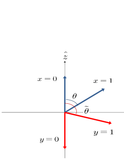
Figure 1: (Color online) The schematic diagram for measurement axis of Alice and Bob.

3.2 Physical situations

Our purpose is to study the possibility of making the hypothetical correlations of the PR box between Alice and Bob by quantum states with the modified quantum probability rule for Bob’s measurement. Now suppose that the following entangled state is shared between Alice and Bob,

$$|\psi\rangle_{AB}=\alpha|\uparrow\rangle_{A}|\downarrow\rangle_{B}+\beta|\downarrow\rangle_{A}|\uparrow\rangle_{B},~{}~{}~{}|\alpha|^{2}+|\beta|^{2}=1,$$ (3)

where subscripts $A$ and $B$ represent Alice and Bob respectively as before. $|\updownarrow\rangle$ are eigenstates of Pauli operator $\sigma_{z}$. Suppose the outcomes of $|\uparrow\rangle$ and $|\downarrow\rangle$ are $0$ and $1$ respectively for $\sigma_{z}$ measurement to use the same notation as the outputs of the PR box. Alice and Bob each have two different axis of measurement such as in Fig. 1, where the arrowhead represents the measurement direction which gives outcome $0$. The outcome corresponding to the opposite direction is $1$. Where the angle $\theta$ is measured from the positive $z$-axis to the positive $x$-axis. Alice measures along one of two directions $z$ and $\theta$ which correspond to one of two inputs $x=0$ and $x=1$. The relations between eigenstates of $\sigma_{z}$ and $\sigma_{\theta}$ are as follows

$$|\uparrow\rangle_{A}=\cos{\frac{\theta}{2}}|\theta\rangle_{A}+\sin{\frac{\theta}{2}}|\theta_{\perp}\rangle_{A},~{}~{}|\downarrow\rangle_{A}=-\sin{\frac{\theta}{2}}|\theta\rangle_{A}+\cos{\frac{\theta}{2}}|\theta_{\perp}\rangle_{A}.$$ (4)

Where $|\theta\rangle$ and $|\theta_{\perp}\rangle$ are two orthonormal eigenstates of $\sigma_{\theta}$ corresponding to outcomes $0$ and $1$ respectively. Bob takes measurements along either $-z$ ($y=0$) or $\tilde{\theta}$ ($y=1$) directions. Then relationships similar to Eq. (4) hold between eigenstates $\{|\uparrow\rangle_{B},|\downarrow\rangle_{B}\}$ and $\{|\tilde{\theta}\rangle_{B},|\tilde{\theta}_{\perp}\rangle_{B}\}$. We will explain calculations of $P(a,b|x,y)$ for the initial state $|\psi\rangle_{AB}$ with some typical inputs and outcomes under the ’modified quantum probability rule’ for Bob’s measurement and summarize all results.

We assume Alice and Bob are not moving relative to each other in order not to make any complexity related to simultaneity. Under our proposition the measurement of Alice is taken first and the quantum probability rule for Alice is governed by the usual Born rule. After the measurement of Alice the projected state becomes the pure separable state and so Bob’s measurement is taken on the pure state in his two-dimensional Hilbert space. The probability of Bob’s measurement will follow the modified quantum probability rule.

3.3 Calculations for the joint probabilities

Let us first consider a calculation of $P(0,0|0,0)$. In our case the $P(0,0|0,0)$ is calculated by the probability of outcome $b=0$ in Bob’s $y=0$ measurement under the condition that Alice’s outcome $a=0$ is given in her $x=0$ measurement. The outcome $a=0$ for $x=0$ is given only by $\alpha|\uparrow\rangle_{A}|\downarrow\rangle_{B}$ term of the initial state in Eq. (3). The projection probability from the initial state to $|\uparrow\rangle_{A}|\downarrow\rangle_{B}$ state is $|\alpha|^{2}$ since this projection is taken by Alice’s measurement. After the measurement of Alice, Bob’s state projected onto the state $|\downarrow\rangle_{B}$ because of the entanglement. This state gives outcome $b=0$ for the measurement $y=0$ with probability $1$. Therefore $P(0,0|0,0)=|\alpha|^{2}$. For measurement axis $x=0$ and $y=0$ there are no new results related to the modified quantum probability rule for Bob’s measurement since the state of Bob after Alice’s measurement is not a superposition of two outcome states. That is, $f(a_{0})=1$ for $f(a_{1})=0$ and vice versa in Eq. (1).

Next consider $y=1$ case, for example, $P(0,0|0,1)$. For $a=0$ and $x=0$ the state of Bob is projected onto $|\downarrow\rangle_{B}$ with probability $|\alpha|^{2}$ as before. Since Bob will take the $y=1$ measurement, the state of Bob must be rewritten as

$$|\downarrow\rangle_{B}=-\sin{\frac{\tilde{\theta}}{2}}|\tilde{\theta}\rangle_{B}+\cos{\frac{\tilde{\theta}}{2}}|\tilde{\theta}_{\perp}\rangle_{B},$$ (5)

by using the eigenstates of the $y=1$ measurement, $|\tilde{\theta}\rangle_{B}$ and $|\tilde{\theta}_{\perp}\rangle_{B}$ corresponding to outcomes $0$ and $1$ respectively. The outcome probability will be obtained by our ’modified quantum probability rule’ such that the probability of outcome $b=0$ for $y=1$ measurement will be $F_{0}(-\sin{\frac{\tilde{\theta}}{2}},\cos{\frac{\tilde{\theta}}{2}})$. Therefore

$$P(0,0|0,1)=|\alpha|^{2}F_{0}(-\sin{\frac{\tilde{\theta}}{2}},\cos{\frac{\tilde{\theta}}{2}}).$$ (6)

One of other nontrivial cases is $P(0,0|1,0)$. Here Bob’s measurement looks the same as that in the first case of $P(0,0|0,0)$, however, the nontriviality appears because of the different measurement of Alice. To get this joint probability Alice must take her measurement with $\sigma_{\theta}$ first. In this case the initial state must be rewritten by using the eigenstates of $x=1$ measurement such as

$$|\psi\rangle_{AB} = |\theta\rangle_{A}\left\{\alpha\cos{\frac{\theta}{2}}|\downarrow\rangle_{B}-\beta\sin{\frac{\theta}{2}}|\uparrow\rangle_{B}\right\}$$

$$+ |\theta_{\perp}\rangle_{A}\left\{\alpha\sin{\frac{\theta}{2}}|\downarrow\rangle_{B}+\beta\cos{\frac{\theta}{2}}|\uparrow\rangle_{B}\right\}.$$

Then the probability of outcome $a=0$ for $x=1$ is $|\alpha\cos{\frac{\theta}{2}}|^{2}+|\beta\sin{\frac{\theta}{2}}|^{2}$ according to the Born rule. After the measurement of Alice the state of Bob is projected onto the following normalized state,

$$\frac{1}{\sqrt{|\alpha|^{2}\cos^{2}{\frac{\theta}{2}}+|\beta|^{2}\sin^{2}{\frac{\theta}{2}}}}\left\{\alpha\cos{\frac{\theta}{2}}|\downarrow\rangle_{B}-\beta\sin{\frac{\theta}{2}}|\uparrow\rangle_{B}\right\}.$$ (8)

The probability of outcome $b=0$ for $y=0$ measurement will be $F_{0}(\alpha\cos{\frac{\theta}{2}},-\beta\sin{\frac{\theta}{2}})$ according to the modified quantum probability rule. Therefore the result becomes

$$P(0,0|1,0)=\left(\left|\alpha\cos{\frac{\theta}{2}}\right|^{2}+\left|\beta\sin{\frac{\theta}{2}}\right|^{2}\right)F_{0}(\alpha\cos{\frac{\theta}{2}},-\beta\sin{\frac{\theta}{2}}).$$ (9)

Note that only local measurement of Bob follows our new quantum probability rule and the others are governed by the standard Born rule.

The summary of all results for the probability distributions $P(a,b|x,y)$ are as follows:
1. For $x=0$ and $y=0$ measurements,

$$P(0,0|0,0) = |\alpha|^{2},~{}~{}~{}~{}P(1,0|0,0)=0,$$ (10)

$$P(0,1|0,0) = 0,~{}~{}~{}~{}~{}~{}~{}P(1,1|0,0)=|\beta|^{2}.$$

The total probability $P(x=0;y=0)$ which is the sum of all possible outcomes for inputs $x=0$ and $y=0$, i.e., $P(0,0|0,0)+P(1,0|0,0)+P(0,1|0,0)+P(1,1|0,0)$ is $1$ as expected.
2. For $x=1$ and $y=0$ measurements,

$$P(0,0|1,0) = \mathcal{A}_{1}F_{0}(\alpha\cos{\frac{\theta}{2}},\beta\sin{\frac{\theta}{2}}),$$

$$P(1,0|1,0) = \mathcal{A}_{2}F_{0}(\alpha\sin{\frac{\theta}{2}},\beta\cos{\frac{\theta}{2}}),$$ (11)

$$P(0,1|1,0) = \mathcal{A}_{1}F_{0}(\beta\sin{\frac{\theta}{2}},\alpha\cos{\frac{\theta}{2}}),$$

$$P(1,1|1,0) = \mathcal{A}_{2}F_{0}(\beta\cos{\frac{\theta}{2}},\alpha\sin{\frac{\theta}{2}}),$$

where $\mathcal{A}_{1}\equiv|\alpha|^{2}\cos^{2}{\frac{\theta}{2}}+|\beta|^{2}\sin^{2}{\frac{\theta}{2}}$ and $\mathcal{A}_{2}\equiv|\alpha|^{2}\sin^{2}{\frac{\theta}{2}}+|\beta|^{2}\cos^{2}{\frac{\theta}{2}}$.
3. For $x=0$ and $y=1$ measurement,

$$P(0,0|0,1) = |\alpha|^{2}F_{0}(\sin{\frac{\tilde{\theta}}{2}},\cos{\frac{\tilde{\theta}}{2}})$$

$$P(1,0|0,1) = |\beta|^{2}F_{0}(\cos{\frac{\tilde{\theta}}{2}},\sin{\frac{\tilde{\theta}}{2}})$$ (12)

$$P(0,1|0,1) = |\alpha|^{2}F_{0}(\cos{\frac{\tilde{\theta}}{2}},\sin{\frac{\tilde{\theta}}{2}})$$

$$P(1,1|0,1) = |\beta|^{2}F_{0}(\sin{\frac{\tilde{\theta}}{2}},\cos{\frac{\tilde{\theta}}{2}}).$$

4. For $x=1$ and $y=1$ measurements,

$$P(0,0|1,1) = \mathcal{A}_{1}F_{0}(\mathcal{C}_{1},\mathcal{C}_{2}),$$

$$P(1,0|1,1) = \mathcal{A}_{2}F_{0}(\mathcal{D}_{1},\mathcal{D}_{2}),$$ (13)

$$P(0,1|1,1) = \mathcal{A}_{1}F_{0}(\mathcal{C}_{2},\mathcal{C}_{1}),$$

$$P(1,1|1,1) = \mathcal{A}_{2}F_{0}(\mathcal{D}_{2},\mathcal{D}_{1}),$$

where $\mathcal{C}_{1}\equiv\alpha\cos{\frac{\theta}{2}}\sin{\frac{\tilde{\theta}}{2}}+\beta\sin{\frac{\theta}{2}}\cos{\frac{\tilde{\theta}}{2}}$, $\mathcal{C}_{2}\equiv\alpha\cos{\frac{\theta}{2}}\cos{\frac{\tilde{\theta}}{2}}-\beta\sin{\frac{\theta}{2}}\sin{\frac{\tilde{\theta}}{2}}$, $\mathcal{D}_{1}\equiv-\alpha\sin{\frac{\theta}{2}}\sin{\frac{\tilde{\theta}}{2}}+\beta\cos{\frac{\theta}{2}}\cos{\frac{\tilde{\theta}}{2}}$, and $\mathcal{D}_{2}\equiv\alpha\sin{\frac{\theta}{2}}\cos{\frac{\tilde{\theta}}{2}}+\beta\cos{\frac{\theta}{2}}\sin{\frac{\tilde{\theta}}{2}}$. Here only $F_{0}$ appears since we can represent $F_{1}(p,q)$ by $F_{0}(q,p)$ using bases relabeling invariance.

We will study constraints on the functional form of modified quantum probability $F_{0}(\alpha_{0},\alpha_{1})$ in Eq. (1) under the no-signaling condition. The no-signaling condition between Alice and Bob requires that an outcome of Bob’s measurement must not depend on the choice of measurement axes of Alice. This condition is satisfied when $\sum_{a}P(a,b|x,y)=\sum_{a}P(a,b|\tilde{x},y)$ for all values of $b$ and $y$. Where $\tilde{x}$ is $1+x$ mod 2. As a specific example let us consider $b=0$ and $y=0$ case. In this case the no-signaling condition becomes $P(0,0|0,0)+P(1,0|0,0)=P(0,0|1,0)+P(1,0|1,0)$ which gives

$$|\alpha|^{2}$$

$$= \left(|\alpha|^{2}\cos^{2}{\frac{\theta}{2}}+|\beta|^{2}\sin^{2}{\frac{\theta}{2}}\right)F_{0}(\alpha\cos{\frac{\theta}{2}},\beta\sin{\frac{\theta}{2}})$$

$$+ \left(|\alpha|^{2}\sin^{2}{\frac{\theta}{2}}+|\beta|^{2}\cos^{2}{\frac{\theta}{2}}\right)F_{0}(\alpha\sin{\frac{\theta}{2}},\beta\cos{\frac{\theta}{2}})$$

The equality cannot be satisfied in general by arbitrary functions $F_{0}(p,q)$. Here $\theta$ is the angle of Alice’s measurement axis so that Alice can determine her $\theta$ arbitrarily. The theory which restricts on the measurement axis cannot be considered as a proper physical theory. There are two kinds of solutions of Eq. (3.3) for arbitrary $\theta$. One is $|\alpha|=|\beta|$ which becomes the Bell state. The post-quantum theories must include other states than the Bell state because of the symmetry of a Hilbert space. A unitary evolution corresponding to a symmetry operation in a Hilbert space will change the Bell state to other state in general. Therefore this solution cannot give a full physical theory. Another kind can be found by setting $\theta=\pi/2$, then the functional form of $F_{0}(x,y)$ are determined such as

$$|\alpha|^{2}=F_{0}(\frac{\alpha}{\sqrt{2}},\frac{\beta}{\sqrt{2}}).$$ (15)

Considering the state normalization condition this implies $F_{0}(\alpha,\beta)=|\alpha|^{2}$ which is the Born rule. This implies even the minimal modification of the quantum probability rule only for Bob is restricted by no-signaling condition. Therefore, we conclude that we cannot make a post-quantum theory by the modification of the quantum probability rule from the Born rule without violating no-signaling principle.

3.4 Simulating the PR boxes

It is still interesting, however, to consider whether the PR box can be simulated by our model since the concrete mechanism for generating non-local boxes including the PR box is lack except the linear combinations or wiring of two nonlocal boxes [11].

To simulate the non-local boxes we use the following explicit functional form for the probability assignment

$$F_{0}(\alpha_{0},\alpha_{1})=\frac{|\alpha_{0}|^{n}}{|\alpha_{0}|^{n}+|\alpha_{1}|^{n}}.$$ (16)

When the initial state $|\psi\rangle_{AB}$ in Eq. (3) is the Bell state, i.e., for $|\alpha|=|\beta|=1/\sqrt{2}$ the probability distributions $P(a,b|x,y)$ become

$$P(0,0|0,0) = P(1,1|0,0)=\frac{1}{2},$$ (17)

$$P(1,0|0,0) = P(0,1|0,0)=0,$$

$$P(0,0|1,0) = P(1,1|1,0)=\frac{1}{2}\frac{|\cos{\frac{\theta}{2}}|^{n}}{|\cos{\frac{\theta}{2}}|^{n}+|\sin{\frac{\theta}{2}}|^{n}},$$

$$P(1,0|1,0) = P(0,1|1,0)=\frac{1}{2}\frac{|\sin{\frac{\theta}{2}}|^{n}}{|\cos{\frac{\theta}{2}}|^{n}+|\sin{\frac{\theta}{2}}|^{n}},$$

$$P(0,0|0,1) = P(1,1|0,1)=\frac{1}{2}\frac{|\sin{\frac{\tilde{\theta}}{2}}|^{n}}{|\cos{\frac{\tilde{\theta}}{2}}|^{n}+|\sin{\frac{\tilde{\theta}}{2}}|^{n}},$$

$$P(1,0|0,1) = P(0,1|0,1)=\frac{1}{2}\frac{|\cos{\frac{\tilde{\theta}}{2}}|^{n}}{|\cos{\frac{\tilde{\theta}}{2}}|^{n}+|\sin{\frac{\tilde{\theta}}{2}}|^{n}},$$

$$P(0,0|1,1) = P(1,1|1,1)=\frac{1}{2}\frac{|\sin{\frac{\theta+\tilde{\theta}}{2}}|^{n}}{|\sin{\frac{\theta+\tilde{\theta}}{2}}|^{n}+|\cos{\frac{\theta+\tilde{\theta}}{2}}|^{n}}$$

$$P(1,0|1,1) = P(0,1|1,1)=\frac{1}{2}\frac{|\cos{\frac{\theta+\tilde{\theta}}{2}}|^{n}}{|\sin{\frac{\theta+\tilde{\theta}}{2}}|^{n}+|\cos{\frac{\theta+\tilde{\theta}}{2}}|^{n}}$$

One can easily check that the no-signaling condition is satisfied for arbitrary $\theta$, $\tilde{\theta}$, and $n$. This implies that there is no restriction on the measurement angle for the Bell state. The condition that the above probability distributions reproduce the probability distributions of the PR Box requires, in the limit of $n\rightarrow\infty$,

$$\Big{|}\cos{\frac{\theta}{2}}\Big{|}>\Big{|}\sin{\frac{\theta}{2}}\Big{|},~{}~{}~{}\Big{|}\sin{\frac{\tilde{\theta}}{2}}\Big{|}>\Big{|}\cos{\frac{\tilde{\theta}}{2}}\Big{|}$$ (18)

and $$\Big{|}\cos{\frac{\theta+\tilde{\theta}}{2}}\Big{|}>\Big{|}\sin{\frac{\theta+\tilde{\theta}}{2}}\Big{|}.$$

To satisfy the above requirements, the angle $\theta$ must be either in the first or the fourth quadrant and the angle $\tilde{\theta}$ either in the second or the third quadrant. Additionally, the angles $\theta$ and $\tilde{\theta}$ also have to satisfy one of $0<\theta+\tilde{\theta}<\frac{\pi}{2}$, $\frac{3\pi}{2}<\theta+\tilde{\theta}<\frac{5\pi}{2}$ and $\frac{7\pi}{2}<\theta+\tilde{\theta}<4\pi$. There is always a suitable $\tilde{\theta}$ for any $\theta$ to satisfy one of those conditions. For these angles the probabilities go to $1/2$ for inputs and outcomes which satisfy $a\oplus b=xy$ and zeros for others in the limit of $n\rightarrow\infty$. These probability distributions are the same as those of the PR box. Therefore the PR box can be simulated by the Bell states with the modified quantum probability rule in Eq. (16) for $n=\infty$.

4 Other nonlocal boxes

The joint probability distributions in Eq. (17) are continuous functions of the angles $\theta$, $\tilde{\theta}$ and the power $n$ under the modified quantum probability rule Eq. (16), therefore, they will describe other nonlocal boxes for other $\theta$, $\tilde{\theta}$ and $n$. The joint probability distributions in our model is obtained by the modified quantum probability rule for the quantum measurement so that different observable sets described by $\theta$ and $\tilde{\theta}$ could generate other joint probability distributions also depending on the power $n$ of the modified Born rule. In this way we can get a variety of nonlocal correlations which generate nonlocal boxes. Another interesting example is the nonlocal box (NLB) which can be generated by the observables in the standard CHSH inequality [2]. We will study the nonlocality of these nonlocal boxes in this section.

4.1 CHSH nonlocality for our non-isotropic NLBs

First we will study the nonlocality of the non-isotropic NLBs which is described by the joint probability distributions in Eq. (17). We will explain what means the non-isotropic boxes later. We will use the CHSH nonlocality [22] to measure the nonlocality of our non-isotropic NLBs.

The CHSH nonlocality of our nonlocal boxes $P_{NL}$ is defined by the value

$$\mathcal{B}(P_{NL})=\max_{xy}|C_{xy}(P_{NL})+C_{x\tilde{y}}(P_{NL})+C_{\tilde{x}y}(P_{NL})-C_{\tilde{x}\tilde{y}}(P_{NL})|,$$ (19)

where $x$ and $y$ are two binary inputs and $\tilde{x}=x+1$ and $\tilde{y}=y+1$ modulo $2$ as before. The $C_{xy}$ is the correlation function defined as

$$C_{xy}(P_{NL})=P(0,0|x,y)+P(1,1|x,y)-P(0,1|x,y)-P(1,0|x,y).$$ (20)

To find out the specific inputs $x$ and $y$ which give the maximum value for the CHSH value $\mathcal{B}(P_{NL})$ we use the continuity of the joint probability functions with respect to the power $n$. When $n$ goes to infinity, the joint probability distributions becomes those for the PR box which give the CHSH value 4. This corresponds to $C_{11}(P_{NL})\rightarrow-1$ for $n\rightarrow\infty$ so $\tilde{x}$ and $\tilde{y}$ must be 1. That is, $x$ and $y$ are $0$.

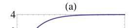
Figure 2: (Color online) (a) This shows the dependence of the CHSH value $\mathcal{B}(P_{NL}$ on the power $n$. (b) This shows the dependence of $CHSH(P)$ on $\tilde{\theta}$ for $n=10$ and two different $\theta$ values, $\frac{3\pi}{8}$ and $\frac{\pi}{4}$.

Therefore the CHSH value of our non-isotropic NLBs for arbitrary $n$ becomes

$$\mathcal{B}(P_{NL}) = 1+g_{0}(\sin{\frac{\tilde{\theta}}{2}},\cos{\frac{\tilde{\theta}}{2}})-g_{1}(\sin{\frac{\tilde{\theta}}{2}},\cos{\frac{\tilde{\theta}}{2}})+g_{1}(\sin{\frac{{\theta}}{2}},\cos{\frac{{\theta}}{2}})$$

$$- g_{0}(\sin{\frac{{\theta}}{2}},\cos{\frac{{\theta}}{2}})+g_{1}(\sin{\frac{\theta+\tilde{\theta}}{2}},\cos{\frac{\theta+\tilde{\theta}}{2}})-g_{0}(\sin{\frac{\theta+\tilde{\theta}}{2}},\cos{\frac{\theta+\tilde{\theta}}{2}}),$$

where $g_{0}(\alpha_{0},\alpha_{1})=|\alpha_{0}|^{n}/(|\alpha_{0}|^{n}+|\alpha_{1}|^{n})$ and $g_{1}(\alpha_{0},\alpha_{1})=|\alpha_{1}|^{n}/(|\alpha_{0}|^{n}+|\alpha_{1}|^{n})$ The results are shown in the Fig. 2. Fig. 2 (a) shows a monotonic increasing behavior of the CHSH value $\mathcal{B}(P_{NL})$ for the power $n$. The angles of measurement axes $\theta$ and $\tilde{\theta}$ satisfy the condition to simulate the PR box. In this figure $\theta=\pi/4$ and $\tilde{\theta}=11\pi/8$. Fig 2 (b) shows the angle $\tilde{\theta}$ dependence of the CHSH value for $n=20$ which is large enough for the CHSH value to saturate to its maximum value. The real line and dashed line corresponds to $\theta=3\pi/8$ and $\theta=\pi/4$ respectively. There are two kinds of change in the graphs. The first kind of change occurs at different values of $\tilde{\theta}$. This kind of change occurs first in the real line and is followed by the dashed line. This is because $\theta+\tilde{\theta}$ of the real line is greater than that of the dashed line. The $\theta+\tilde{\theta}$ determines the probability distributions for $x=1$ and $y=1$ as one can see in Eq. (17). The second kind of change start at the same point, i.e., $\tilde{\theta}=\pi/2$ and $\tilde{\theta}=3\pi/2$. These values are related with the condition $\tilde{\theta}$ must be either in the second or the third quadrant, $\pi/2<\tilde{\theta}<3\pi/2$ for the CHSH value to be the maximum value for $n\rightarrow\infty$.

These results imply that the application of the modified quantum probability rule provide the systematic way of obtaining new nonlocal boxes. These nonlocal boxes are not isotropic since the correlation functions does not satisfy the condition for the unbiased marginal distributions [23]

$$C_{00}=C_{01}=C_{10}=-C_{11}.$$ (22)

The properties of nonlocality such as information causality [12] and computational complexity [10] et al. are studied by the nonlocal boxes so the discovery of the systematic way to obtain new nonlocal boxes is very important.

4.2 Nonlocal boxes defined by the CHSH observables

The joint probability distributions in our model depend not only on the state and the probability rule but the observables. It is interesting to consider the standard CHSH observables and the CHSH inequality for the modified quantum probability rule. The CHSH parameter $\mathcal{B}$ defined as

$$\mathcal{B}=\langle\mathcal{Q}\mathcal{S}\rangle+\langle\mathcal{R}\mathcal{S}\rangle+\langle\mathcal{R}\mathcal{T}\rangle-\langle\mathcal{Q}\mathcal{T}\rangle.$$ (23)

Where $\mathcal{Q}=\sigma_{z}^{A}$, $\mathcal{S}=-(\sigma_{z}^{B}+\sigma_{x}^{B})/\sqrt{2}$, $R=\sigma_{x}^{A}$, and $T=(\sigma_{z}^{B}-\sigma_{x}^{B})/\sqrt{2}$ are the CHSH observables. The superscripts $A$ and $B$ represent Alice and Bob respectively. And $\sigma_{i}$’s are Pauli matrices. In our case Alice measures first before Bob’s measurement. An expectation value $\langle\mathcal{Q}\mathcal{S}\rangle$ is a quantum correlation of two observables $\mathcal{Q}$ and $\mathcal{S}$. Since observables have eigenvalues $\pm 1$, the expectation value $\langle\mathcal{Q}\mathcal{S}\rangle$ is calculated as follows

$$\langle\mathcal{Q}\mathcal{S}\rangle = 1\times P(1_{\mathcal{Q}})\left\{1\times P(1_{\mathcal{S}}|1_{\mathcal{Q}})+(-1)\times P(-1_{\mathcal{S}}|1_{\mathcal{Q}})\right\}$$

$$+ (-1)\times P(-1_{\mathcal{Q}})\left\{1\times P(1_{\mathcal{S}}|-1_{\mathcal{Q}})+(-1)\times P(-1_{\mathcal{S}}|-1_{\mathcal{Q}})\right\}.$$

$P(\pm 1_{\mathcal{Q}})$ are probabilities to obtain eigenvalues $\pm 1$ respectively for the observable $\mathcal{Q}$. To calculate $P(\pm 1_{\mathcal{Q}})$ the initial state must be expanded by using the eigenstates of the observable $\mathcal{Q}$. The probability of outcomes $\pm 1$ for observables $\mathcal{Q}$ and $\mathcal{R}$ of Alice are determined by the Born rule in our model. After the projective measurement of Alice the state of Bob will be projected to the pure state in the two-dimensional Hilbert space in which the probability for Bob’s measurement is determined by the modified quantum probability rule. For example the $P(\pm 1_{\mathcal{S}}|\pm 1_{\mathcal{Q}})$ are the conditional probability calculated by using modified quantum probability rule for the observable $\mathcal{S}$ on the projected state of Bob after projective measurement of Alice by the observable $\mathcal{Q}$.

We can define the nonlocal boxes by the CHSH observables with the modified Born rule. Let these nonlocal boxes be $P_{CHSH}(n)$, where $n$ represents the dependence on the power of the modified Born rule. The binary inputs $x=0$ and $x=1$ of $P_{CHSH}(n)$ correspond to the measurements by $R$ and $Q$ respectively and $y=0$ and $y=1$ to the measurements by $T$ and $S$ respectively. Then $\langle RT\rangle$ becomes the same as the correlation function $C_{00}(P_{CHSH}(n))$ defined in Eq. (20). As a result the CHSH parameter $\mathcal{B}$ also becomes the same as the CHSH value $\mathcal{B}(P_{CHSH}(n))$. These nonlocal boxes $P_{CHSH}(n)$ are isotropic nonlocal boxes which satisfy the condition of the unbiased marginal distributions Eq. (22).

The CHSH parameter is calculated as

$$\mathcal{B}=4\frac{\sqrt{2+\sqrt{2}}^{n}-\sqrt{2-\sqrt{2}}^{n}}{\sqrt{2+\sqrt{2}}^{n}+\sqrt{2-\sqrt{2}}^{n}}$$ (25)

Fig. 3 shows the dependence of the CHSH parameter $\mathcal{B}$ on the power $n$. When $n$ changes from zero to infinity, the CHSH $\mathcal{B}$ covers all values up to $4$. Therefore the Bell state with the modified quantum probability in Eq. (16) for arbitrary $n$ can simulate nonlocal boxes with all CHSH $\mathcal{B}$ higher than the quantum upper bound. When $n$ goes to infinity the CHSH parameter becomes the maximum value $4$ as expected for the PR box. The $\mathcal{B}$ goes to the approximate value $4$ very rapidly so that $\mathcal{B}$ becomes approximately 3.999 for $n=10$. According to Brassard et al. [7], the isotropic nonlocal boxes with $\mathcal{B}$ more than $4\sqrt{2/3}$ makes communication complexity trivial. This value $4\sqrt{2/3}$ is achieved for $n\approx 2.601$.

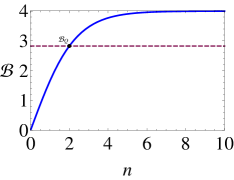
Figure 3: (Color online) The CHSH parameter $\mathcal{B}$ versus power $n$ of the modified Born rule of Bob. It shows $\mathcal{B}$ approaches quickly to $4$ with increasing $n$. The dot represent the quantum Tsirelson’s bound $2\sqrt{2}$. The point $\mathcal{B}_{Q}$ represents the $\mathcal{B}$ for the Born rule of Bob.

5 Discussions and Summary

The theory to make communication complexity trivial is strongly believed not to exist [11]. There was, however, no concrete reason for this belief. In this paper we have studied the possibility of the post-quantum theory candidates by applying the modified quantum probability rule for the second party under the local measurement requirements. The measurement of second party is always on the projected pure separable state so the modification of the quantum probability rule is minimal. This minimal modification of the quantum probability gives the post-quantum theory candidates which could have the nonlocality greater than that of the quantum theory. These post-quantum theory candidates, however, cannot be consistent with the symmetry of the Hilbert space which requires the freedom on the angle of measurement axis. In the post-quantum theory candidates the measurement angle for an arbitrary entangled state is restricted under the no-signaling condition. In a linear quantum mechanics Hilbert space description is natural so that we believe the only possible extension of the quantum mechanics comes from the measurement postulates, especially, the quantum probability rule. Therefore our study suggests that there is no physical theories other than the quantum theory under the condition of the no-signaling principle and the local measurement requirements. The theory with $n\leq 2$ is not our concern since the nonlocality of those theories are covered by quantum mechanics. Moreover, the nonlinear extensions of quantum mechanics proposed by Weinberg [24] might be used to send superluminal signals [24, 25, 26]. This reinforce our belief that there are no other physical theories than the quantum mechanics under the condition of no-signaling principle and local measurements. Therefore this could be a partial explanation for why the nonlocality of the quantum theory is limited.

In summary, we have studied the effect of the modified quantum probability rule for the quantum measurement on the nonlocality. The nonlocal quantum correlation manifests itself by correlations of measurement outcomes. Therefore the modification of the quantum probability rule for the measurement changes nonlocality between two spacelike separate parties. The change of nonlocality was represented by the joint probability distributions. The joint probability distributions, however, must be given by the Born rule when the no-signaling condition and the freedom of choice of measurement axes are required. Other quantum postulates than the quantum measurement postulates are about Hilbert space which is hard to modify within physically reasonable bound. We have shown that the probability distributions of the PR box can be approximately simulated by our model using explicit function of the modified quantum probability. When the power of quantum probability goes to infinity for proper values of the measurement angles, the probability distributions of the PR box is reproduced by the Bell state. We have shown that for the other value of the power and measurement angles the Bell state can simulate various nonlocal boxes. We have found the probability distributions for the anisotropic nonlocal boxes with the CHSH values up to 4. We have shown the CHSH observables in the usual CHSH inequality generate the isotropic nonlocal boxes with the CHSH values up to 4. This implies that our model can be used as a systematic way to obtain various nonlocal boxes. The nonlocal boxes with quantum theory-like property will help to understand the non-locality related properties such as communication complexity and information causality more deeply.

References

References

- [1] Bell J S 1964 Physics 1 195
- [2] Clauser J F, Horne M A, Shimony A, and Holt R A 1969 Phys. Rev. Lett. 23 880
- [3] Tsirelson B S 1980 Lett. Math. Phys. 4 93
- [4] S. Popescu and D. Rohrlich, Found. Phys. 24, 379 (1994).
- [5] Cleve R, Dam W van, Nielson M, and Tapp A 1999 Quantum Computing and Quantum Communication, Lecture Notes in Computer Science vol 1509 (Springer-Verlag)
- [6] Barrett J, Linden N, Massar S, Pironio S, Popescu S, and Roberts D 2005 Phys. Rev. A 71 022101
- [7] Brassard G, Buhrman H, Linden N, Methot A A, Tapp A, and Unger F 2006 Phys. Rev. Lett. 96 250401
- [8] Linden N, Popescu S, Short A J, and Winter A 2007 Phys. Rev. Lett. 99 180502
-
[9]
Navascués M, Pironio S and Acín A 2007 Phys. Rev. Lett. 98 010401
Navascués M, Pironio S and Acín A 2008 New J. Phys. 10 073013 - [10] Skrzypczyk P, Brunner N, and Popescu S 2009 Phys. Rev. Lett. 102 110402
- [11] Brunner N and Skrzypczyk P 2009 Phys. Rev. Lett. 102 160403
- [12] Pawlowski, Paterek T, Kazlikowski D, Scarani V, Winter A, and Zukowski M 2009 Nature 461 1101.
- [13] Cavalcanti D, Salles A, and Scarani V 2010 Nat. Commun. 1 136
- [14] Gallego R, Wurflinger L E, Acin A, and Navascues M 2011 Phys. Rev. Lett. 107 210403
- [15] Yang T H, Cavalcanti D, Almeida M L, Teo C, and Scarani V 2012 New J. Phys. 14 013061
- [16] Dahlsten Oscar C O, Lercher D, and Renner R 2012 New J. Phys. 14 063024
- [17] Weinberg S 1995 Quantum Theory of Fields vol 1 (Cambridge University Press)
- [18] Sorkin R D 1994 Mod. Phys. Lett. A 9 3119
- [19] Ududec C, Barnum H, and Emerson J 2011 Found. Phys. 41 396
- [20] Sinha U, Couteau C, Jennewein T, Laflamme R and Weihs G 2010 Science 329 418
- [21] Gleason A M 1957 J. Math. Mech. 6 885
- [22] Forster M, Winkler S, and Wolf S 2009 Phys. Rev. Lett. 102 120401
- [23] Masanes Ll, Acin A, and Gisin N 2006 Phys. Rev. A 73 012112
- [24] Weinberg S 1989 Ann. Phys. (N. Y.) 194 336; 1989 Phys. Rev. Lett. 62 485
- [25] Gisin N 1989 Helv. Phys. Acta 62 363; 1990 Phys. Lett. A 143 1
- [26] Polchinski J 1991 Phys. Rev. Lett. 66 397