Characterizing flows with an instrumented particle measuring Lagrangian accelerations

Abstract

We present in this article a novel Lagrangian measurement technique: an instrumented particle which continuously transmits the force/acceleration acting on it as it is advected in a flow. We develop signal processing methods to extract information on the flow from the acceleration signal transmitted by the particle. Notably, we are able to characterize the force acting on the particle and to identify the presence of a permanent large-scale vortex structure. Our technique provides a fast, robust and efficient tool to characterize flows, and it is particularly suited to obtain Lagrangian statistics along long trajectories or in cases where optical measurement techniques are not or hardly applicable.

Turbulence is omnipresent in nature and in industry, and has received much attention for years. In the specific field of experimental fluid dynamics research, very significant progress has been achieved during the last decade with the advent of space and time resolved optical techniques based on high speed imaging Tropea et al. (2007). However, a direct resolution of the Eulerian flow pattern is still not always possible nor simple to carry out. In this context, Lagrangian techniques, in which the fields are monitored along the trajectories of particles, provide an interesting alternative Toschi and Bodenschatz (2009); Shraiman and Siggia (2000) with information about the small scales of turbulence (especially isotropy) and a huge focus on the particle’s Lagrangian acceleration that directly reflects the turbulent forces exerted on the particles Voth et al. (2002); Mordant et al. (2003); Qureshi et al. (2007, 2008); Volk et al. (2008); Xu and Bodenschatz (2008).

From an experimental point of view several inconveniences arise. In the Lagrangian frame one would like to collect long trajectories. However, even in confined flows it is difficult to track even just a few particles over a long time using the existing methods. For instance to use optical methods, the flow must be entirely observed and continuously recorded, something which is not yet possible. Apart from its implication for computing converged statistical quantities, several theories such as the fluctuation theorem necessitate long trajectories instead of many short ones. Another issue is the possible rotation of large particles in a flow, and the influence of this possible rotation on the dynamics of the particle. An optical technique following simultaneously particle position and absolute orientation in time has been recently developed Zimmermann et al. (2011a). It shows in particular that for increasing turbulence, solid particles experience stronger rotation Zimmermann (2012); Zimmermann et al. (2011b). The technique used in those experiments is not straightforward and needs careful calibration and synchronization, as well as an expensive set-up (high-speed cameras, strong illumination, etc) as well as time-consuming post-processing. Other common Lagrangian techniques, e.g. particle tracking velocimetry (PTV), generally do not allow a direct measurement of the possible rotation of the particle simultaneously with its translation.

The experimental technique presented here was designed to overcome these issues thanks to the design of instrumented particles Gasteuil et al. (2007); Gasteuil (2009); Shew et al. (2007); Pinton et al. (2009). This was initially developed by our group to study Lagrangian particles with a temperature sensitive dependance, there used in Rayleigh-Bénard convection Ni et al. (2012). The approach is to instrument a neutrally buoyant particle in such a way that it measures the temperature as it is entrained by the flow, and to transmit the data via a radio frequency link to the lab operator. This way, one gains access to trajectories for as long as the particle’s battery lifetime. In the work reported here, we built upon this approach to instrument the particle with a 3D accelerometer such that one gets the accelerations – i.e. the forces – acting on a spherical particle in real time and for long trajectories. The instrumented particle has been previously tested, benchmarked and validated with the optical technique of Zimmermann et al. Zimmermann et al. (2012), showing a good agreement between the two different measurements of the acceleration. In the present work we establish methods to extract physical characteristics of the investigated flows from the particle’s acceleration signal.

One further motivation is to gain insights into a flow when direct imaging is not possible, e.g. when dealing with opaque vessels, non-transparent fluids or granular media. These constraints occur especially in industry where additional bio-medical or environmental constraints arise (the injection of tracer particles might be unsuitable and thus prevent any visualization technique). As mentioned above solid particles are found to rotate when advected in a highly turbulent flow Zimmermann et al. (2011b). We show here that it is possible to build quantities depending or not on the particle’s rotation and we conclude about flow parameters that are directly accessible without any optical measurement.

The article is organized as follows: first, we present the experimental setup, as well as a brief reminder of the technical characteristics of the instrumented particle and the forces it measures (section I). Then, we present the new signal processing methods (section II). Finally, we discuss and conclude on this new measurement technique (section III).

I Experimental setup

I.1 Instrumented particle

The device described in the following is designed and built by smartINST S.A.S., a spin-off from CNRS and the ENS de Lyon. It consists of an instrumented particle (the so-called smartPART ®), a spherical particle which embarks an autonomous circuit with 3D-acceleration sensor, a coin cell and a wireless transmission system, and a data acquisition center (the so-called smartCENTER ®) which receives, decodes, processes and stores the signals from the smartPART (see Fig. 1 and Fig. 2). The smartPART measures the three dimensional acceleration vector $\bm{a}_{\text{SP}}$ acting on the particle in the flow. It is in good agreement with other techniques, details can be found in Ref. Zimmermann et al. (2012).

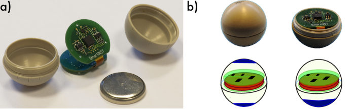
Figure 1: a) Picture of the instrumented particle (so-called smartPART from smartINST S.A.S.);  b) Possible mass distributions of the particle; its inertia consists mainly of a disk and a spherical shell, with different density adjustment and imbalance settings by adding Tungsten paste (in blue); experiments are best done with a symmetrical repartition of the masses.

The accelerometer consists of a micro-electro-mechanical system giving the three components of the acceleration (each of the three decoupled axes returns a voltage proportional to the force acting on a small mass-load suspended by micro-fabricated springs). From this construction arises a permanent measurement of the gravitational force/acceleration $\bm{g}\equiv 9.8\,\mathrm{m}/\mathrm{s}^{2}\cdot\bm{\hat{e}}_{z}=g\cdot\bm{\hat{e}}_{z}$. Each axis has a typical full-scale range of $\pm 3.6\,g=35\,\mathrm{m}/\mathrm{s}^{2}$. The sensor has to be calibrated in order to compute the physical accelerations from the voltages of the accelerometer. The detailed procedure is described in Ref. Zimmermann et al. (2012). Concerning the resolution of the smartPART, the uncertainty on the acceleration norm is $\left\lvert\bm{\sigma}\right\rvert=\sqrt{\sum_{i}\sigma_{i}^{2}}=0.008\,g$, with an average noise $\sigma_{i}\leq 0.005\,g$ on each axis.

The particle rotates freely and in an a priori unknown way as it is advected by the flow. The instantaneous orientation of the particle can be described by an absolute orientation with respect to a reference coordinate system, $\smash{\underline{\underline{\mathbf{R}}}}(t)$ Goldstein (2002). For readability we only write the time reference when necessary (e.g. when two different times are involved in an equation) and drop it otherwise. Using this rotation matrix, it is possible to express the contributions to the force acting on the particle and measured by the acceleration sensor in the lab frame or in the particle frame. The following contributions to the particle’s acceleration signal $\bm{a}_{\text{SP}}$ can be identified:

(i) Gravity:

By construction, gravity $\bm{g}$ is always contributing to $\bm{a}_{\text{SP}}$. Since the particle is a priori oriented arbitrarily in space, $\bm{g}$ is projected onto all 3 axes.

(ii) Translation:

The forces acting on the particle are projected as the Lagrangian acceleration $\displaystyle{\bm{\bm{a}_{\text{trans}}}=\frac{\text{d}^{2}}{\text{d}t^{2}}\bm{x}(t)}$ onto the sensor.

(iii) Rotation:

The particle rotates freely around its geometrical center with an angular velocity $\bm{\omega}$. If the sensor is placed by $\bm{r}$ outside the geometrical center of the sphere one observes the centrifugal force: $\displaystyle{\bm{a}_{\text{cf}}=\bm{\omega}\times\left(\bm{\omega}\times\bm{r}\right)+\left(\frac{\text{d}}{\text{d}t}\bm{\omega}\right)\times\bm{r}}$. According to the technical drawings it is $\bm{r}\approx 3\;\mathrm{m}\mathrm{m}\cdot\hat{e}_{z}$. Experiments on the rotation of the smartPART in a von Kármán flow created by two counter-rotating impellers show that the angular velocity $\omega$ of the particle is of the order of the impeller frequency $f_{\text{imp}}$ Zimmermann et al. (2011b); Zimmermann et al. (2012). The rotational forces are of order $\displaystyle{r\,\omega^{2}\sim{r}\cdot({4\pi^{2}\,f_{\text{imp}}^{2}})\lesssim 0.1\,\left\lvert\bm{a}_{\text{trans}}\right\rvert}$ and have consequently negligible effect. A more detailed analysis measured that the ratio between the contribution due to the rotation and the total acceleration is $\displaystyle{{\left\lvert\bm{a}_{\text{cf}}\right\rvert}/{\left\lvert\bm{a}_{\text{trans}}+\bm{a}_{\text{cf}}\right\rvert}<0.1}$ Zimmermann et al. (2012). The contribution due to the rotation is thus neglected. It has to be noted that by construction of the accelerometer and because the circuit is fixed within the sphere, there is no contribution of the Coriolis force.

(iv) Noise & spikes:

In ideal situations the smartPART has a noise of less than $0.005\,g$ for each axis, which can be handled by a moving average. Wrong detections appear as strong deviations from the signal and are hard to distinguish from high acceleration events due to the turbulent flow or contacts with e.g. the impellers. Experiments in different configurations prove the remaining noise to be negligible Zimmermann et al. (2012).

Combining the different terms, and neglecting possible noise and the rotational bias yields:

$$\begin{split}\bm{a}_{\text{SP}}&\approx\,\smash{\underline{\underline{\mathbf{R}}}}\,\left[\bm{g}+\frac{\text{d}^{2}\;}{\text{d}t^{2}}\bm{x}\right]=\smash{\underline{\underline{\mathbf{R}}}}\,\left[\bm{g}+\bm{a}_{\text{trans}}\right].\end{split}$$ (1)

The contributions due to gravity and translation are thus entangled by the continuously changing orientation of the particle. Since gravity is of little interest here, one has to investigate how common quantities such as the mean and the variance (or rms) of the acceleration time series as well as auto correlation functions can give information about the particle motion.

Considering robustness, the smartPART is able to continuously transmit data for a few days. During various experiments in a von Kármán flow neither contacts with the wall nor with the sharp edged blades of the fast rotating impellers damaged its function or shell. Furthermore, the sensor has among other things been chosen for its weak temperature dependance; in order to achieve optimal precision of the measurements, we calibrate the particle at experiment temperature shortly before the actual experiment.

Finally, by adding Tungsten paste to the inside of the smartPART the weight of the particle can be adjusted such that the particle is neutrally buoyant in de-ionized water at $20\,\degreecelsius$. It should be noted that the mass distribution inside the particle is neither homogeneous nor isotropic. The particle’s inertia is best described by a heavy disk of $20\;\mathrm{m}\mathrm{m}$ diameter (the battery), a spherical shell and patches of Tungsten paste. The paste must, therefore, be added carefully to minimize the imbalance of the particle (see Fig. 1b); otherwise the resulting out-of-balance particle (i.e. with the center of mass not coinciding with the geometrical center) induces a strong preferential orientation and wobbles similar to a kicked physical pendulum. For a well balanced particle, which rotates easily in the flow, one of the eigen-axes of inertia then coincides (approximately) with the $z-$axis of the accelerometer. The other two are within the $x-y$ plane due to rotational symmetry.

I.2 Von Kármán swirling flow

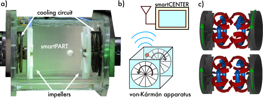
Figure 2: a) Picture of the von Kármán swirling flow with the instrumented particle inside;  b) Sketch of the experimental setup with the apparatus and the smartPART transmitting acceleration signals to the smartCENTER;  c) Sketch of the global structures that can be found with the two co- and counter-rotating regimes.

We investigate the motion of the instrumented particle in a fully turbulent flow. Namely, we use a von Kármán swirling flow; in contrast to Ref. Zimmermann et al. (2011b) the apparatus is here filled with water and develops higher turbulence rates. A swirling flow is created in a square tank by two opposing counter-rotating impellers of radius $R=9.5\,\mathrm{c}\mathrm{m}$ fitted with straight blades $1\,\mathrm{c}\mathrm{m}$ in height (see Fig. 2). The flow domain in between the impellers has characteristic length $H=20\,\mathrm{c}\mathrm{m}\cong 2R$. Blades on the impellers work similar to a centrifugal pump and add a poloidal circulation at each impeller. For counter-rotating impellers, this type of flow is known to exhibit fully developed turbulence Ravelet et al. (2008). Within a small region in the center the mean flow is little and the local characteristics approximate homogeneous turbulence. However, at large scales it is known to be anisotropic Ouellette et al. (2006); Monchaux et al. (2006). Key parameters of the turbulence at different impeller speeds are given in Table 1. The two impellers can also be driven co-rotating, creating a highly-turbulent flow inside the vessel with one pronounced persistent global vortex along the axis of rotation. Close to the axis of rotation the mean flow is weak, followed by a strong toroidal component and an additional poloidal circulation induced by blades on the impellers. The energy injection rate is a factor of 2 smaller than for counter-rotating impellers. This means that at the same impeller frequency, $f_{\text{imp}}$, co-rotating driving creates less turbulence than counter-rotation, but the flow is still highly turbulent Simand (2002). Although the vortical structures near the disks are comparable (see Fig. 2c), the co- or counter-rotating regimes yield well distinct global structures in the center of the vessel. The two regimes are used to compare the signals obtained by the instrumented particle in two very different flow configurations. In addition, the co-rotating serves as a test case for persistent, large vortex structures as they are found in mixers with only one impeller.

$f_{\text{imp}}[\mathrm{Hz}]$	$Re$	$R_{\lambda}$	$\varepsilon[\mathrm{m}\mathrm{{}^{2}}\mathrm{/}\mathrm{s}\mathrm{{}^{3}}]$	$\eta[\mathrm{\SIUnitSymbolMicro}\mathrm{m}]$	$\tau_{\eta}[\mathrm{m}\mathrm{s}]$	$T_{\text{int}}[\mathrm{s}]$
$1.0$	$62800$	$290$	$0.07$	$62$	$3.8$	$1.00$
$2.0$	$125700$	$410$	$0.48$	$38$	$1.4$	$0.50$
$3.0$	$188500$	$505$	$1.68$	$28$	$0.8$	$0.33$
$4.0$	$251300$	$580$	$4.03$	$22$	$0.5$	$0.25$

Table 1: Key-parameters of the counter-rotating flow configuration. The integral time scale is defined as $T_{\text{int}}=1/f_{\text{imp}}$ and the integral length scale is estimated to be $L_{\text{int}}=3\;\mathrm{c}\mathrm{m}$. We use the following definition for the Reynolds numbers: $Re=2\pi R^{2}f_{\text{imp}}/\nu$ and $R_{\lambda}\approx\sqrt{\frac{15}{\nu}\cdot 2\pi L_{\text{int}}^{2}f_{\text{imp}}}$. Note that the particle explores the whole apparatus, where the flow is known to be inhomogeneous and anisotropic. Thus, $R_{\lambda}$ and the Kolmogorov scales are only rough estimates. For comparison: co-rotating impellers yield an energy injection rate which is half of the energy injection rate of counter-rotating impellers at the same impeller frequency.

II Acceleration signals

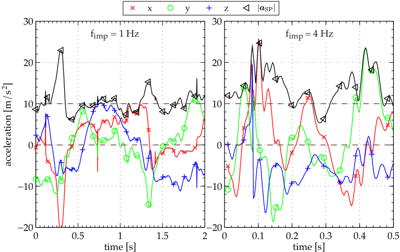
Figure 3: Sample acceleration time-series, $\bm{a}_{\text{SP}}(t)$, with the impellers counter-rotating at $f_{\text{imp}}=1\;\mathrm{Hz}$ (left) and $f_{\text{imp}}=4\;\mathrm{Hz}$ (right). Both samples last 2 integral times $T_{\text{int}}$.

Fig. 3 shows two sample time-series of the three components of the acceleration measured by the instrumented particle in the von Kármán flow, superimposed with the norm of the acceleration. Two different frequencies of the impellers are presented here: $1\,\mathrm{Hz}$ and $4\,\mathrm{Hz}$. The mean value of the norm fluctuates around $g=9.8\,\mathrm{m}\mathrm{/}\mathrm{s}\mathrm{{}^{2}}$, indicating that gravity is always measured by the accelerometer. Furthermore, the fluctuations of the norm increase with the impeller frequency. It is, however, difficult to compare the three components of the acceleration, either between each other or for different impeller frequencies. This is mainly due to the measurement of the gravity that is randomly projected on the three axes of the accelerometer as the particle rotates in the flow. It results in signals containing both contributions from the gravity and the particle’s translation, with no straightforward method to separate them. In other words, contrary to other methods (e.g. particle tracking velocimetry) it is not possible to obtain directly the characteristics of the particle motion. Hence, one needs to post-process the data to derive information about the statistics and the dynamics of the particle.

II.1 Analysis of the raw signal $a_{\text{SP}}$

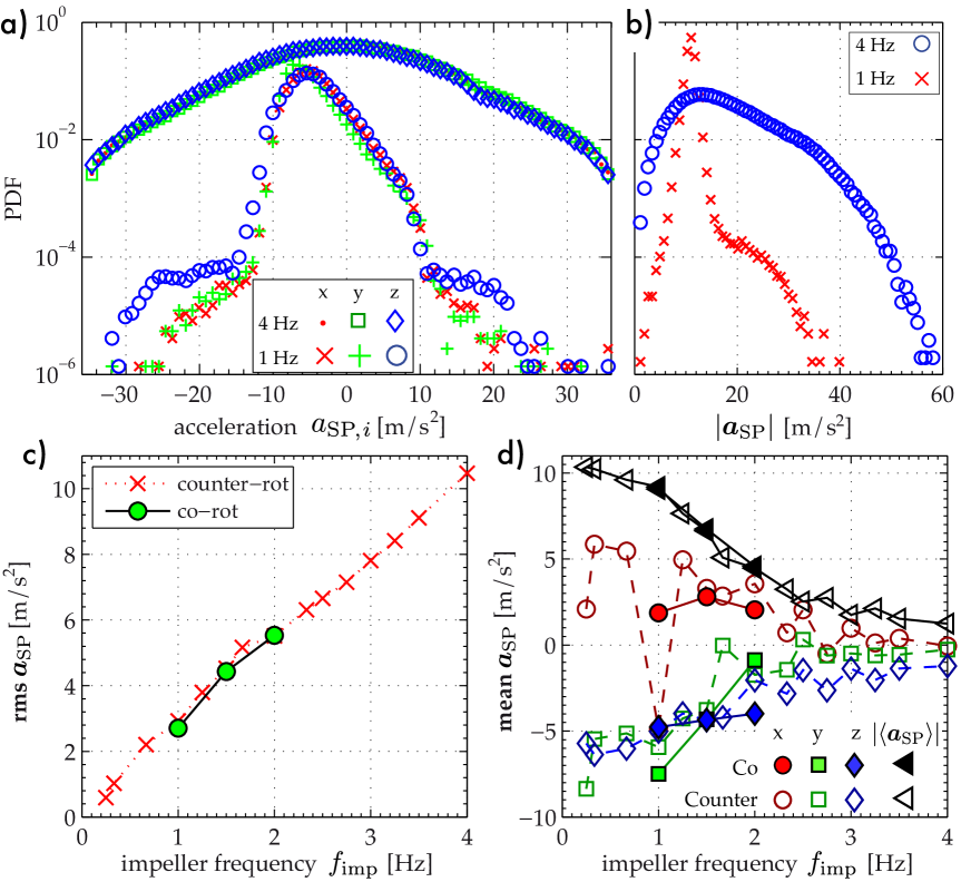
Figure 4: Top: Probability density functions of a) the components and b) the norm of the acceleration $\bm{a}_{\text{SP}}$ for two different impeller frequencies. For readability, the PDFs of acceleration components at $4\,\mathrm{Hz}$ have been arbitrarily shifted.  Bottom: Evolution of c) ${\small{\textbf{rms}}}\,{\bm{a}_{\text{SP}}}$ and d) $\left\langle\bm{a}_{\text{SP}}\right\rangle$ with the impeller frequency $f_{\text{imp}}$; filled symbols ($\circ$) indicate co-rotating impellers. In all cases the particle explored the flow for a sufficient amount of time for the statistics to converge. In good agreement with Eq. (2), $\left\lvert\left\langle\bm{a}_{\text{SP}}\right\rangle\right\rvert$ continuously decreases from $1g$ to $0g$ as the impeller frequency increases.

Fig. 4 shows different results of a basic statistical analysis of the acceleration signals, namely the PDFs of the three components and the norm of the acceleration for different impeller frequencies, and the fluctuating and mean values of the acceleration as a function of the impeller frequency. The accelerometer used in the smartPART saturates if one of the acceleration components exceeds $\pm 3.6g$, we exclude these points from the analysis. This removal diminishes the observed acceleration and the bias increases with the forcing. In the case of Fig. 4, almost $3\%$ of all data points were removed at $f_{\text{imp}}=4\;\mathrm{Hz}$, which is two orders of magnitude higher than for $f_{\text{imp}}=1\;\mathrm{Hz}$. Looking at the PDFs of the acceleration for a given impeller frequency (Fig. 4a), one can see that the three components give similar results for a wide range of acceleration values. However, the PDFs are very different from one frequency to another. Whereas at low impeller frequencies the PDFs are skewed and shifted, they become centered and symmetric with increasing impeller frequency. This evolution in shape can be explained by the particle’s mass distribution and imbalance. Although the particle is carefully prepared, its moment of inertia is not that of a solid sphere and the particle’s center of mass does not perfectly coincide with its geometrical center. Consequently, the particle becomes slightly out-of-balance, with a preferred orientation at low impeller frequency: the peaks then correspond to the projection of $\bm{g}$ on the axes in this preferred orientation and fluctuations around it. When the impeller frequency (and consequently the turbulence level) increases, the particle is able to explore all the possible orientations, meaning $\bm{g}$ is randomly projected in all directions, and the asymmetry disappears. The PDFs of the norm $\left\lvert\bm{a}_{\text{SP}}\right\rvert$ (Fig. 4b) also show this difference in shape, with a clear peak near the value $g$ (again, gravity is always measured by the 3D accelerometer), but with a narrow strong peak at low impeller speed and a more stretched PDF at high impeller speed.

The evolution of the fluctuations of acceleration (rms $\bm{a}_{\text{SP}}$) with the impeller frequency is given in Fig. 4c. Only one component of the acceleration is presented here for readability, since no preferred direction in any of the axes was found. This results in all three components rms values having the same behavior and amplitudes. One can see that surprisingly, the fluctuations of acceleration increase linearly with the frequency. That is in contrast to dimensional arguments that tell $\bm{a}_{\text{trans}}\propto f_{\text{imp}}^{2}$. Moreover, it is not possible to distinguish between the co- and counter-rotating regimes of the impellers.

Fig. 4d shows $\left\langle\bm{a}_{\text{SP}}\right\rangle$ as a function of the impeller frequency, $f_{\text{imp}}$, and the forcing. As expected the mean accelerations are becoming smaller with increasing impeller frequency. Indeed taking the average of Eq. (1) yields:

$$\begin{split}\left\langle\bm{a}_{\text{SP}}\right\rangle=\left\langle\smash{\underline{\underline{\mathbf{R}}}}\,\bm{g}\right\rangle+\left\langle\smash{\underline{\underline{\mathbf{R}}}}\,\bm{\bm{a}_{\text{trans}}}\right\rangle.\end{split}$$ (2)

If the particle explores continuously all the possible orientations, the mean vanishes; whereas a fixed orientation (i.e. no rotation) yields $\left\langle\bm{a}_{\text{SP}}\right\rangle=\smash{\underline{\underline{\mathbf{R}}}}\left(\bm{g}+\left\langle\bm{\bm{a}_{\text{trans}}}\right\rangle\right)$. This is what is observed in Fig. 4. In the case of weak turbulence (i.e. for smaller values of $f_{\text{imp}}$), the mean acceleration gives an estimate of gravity: $\left\langle\bm{a}_{\text{SP}}\right\rangle\approx\left\langle\smash{\underline{\underline{\mathbf{R}}}}\,\bm{g}\right\rangle$. However, for stronger turbulence and even if the mass distribution slightly induces a preferred direction, the particle can rotate freely around this axis, resulting in a vanishing mean acceleration when the impeller frequency increases: $\left\langle\bm{a}_{\text{SP}}\right\rangle\rightarrow 0$. In the latter case, contacts with impellers, walls, eddies, etc also help overpowering any preferred direction easily and force the particle to rotate. It can be noted that again, it is not possible to distinguish between the co- and counter-rotating regimes. Furthermore, the variance of a component $a_{\text{SP,i}}$ of $\bm{a}_{\text{SP}}$ depends strongly on its mean value, $\left\langle a_{\text{SP,i}}\right\rangle$. As explained before, gravity renders $\left\langle a_{\text{SP,i}}\right\rangle$ non-negligible. Additionally, we observe for weak turbulence levels ($f_{\text{imp}}\lesssim 1\;\mathrm{Hz}$) that particles are able to stay in an orientation for several seconds. Hence, a global mean of the complete time-series is not a meaningful quantity.

The direct study of the raw acceleration signal, $\bm{a}_{\text{SP}}$, only allows to conclude whether the particle rotates or not. It does not permit to disentangle the contributions of the gravity and the particle translation, and subsequently to have any precise insight on the flow. Other methods adapted to this problem are thus needed to extract informations from the instrumented particle related to its motion.

II.2 Moments of the acceleration due to the particle’s translation

In confined flows and provided the statistics are converged, it is $\left\langle\bm{a}_{\text{trans}}\right\rangle=0$. One is, therefore, interested in the PDF of $\bm{a}_{\text{trans}}$. Although, we mentioned we don’t have direct access to $\bm{a}_{\text{trans}}$ and its PDF, we can compute the even (central) moments of its PDF.

The variance of $\bm{a}_{\text{SP}}$ is

$$\begin{split}\left\langle\bm{a}_{\text{SP}}^{2}\right\rangle&=\left\langle\left\lvert\smash{\underline{\underline{\mathbf{R}}}}\,\bm{g}\right\rvert^{2}\right\rangle+\left\langle\left\lvert\smash{\underline{\underline{\mathbf{R}}}}\,\bm{a}_{\text{trans}}\right\rvert^{2}\right\rangle+2\left\langle\smash{\underline{\underline{\mathbf{R}}}}\,\bm{g}\cdot\smash{\underline{\underline{\mathbf{R}}}}\,\bm{a}_{\text{trans}}\right\rangle\\ &=g^{2}+\left\langle\bm{a}_{\text{trans}}^{2}\right\rangle+2\,g\left\langle a_{z}\right\rangle,\end{split}$$ (3)

where $a_{z}\equiv\bm{\hat{e}}_{z}\cdot\bm{\bm{a}_{\text{trans}}}$. It should be kept in mind, that each axis of the smartPART’s accelerometer is limited to $\pm 3.6\,g$, and possible events of higher acceleration are therefore not included in the analysis. The PDF of $\left\lvert\bm{a}_{\text{SP}}\right\rvert^{2}$ for different impeller frequencies is shown in Fig. 5a. As expected, a peak is clearly observed at $g^{2}$. One can also see that there are breaks in the slope at $\left\lvert\bm{a}_{\text{SP}}\right\rvert^{2}\approx(3.6\,g)^{2}$ and $\left\lvert\bm{a}_{\text{SP}}\right\rvert^{2}\approx 2\,(3.6\,g)^{2}$, corresponding to cases where one or two axes would saturate. Some information is inevitably lost, and to investigate the behavior at large $f_{\text{imp}}$, the sensor would have to be replaced with a different model supporting higher accelerations.

If the particle is neutrally buoyant and the flow is confined, one expects $\left\langle a_{z}\right\rangle=0$. We therefore obtain an estimate of the standard deviation (rms) of $\bm{a}_{\text{trans}}$:

$$\begin{split}a_{\text{rms}}\equiv\sqrt{\left\langle\bm{a}_{\text{trans}}^{2}\right\rangle}=\sqrt{\left\langle\bm{a}_{\text{SP}}^{2}\right\rangle-g^{2}}.\end{split}$$ (4)

$a_{\text{rms}}$ is independent of how gravity is projected on the axes of the accelerometer (in other words it is insensitive to the particle’s absolute orientation). Nevertheless, a bad calibration (e.g. caused by longterm drift or strong temperature change) can introduce a systematic offset to $a_{\text{rms}}$. Nevertheless, this bias can be minimized by calibrating the thermalized smartPART before the actual experiment. Fig. 5b depicts the evolution of $a_{\text{rms}}$ with the impeller frequency. In agreement with dimensional analysis, $a_{\text{rms}}\left(f_{\text{imp}}\right)$ describes a parabola, although one could also argue that $a_{\text{rms}}$ seems linear with ${f_{\text{imp}}}$ for $f_{\text{imp}}\geq 3\,\mathrm{Hz}$. As illustrated in Fig. 5a, this is caused by saturation of the accelerometer, which cuts off/underestimates high acceleration events present at these high turbulence level.

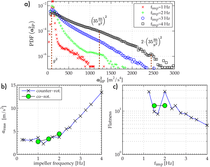
Figure 5: Moments of $\bm{a}_{\text{trans}}$. a) $\operatorname{PDF}\left(\bm{a}_{\text{SP}}^{2}\right)$ at different impeller frequencies. The 3 vertical lines mark gravity and the saturation of one or two accelerometer axes. b) and c) : RMS and fourth moment of $\bm{a}_{\text{trans}}$ as a function of the impeller frequency. $a_{\text{rms}}(f_{\text{imp}})=\sqrt{\left\langle\left\lvert\bm{a}_{\text{SP}}(f_{\text{imp}})\right\rvert^{2}\right\rangle-g^{2}}$.

Similarly to the variance, one can estimate the fourth central moment of $\bm{a}_{\text{trans}}$. It is

$$\begin{split}\big{\langle}\left\lvert\bm{a}_{\text{SP}}\right\rvert^{4}\big{\rangle}\;&=\;\left\langle\left[g^{2}+\bm{a}_{\text{trans}}^{2}+2\,g\,a_{z}\right]\left[g^{2}+\bm{a}_{\text{trans}}^{2}+2\,g\,a_{z}\right]\right\rangle\\ \quad&=g^{4}+\big{\langle}\left\lvert\bm{a}_{\text{trans}}\right\rvert^{4}\big{\rangle}+2\,g^{2}\,\left\langle\bm{a}_{\text{trans}}^{2}\right\rangle+4\,g^{2}\left\langle a_{z}^{2}\right\rangle+4\,g^{3}\left\langle a_{z}\right\rangle+4\,g\left\langle\left\lvert\bm{a}_{\text{trans}}\right\rvert^{2}a_{z}\right\rangle.\end{split}$$ (5)

Assuming no preferred direction in $\bm{\bm{a}_{\text{trans}}}$, as found for small particles in a windtunnel Voth et al. (2002) and verified for solid particles of size comparable to the integral length scale in the same apparatus Zimmermann (2012), one has $4g^{2}\left\langle a_{z}^{2}\right\rangle\approx 4/3\,g^{2}\,\bm{a}_{\text{trans}}^{2}$. Again, the terms $\left\langle a_{z}\right\rangle$, $4\,g^{3}\left\langle a_{z}\right\rangle$ and $4g\big{\langle}\left\lvert\bm{\bm{a}_{\text{trans}}}\right\rvert^{2}a_{z}\big{\rangle}$ are expected to vanish in the case of confined flows. Eq. (5) then simplifies to

$$\big{\langle}\left\lvert\bm{a}_{\text{SP}}\right\rvert^{4}\big{\rangle}\approx g^{4}+\big{\langle}\left\lvert\bm{a}_{\text{trans}}\right\rvert^{4}\big{\rangle}+\frac{10}{3}g^{2}a_{\text{rms}}^{2}.$$ (6)

The flatness, $F(\bm{a}_{\text{trans}})$, is defined as:

$$\begin{split}F\left(\bm{a}_{\text{trans}}\right)=\frac{\big{\langle}\left\lvert\bm{a}_{\text{trans}}\right\rvert^{4}\big{\rangle}}{\left\langle\bm{a}_{\text{trans}}^{2}\right\rangle^{2}}=\frac{\big{\langle}\left\lvert\bm{a}_{\text{SP}}\right\rvert^{4}\big{\rangle}-g^{4}-\frac{10}{3}g^{2}a_{\text{rms}}^{2}}{a_{\text{rms}}^{4}}.\end{split}$$ (7)

As shown in Fig. 5c we observe a flatness of the order of $10$ in our von Kármán flow, which is close to the flatness obtained in the case of much smaller particles Qureshi et al. (2007) and to our finding for solid particles of similar size Zimmermann (2012). The uncertainty in the flatness can partially be attributed to an uncertainty in $g$ and stems from the resolution, noise and measurement range of the smartPART, but also from the particle’s weak drift. It is furthermore biased by contacts with impellers and walls. More surprisingly, the flatness decreases with the forcing. This decline is again due to the limited measurement range of the accelerometer used: at high accelerations the sensor saturates and thereby sets $\operatorname{PDF}\big{(}\bm{a}_{\text{trans}}\,\big{|}\,\left\lvert a_{\text{SP,}i}\right\rvert>3.6g\big{)}=0$. Since the flatness is the fourth moment of the PDF and as such highly sensitive to strong accelerations, we find a decrease whereas solid large spheres in the same flow have an increasing flatness Zimmermann (2012). We also conclude that calculating moments of higher order is out of reach.

It is remarkable, that based only on the second and fourth moment of $\bm{a}_{\text{trans}}$  one cannot clearly distinguish between a counter-rotating and a co-rotating flow although these two forcings induce two clearly different large scale flow structures. Similar behavior has been found for solid spheres of comparable size in the same flow Zimmermann (2012), too. It should be noted that the energy injection rates for the two ways of driving the flow differ by only a factor of 2: the co-rotating forcing is highly turbulent, too. In addition, in vicinity of the disks the flow has a strong contribution of the centrifugal pumping of the blades on the impellers and the flow configurations are comparable in that region.

II.3 Auto-correlation functions

In order to distinguish between the two regimes, we now turn to the auto-correlation of the acceleration time-series to estimate correlation time scales of the flow. Ideally, one would want to compute the auto-correlation of the translational force, e.g. $\left\langle\bm{a}_{\text{trans}}\left(t\right)\cdot\bm{a}_{\text{trans}}\left(t+\tau\right)\right\rangle$, but again the constantly changing orientation of the smartPART blocks any direct access to $\bm{a}_{\text{trans}}\left(t\right)$ and quantities derived thereof. We therefore need to find quantities, which are either not altered by the orientation of the smartPART or extract information on its rotation.

II.3.1 An Auto-correlation invariant to the rotation of the sensor

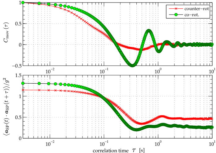
Figure 6: Top: Rotation-invariant auto-correlation function $C_{\text{mov}}\left(\tau\right)$ (Eq. (8) after rescaling); the auto-correlation significantly differs between counter- and co-rotating impellers. Bottom: Rotation-sensitive auto-correlation function $\left\langle\bm{a}_{\text{SP}}(t)\cdot\bm{a}_{\text{SP}}(t+\tau)\right\rangle/g^{2}$. In all cases the impeller frequency is $1.5\;\mathrm{Hz}$. A logarithmic scale is chosen for the abscissae to display both short and long time contributions to the correlations.

In the spirit of Eq. (3) and Eq. (5) one can construct the auto-correlation function of the magnitude of $\bm{a}_{\text{SP}}$. It is:

$$\begin{split}&\left\langle\left\lvert\bm{a}_{\text{SP}}(t)\right\rvert^{2}\left\lvert\bm{a}_{\text{SP}}(t+\tau)\right\rvert^{2}\right\rangle\\ &\quad=\;\left\langle\left[g^{2}+\bm{a}_{\text{trans}}^{2}(t)+2\,\bm{g}\cdot\bm{a}_{\text{trans}}(t)\right]\left[g^{2}+\bm{a}_{\text{trans}}^{2}(t+\tau)+2\,\bm{g}\cdot\bm{a}_{\text{trans}}(t+\tau)\right]\right\rangle\\ &\quad=\left\langle\left\lvert\bm{a}_{\text{trans}}(t)\right\rvert^{2}\left\lvert\bm{a}_{\text{trans}}(t+\tau)\right\rvert^{2}\right\rangle+g^{4}+2g^{2}\,\left\langle\bm{a}_{\text{trans}}^{2}\right\rangle+4g^{2}\left\langle{a_{z}(t)}\,{a_{z}(t+\tau)}\right\rangle\\ &\qquad+4\,g^{3}\left\langle a_{z}\right\rangle+2g\left\langle\left\lvert\bm{a}_{\text{trans}}(t+\tau)\right\rvert^{2}a_{z}(t)\right\rangle+2g\left\langle\left\lvert\bm{a}_{\text{trans}}(t)\right\rvert^{2}a_{z}(t+\tau)\right\rangle\\ &\quad\approx\left\langle\left\lvert\bm{a}_{\text{trans}}(t)\right\rvert^{2}\left\lvert\bm{a}_{\text{trans}}(t+\tau)\right\rvert^{2}\right\rangle+g^{4}+2\,g^{2}a_{\text{rms}}^{2}+4g^{2}\left\langle{a_{z}(t)}\;{a_{z}(t+\tau)}\right\rangle.\end{split}$$ (8)

Again, the terms containing $a_{z}\equiv\bm{\hat{e}}_{z}\cdot\bm{\bm{a}_{\text{trans}}}$ are expected to have zero mean. However, the last term on the right-hand side of Eq. (8) does not vanish for $\tau\approx 0$, becoming $4g^{2}\left\langle{a_{z}(t)}\;{a_{z}(t+\tau)}\right\rangle=4g^{2}\left\langle\left\lvert a_{z}\right\rvert^{2}\right\rangle$. Assuming no preferred direction in $\bm{a}_{\text{trans}}$ this can be approximated as $4/3\,g^{2}\,a_{\text{rms}}^{2}$. In contrast to Eq. (8), we preferably compute the autocorrelation of the fluctuations around the mean $\left\langle\bm{a}^{2}_{SP}\right\rangle$. Hence, the autocorrelation of the norm can be negative. We further normalize the auto-correlation such that it is $1$ at $\tau=0$. After rescaling, we refer to this rotation-invariant quantity as $C_{\text{mov}}\left(\tau\right)$.

Fig. 6 displays $C_{\text{mov}}\left(\tau\right)$ for the co- and counter-rotating regime at an impeller frequency of $1.5\;\mathrm{Hz}$. The auto-correlation of the counter-rotating forcing is well approximated by a sum of exponential decays. In contrast thereto, we observe that co-rotating impellers correspond to an auto-correlation function showing a damped oscillation, i.e.   the smartPART observes the longer coherence in the large scale motion of the flow. This is in agreement with Eulerian measurements, where pressure probes were mounted in a von Kármán flow: whereas the counter-rotating flow produces typical pressure spectra, the same probe in the co-rotating case yields a spectrum which peaks at multiples of the impeller frequency. Similar behavior has been reported for the magnetic field in a von Kármán flow Volk et al. (2006) filled with liquid Gallium (in that particular case the co-rotating regime was created by rotating only one impeller).

Summing up, $\big{\langle}\left\lvert\bm{a}_{\text{SP}}(t)\right\rvert^{2}\left\lvert\bm{a}_{\text{SP}}(t+\tau)\right\rvert^{2}\big{\rangle}$ is insensitive to the particular tumbling/rotational dynamics of the particle and it gives necessary information to determine the type of flow. We also checked that this result is not altered by a possible imbalance of the particle.

II.3.2 An Auto-correlation related to the tumbling of the particle

One can further focus on the rotation of the particle by considering the product:

$$\begin{split}&\left\langle\bm{a}_{\text{SP}}(t)\cdot\bm{a}_{\text{SP}}(t+\tau)\right\rangle\\ &\quad=\left\langle\left[\smash{\underline{\underline{\mathbf{R}}}}\left(t\right)\,\left(\bm{g}+\bm{\bm{a}_{\text{trans}}}(t)\right)\right]\cdot\left[\smash{\underline{\underline{\mathbf{R}}}}\left(t+\tau\right)\,\left(\bm{g}+\bm{\bm{a}_{\text{trans}}}(t+\tau)\right)\right]\right\rangle\\ &\quad=\left\langle\left[\smash{\underline{\underline{\mathbf{R}}}}^{T}\big{(}t+\tau\big{)}\cdot\smash{\underline{\underline{\mathbf{R}}}}\big{(}t\big{)}\,\left(\bm{g}+\bm{\bm{a}_{\text{trans}}}(t)\right)\right]\cdot\left[\left(\bm{g}+\bm{\bm{a}_{\text{trans}}}(t+\tau)\right)\right]\right\rangle\\ &\quad=\left\langle\bm{g}\cdot\left[\smash{\underline{\underline{\mathbf{T}}}}(t,\tau)\bm{g}\right]\right\rangle+\left\langle\left[\smash{\underline{\underline{\mathbf{T}}}}(t,\tau)\bm{\bm{a}_{\text{trans}}}(t)\right]\cdot\bm{\bm{a}_{\text{trans}}}(t+\tau)\right\rangle+\left\langle\left[\smash{\underline{\underline{\mathbf{T}}}}(t,\tau)\bm{g}\right]\cdot\bm{\bm{a}_{\text{trans}}}(t+\tau)\right\rangle+\left\langle\left[\smash{\underline{\underline{\mathbf{T}}}}(t,\tau)\bm{\bm{a}_{\text{trans}}}(t)\right]\bm{g}\right\rangle\\ &\quad\approx g^{2}\left\langle\hat{\bm{e}}_{z}\cdot\left[\smash{\underline{\underline{\mathbf{T}}}}(t,\tau)\hat{\bm{e}}_{z}\right]\right\rangle+\left\langle\left[\smash{\underline{\underline{\mathbf{T}}}}(t,\tau)\cdot\bm{\bm{a}_{\text{trans}}}(t)\right]\bm{\bm{a}_{\text{trans}}}(t+\tau)\right\rangle,\end{split}$$ (9)

where the term $\smash{\underline{\underline{\mathbf{T}}}}(t,\tau)\equiv\smash{\underline{\underline{\mathbf{R}}}}^{T}\big{(}t+\tau\big{)}\smash{\underline{\underline{\mathbf{R}}}}\big{(}t\big{)}$ is a rotation matrix related to the instantaneous angular velocity $\bm{\omega}$ of the particle as explained in Ref. Zimmermann et al. (2011a). Again, the two terms containing products of $\bm{g}$ and $\bm{a}$ vanish if the particle is neutrally buoyant. The term $g^{2}\left\langle\hat{\bm{e}}_{z}\cdot\left[\smash{\underline{\underline{\mathbf{T}}}}(t,\tau)\hat{\bm{e}}_{z}\right]\right\rangle$ is related to the tumbling of a spherical particle Wilkinson and Pumir (2011). In contrast to the other auto-correlation Eq. (8), one cannot subtract a mean value prior to computing $\left\langle\bm{a}_{\text{SP}}(t)\cdot\bm{a}_{\text{SP}}(t+\tau)\right\rangle$. To estimate the ratio between $g^{2}\left\langle\hat{e}_{z}\cdot\left[\smash{\underline{\underline{\mathbf{T}}}}(t,\tau)\hat{e}_{z}\right]\right\rangle$ and $\left\langle\left[\smash{\underline{\underline{\mathbf{T}}}}(t,\tau)\bm{\bm{a}_{\text{trans}}}(t)\right]\cdot\bm{\bm{a}_{\text{trans}}}(t+\tau)\right\rangle$ it is helpful to normalize by $g^{2}$.

If $\left\langle\left[\smash{\underline{\underline{\mathbf{T}}}}(t,\tau)\cdot\bm{\bm{a}_{\text{trans}}}(t)\right]\bm{\bm{a}_{\text{trans}}}(t+\tau)\right\rangle$ becomes uncorrelated, $\left\langle\bm{a}_{\text{SP}}(t)\cdot\bm{a}_{\text{SP}}(t+\tau)\right\rangle$ does not necessarily vanish. If uncorrelated ($\tau\gg T_{\text{int}}$):

$$\begin{split}\left\langle\bm{a}_{\text{SP}}(t)\cdot\bm{a}_{\text{SP}}(t+\tau)\right\rangle&\cong g^{2}\left\langle\smash{\underline{\underline{\mathbf{R}}}}\left(t\right)\hat{\bm{e}}_{z}\cdot\smash{\underline{\underline{\mathbf{R}}}}\left(t+\tau\right)\hat{\bm{e}}_{z}\right\rangle\\ &=g^{2}\left\langle\smash{\underline{\underline{\mathbf{R}}}}\hat{\bm{e}}_{z}\right\rangle^{2}\geqslant 0\end{split}$$ (10)

That means $\left\langle\bm{a}_{\text{SP}}(t)\cdot\bm{a}_{\text{SP}}(t+\tau)\right\rangle$ approaches a plateau whose height is determined by the average orientation of the particle. In analogy to $C_{\text{mov}}$, one can then subtract $g^{2}\left\langle\smash{\underline{\underline{\mathbf{R}}}}\hat{\bm{e}}_{z}\right\rangle^{2}$ and rescale $\left\langle\bm{a}_{\text{SP}}(t)\cdot\bm{a}_{\text{SP}}(t+\tau)\right\rangle$, which is termed $C_{\text{tumb}}\left(\tau\right)$ in the following.

The lower plot in Fig. 6 depicts $\left\langle\bm{a}_{\text{SP}}(t)\cdot\bm{a}_{\text{SP}}(t+\tau)\right\rangle/g^{2}$ for the two forcing regimes at an impeller frequency of $1.5\;\mathrm{Hz}$. In agreement with Eq. (10), a plateau is reached for both forcings.

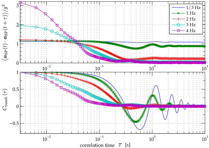
Figure 7: Top: Dependence of $\left\langle\bm{a}_{\text{SP}}(t)\cdot\bm{a}_{\text{SP}}(t+\tau)\right\rangle/g^{2}$ on the impeller frequency for counter-rotating impellers;  Bottom: Same data after subtracting the plateau and rescaling.

To investigate the role of the plateau we plot the auto-correlation of the particle for increasing $f_{\text{imp}}$ in Fig. 7. For $f_{\text{imp}}\lesssim 1\;\mathrm{Hz}$ one finds little change with the plateau at almost $1$. For $f_{\text{imp}}\approx 2\;\mathrm{Hz}$ the plateau drops but is still non-zero. The value of the plateau diminishes with further increase in $f_{\text{imp}}$. At the same frequency range we observe that the PDFs of the components of $\bm{a}_{\text{SP}}$ become centered and symmetric (cf. Fig. 4). $C_{\text{tumb}}\left(\tau\right)$ – i.e. Eq. (9) after subtracting the plateau and rescaling – accesses the fluctuations around a mean value and is shown in the bottom plot of Fig. 7. We find that $C_{\text{tumb}}\left(\tau\right)$ evolves from a long-time correlated oscillatory shape at low impeller speeds to an exponential decay at high $f_{\text{imp}}$.

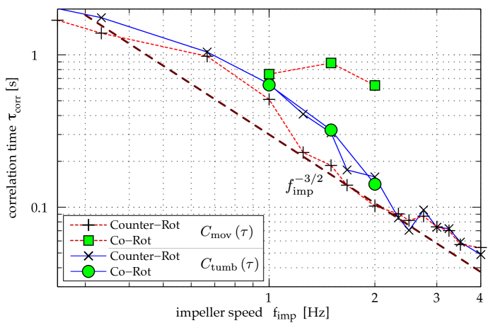
Figure 8: Characteristic flow time scale $\tau_{\text{corr}}$ determined from rotation-invariant, $C_{\text{mov}}\left(\tau\right)$, and rotation-sensitive, $C_{\text{tumb}}\left(\tau\right)$, auto-correlation function. Whereas both autocorrelation functions yield comparable $\tau_{\text{corr}}$  for counter-rotating driving, we find that their results are well distinct in the case of co-rotating impellers. The dashed line indicates a $f_{\text{imp}}^{-3/2}$ power-law, as suggested by the scaling of the Kolmogorov time scale ($\tau_{\eta}\propto\varepsilon^{-1/2}$ and $\varepsilon\propto f_{\text{imp}}^{3}$).

II.3.3 Time scales

The autocorrelation functions contain time-scales which are related to the movement of the particle in the flow. We identify two scenarios for the autocorrelations ($C_{\text{mov}}\left(\tau\right)$ and $C_{\text{tumb}}\left(\tau\right)$): as illustrated in Fig. 6, they are either conducting a weakly- or a critically-damped oscillation. With increasing turbulence level the oscillation is gradually changing towards the critically damped case and for high propeller speeds ($f_{\text{imp}}>2.5\,\mathrm{Hz}$) no damped oscillation is observed (cf. Fig. 7). In order to extract meaningful time-scales we, therefore, fit two test-functions to each autocorrelation function. The functions are the transient solution of a weakly damped harmonic oscillator:

$$\begin{split}f_{w}(\tau)=a_{0}\,\exp\left(-\tau/\tau_{\text{corr}}\right)\cdot\sin\left(2\pi f_{\text{osc}}+\phi_{0}\right),\end{split}$$ (11)

and of a critically damped one:

$$f_{d}(\tau)=\exp\left(-\tau/\tau_{\text{corr}}\right)\cdot\left(a_{0}+a_{1}\,\tau\right).$$ (12)

$\tau_{\text{corr}},f_{\text{osc}}$ and $a_{0},a_{1},\phi_{0}$ are fit-parameters. We return $\tau_{\text{corr}}$ and (if available) $f_{\text{osc}}$ from the test-function which performs better in approximating the autocorrelation. $C_{\text{mov}}\left(\tau\right)$ and $C_{\text{tumb}}\left(\tau\right)$ access motion and tumbling of the particle, respectively, and yield thus different time scales. For the oscillatory case, $f_{\text{osc}}$ contributes additional details on the particle’s motion.

Fig. 8 shows $\tau_{\text{corr}}$ as a function of the impeller frequency and driving. We find that both rotation-invariant (Eq. (8)) and rotating-sensitive (Eq. (9)) function find very similar correlation times in the counter-rotating configuration. Moreover, $\tau_{\text{corr}}$ of the particle follows roughly a $f_{\text{imp}}^{-3/2}$ power-law as suggested by the scaling of the Kolmogorov time scale (it is $\tau_{\eta}\propto\varepsilon^{-1/2}$ and $\varepsilon\propto f_{\text{imp}}^{3}$). Furthermore, $\tau_{\text{corr}}$ obtained from the rotation-sensitive function is independent of the way we drive the flow. In contrast thereto, the rotation-invariant function gives correlation times, $\tau_{\text{corr}}$, which are larger and only little dependent on the impeller frequency if the impellers are co-rotating. That means one can distinguish co- from counter-rotating forcing by comparing the timescales of the two auto-correlation functions.

Concerning the oscillation frequency $f_{\text{osc}}$ (not shown in figure), we find that the rotation-sensitive autocorrelation senses the tumbling/wobbling of the particle, which is directly related to the particle’s imbalance and independent of the flow. The rotation-invariant autocorrelation on the other hand shows an oscillation frequency following the impeller frequency with $f_{\text{osc}}\sim\frac{2}{3}f_{\text{imp}}$.

III Discussion

After briefly presenting the working principle of an instrumented particle measuring Lagrangian accelerations, we established a mathematical framework based on statistical moments and auto-correlation functions to analyze turbulent flows from the particle’s signals. In particular, we developed methods which are either invariant or sensitive to the rotation of the particle and its sensor in the flow. These methods perform well within the wide range of tested turbulence levels. With a smartPART one gets access to correlation time scales of the flow, as well as the variance and flatness of the (translational) acceleration. Comparing the rotation-sensitive and the rotation-invariant autocorrelation allows distinguishing between different flow regimes, notably detecting long-time correlated large vortex structures as shown here with the co-rotating forcing of a von Kármán flow. In contrast to particle tracking methods the instrument particle returns one long trajectory instead of many short realizations. To that extent, it has to be noted that we limited our analysis to the extraction of global flow features. In order to follow the evolution of a slowly changing flow in time, these methods can, however, be extended to sliding windows. Work on adaptive filtering techniques is ongoing, in particular we are testing the Empirical Mode Decomposition, which might be able to separate the different contributions of the signal and thereby get even deeper insight into the flow.

We emphasize that after usage the particle can be easily extracted from the flow and then be reused and that by virtue of the developed mathematical framework no optical access is needed. The instrumented particle can therefore shed some light into flows that are not or hardly accessible up to now. Due to its continuous transmission one flow configuration can be characterized within $\sim 30\,\mathrm{min}$. This technique is an interesting tool for a fast quantification of a wide range of flows as they are found both in research labs and industry.