Dynamical Singularities of Glassy Systems in a Quantum Quench

Abstract

We present a prototype of behavior of glassy systems driven by quantum dynamics in a quenching protocol by analyzing the random energy model in a transverse field. We calculate several types of dynamical quantum amplitude and find a freezing transition at some critical time. The behavior is understood by the partition-function zeros in the complex temperature plane. We discuss the properties of the freezing phase as a dynamical chaotic phase, which are contrasted to those of the spin-glass phase in the static system.

I INTRODUCTION

Phase transitions are one of the most fascinating topics in statistical physics. After the long investigations, equilibrium phase transitions are clarified as singularities of free energies and become known to be treatable in the current framework of statistical mechanics Onsager:44 ; Yang:52 ; Fisher:64 . To analyze those singularities, sophisticated techniques and concepts, such as the renormalization group theory and the scaling hypothesis, have been founded and nowadays equilibrium phase transitions of classical systems are fairly well understood. On the other hand, phase transitions or dynamical singularities of quantum systems are far less understood, though rising interests in quantum computation require better comprehension of those phenomena. Recent experimental developments enable to observe time evolutions of quantum many-body systems in detail Greiner:02 ; Kinoshita:06 ; Sadler:06 , which also demands better theoretical clarifications of dynamical behavior of quantum systems.

Recently, dynamical singularities of quantum systems in a typical experimental set up, the so-called quantum quench, are focused Pollmann:10 ; Kolodrubetz:11 ; Heyl:12 . In the set up, a quantum system, whose Hamiltonian with a parameter $\Gamma$ is written as $\mathcal{H}(\Gamma)$, is prepared in a quantum state $|\psi_{0}\rangle$ dominated by $\mathcal{H}(\Gamma_{0})$, and the parameter is suddenly changed as $\Gamma_{0}\to\Gamma_{1}$ at $t=0$. After the quench, the wave function of the system at time $t\geq 0$ is given by

$$|\psi(t)\rangle=e^{-it\mathcal{H}(\Gamma_{1})}|\psi_{0}\rangle.$$ (1)

Due to the sudden quench, the behavior of this wave function can be drastically different from the one in adiabatic process. It is actually reported that another energy scale different from the adiabatic one exists and dominates the system, which can lead to novel non-analyticity in dynamical behavior Pollmann:10 ; Kolodrubetz:11 ; Heyl:12 . Interestingly, those dynamical singularities can be analyzed by the theory of zeros of equilibrium partition function Yang:52 ; Fisher:64 ; Heyl:12 . This provides a possibility to analyze a wide range of dynamical singularities of quantum systems, with the current maturity of the theory of zeros.

Based on this possibility, in this paper, we provide a prototype of dynamical singularities of glassy systems. For this, we focus on the so-called random energy model (REM) Derrida:80 ; Gross:84 in a transverse field (TREM) introducing quantum nature Goldschmidt:90 ; Obuchi:07 ; Jorg:08 ; Takahashi:11 . Despite its simplicity, the REM is known to show many nontrivial properties of glassy systems and is treated as an ideal platform to study systems with many metastable states Kirkpatrick:89 ; Bryngelson:87 , which naturally motivates us to firstly investigate the TREM to examine dynamical singularities of glassy systems. In addition, the distribution of the partition-function zeros is well known in the REM Derrida:91 ; Takahashi:11 , and we can expect that the present analysis reveals a clear relation between the dynamical singularities and zeros.

II MODEL

The Hamiltonian of the TREM is defined as the limit of the fully-connected Ising spin-glasses (SGs) with $p$-body interactions $\mathcal{H}=H_{p}+H_{g}$ where

$$H_{p}=-\sum_{i_{1}<\cdots<i_{p}}J_{i_{1}\cdots i_{p}}\sigma_{i_{1}}^{z}\cdots\sigma_{i_{p}}^{z},$$ (2)

$$H_{g}=-\Gamma\sum_{i=1}^{N}\sigma_{i}^{x}.$$ (3)

$\sigma^{x,z}$ are Pauli matrices, $N$ is the number of spins, and the interaction $J_{i_{1}\cdots i_{p}}$ is independent identically distributed (i.i.d.) from Gaussian with zero mean and variance $p!/2N^{p-1}$. The REM is produced by taking the limit $\lim_{p\to\infty}H_{p}=H_{\rm REM}$ Derrida:80 . Energy levels of $H_{\rm REM}$ lose the correlations among each other in the limit $p\to\infty$, and thus energy levels of the REM Hamiltonian $H_{\rm REM}$ become i.i.d. Gaussian variables with zero mean and variance $N/2$. The TREM Hamiltonian is given by $\mathcal{H}_{\rm TREM}=H_{\rm REM}+H_{g}$, and hence in the $\sigma^{z}$ representation the diagonal elements are random Gaussian variables coming from $H_{\rm REM}$, and the off-diagonal ones arise from $H_{g}$.

The TREM has three thermodynamic phases Goldschmidt:90 . One is the classical paramagnetic (CP) phase which dominates the system for small $\Gamma$ and large temperature $T=1/\beta$, and another one is the SG phase appearing at low $T$ and small $\Gamma$. The last one is the quantum paramagnetic (QP) phase emerging for large $\Gamma$. The free energy densities are given by

$$f=\left\{\begin{array}[]{lc}-\frac{\beta}{4}-\frac{\ln 2}{\beta}&\mbox{for CP}\\ -\sqrt{\ln 2}&\mbox{for SG}\\ -\frac{1}{\beta}\ln(2\cosh\beta\Gamma)&\mbox{for QP}\end{array}\right..$$ (7)

First-order phase transitions from QP to CP or SG phases occur at critical values $\Gamma_{\rm c}(T)$. Clearly, the CP and SG phases do not depend on $\Gamma$, and also the QP phase is not influenced by $H_{\rm REM}$ since $f$ is completely identical to $-(1/N\beta)\ln{\rm Tr}\,\exp(-\beta H_{g})$. These imply the strong simplicity of the TREM. Actually, Jörg et al. showed that perturbations from $\Gamma=0$ and $\Gamma=\infty$ do not change the eigenfunctions in both two cases in the thermodynamic limit Jorg:08 , which can be schematically written as

$${\rm Tr}\,e^{-\beta\mathcal{H}_{\rm TREM}}\to\left\{\begin{array}[]{ll}{\rm Tr}\,e^{-\beta H_{\rm REM}}&\mbox{for}\ \Gamma<\Gamma_{\rm c}(T)\\ {\rm Tr}\,e^{-\beta H_{g}}&\mbox{for}\ \Gamma\geq\Gamma_{\rm c}(T)\end{array}\right..$$ (10)

This property makes the following analysis extremely simple.

III OVERLAPS

III.1 Return amplitude

Hereafter, we consider a quantum quench protocol from large to small $\Gamma$, and examine the dynamical singularities in the TREM. Following Ref. Heyl:12 , we investigate the return amplitude $G(t)\equiv\langle\psi_{0}|\psi(t)\rangle=\langle\psi_{0}|\exp(-it\mathcal{H})|\psi_{0}\rangle$, especially focusing on the ground state for large $\Gamma$. Namely, we put $|\psi_{0}\rangle=|{\rm QP}\rangle$ where $|{\rm QP}\rangle$ denotes the ground state of $H_{g}$ which includes all the $\sigma^{z}$-basis with an equal weight $1/\sqrt{2^{N}}$.

Thanks to the specialty of the TREM (10), we can easily say $|G(t)|^{2}=1$ if the quench does not go across the critical value $\Gamma_{\rm c}(0)$. On the other hand, when the quench goes across $\Gamma_{\rm c}$, $|G(t)|^{2}$ is expected to exponentially decrease as time $t$ grows, i.e. $|G(t)|^{2}\propto\exp(-Ng(t))$. To assess the rate function $g(t)$, Eq. (10) again makes the problem quite simple. Using this, we can rewrite

$$G(t)=\langle{\rm QP}|e^{-itH_{\rm REM}}|{\rm QP}\rangle=\frac{1}{2^{N}}Z_{\rm REM}(it),$$ (11)

where we write the partition function of the REM under the inverse temperature $\beta$ as $Z_{\rm REM}(\beta)$. Hence, $g(t)$ is directly related to the free energy of the REM under the imaginary temperature.

The calculation of Eq. (11) is a simple task in the REM. Using the spectral representation $G(t)=2^{-N}\sum_{n=1}^{2^{N}}\exp(-iE_{n}t)$, we divide the square of the amplitude $|G(t)|^{2}$ into time-dependent and -independent parts. Taking the random average, we obtain

$$[|G(t)|^{2}]\sim\exp(-N\ln 2)+\exp(-Nt^{2}/2).$$ (12)

We naively expect that the first term is much smaller than the second one since the former involves $2^{N}$-terms and the latter $2^{N}(2^{N}-1)\sim 2^{2N}$. However, when $t$ becomes large enough, the second Gaussian term is considerably smaller than the first term and the time-independent part becomes important. Thus, we have a dynamical phase transition. The rate function is given by

$$g(t)=\left\{\begin{array}[]{ll}\frac{t^{2}}{2}&\mbox{for}\ t\leq t_{\rm c}=\sqrt{2\ln 2}\\ \ln 2&\mbox{for}\ t>t_{\rm c}\end{array}\right..$$ (15)

We see that the amplitude freezes at $t=t_{\rm c}$.

III.2 Generalized overlap

To obtain further information about $|\psi(t)\rangle$, overlaps with other wave functions are also useful. As such reference wave functions, we here introduce wave functions $|\beta\rangle$ reflecting finite temperature properties

$$|\beta\rangle=\frac{e^{-\beta H_{\rm REM}/2}|{\rm QP}\rangle}{\sqrt{\langle{\rm QP}|e^{-\beta H_{\rm REM}}|{\rm QP}\rangle}},$$ (16)

and consider the overlap with $|\psi(t)\rangle$

$$G_{1/2}(\beta,t)\equiv\langle\beta|\psi(t)\rangle=\frac{1}{\sqrt{2^{N}}}\frac{Z_{\rm REM}\left(\frac{\beta}{2}+it\right)}{\sqrt{Z_{\rm REM}(\beta)}}.$$ (17)

We can easily confirm that the quantum-mechanical average of physical quantities commutative with $H_{\rm REM}$ by $|\beta\rangle$ completely agrees with the statistical-mechanical average at inverse temperature $\beta$ Somma:07 ; Morita:08 . On the other hand, concerning any non-commutative quantity $A$, the quantum-mechanical average by $|\beta\rangle$ involves non-diagonal contributions, i.e. $\sum_{n\neq m}e^{-\beta(E_{n}+E_{m})/2}\langle{E_{n}}|A|E_{m}\rangle$, which leads to a deviation from the correct statistical-mechanical average. However, it is known that the correct average, vanishing of non-diagonal contributions, can be reproduced by appropriately extending the Hilbert space of $|\beta\rangle$, the extension of which is called thermofield dynamics Fano:52 ; Suzuki:98 ; Tasaki:98 . We can use this extension, but it does not change the following discussion and hence we just use $|\beta\rangle$ hereafter. As another way to reproduce the correct statistical-mechanical average, it is known that the introduction of random numbers is also useful Goldstein:06 ; Sugiura:12 . This prescription is interesting but involves some technical difficulties, and again we do not use the prescription.

To treat $G(t)$ and $G_{1/2}(\beta,t)$ in the same manner, we introduce a generalized overlap with index $k$ as

$$G_{k}(\beta,t)=\frac{1}{(2^{N})^{1-k}}\frac{Z_{\rm REM}\left(k\beta+it\right)}{(Z_{\rm REM}(\beta))^{k}}.$$ (18)

This reduces to Eq. (17) at $k=1/2$, and $G_{k}(0,t)=G_{0}(\beta,t)=G(t)$. Furthermore, $G_{1}(\beta,t)$ denotes the thermal average of the time evolution operator $\exp(-itH_{\rm REM})$ and is worth studying.

IV Analysis and Result

To handle the average $[|G_{k}|^{2}]$, we use the replica method

$$[|G_{k}|^{2}] = \frac{1}{(2^{N})^{2(1-k)}}\lim_{n_{1}\to 1}\lim_{n_{2}\to-2k}\Bigl{[}Z_{\rm REM}^{n_{1}}(k\beta+it)$$ (19)

$$\times Z_{\rm REM}^{n_{1}}(k\beta-it)Z_{\rm REM}^{n_{2}}(\beta)\Bigr{]}.$$

We treat $n_{1}$ and $n_{2}$ as integers and consider the analytic continuation to real variables after the calculation. For readers familiar with the replica method, the introduction of $n_{1}$ may seem to be strange since the limiting value is unity, at which the replica symmetry breaking (RSB) effect does not appear vanHemmen:79 . However, we stress that the introduction of $n_{1}$ is needed to construct the RSB solution in the numerator of Eq. (18), which is necessary for the correct solution.

The calculation goes along the standard manner Takahashi:11 and the result is expressed in terms of the order parameter matrix $Q$ with the size $n_{1}+n_{1}+n_{2}$. We obtain $[|G_{k}|^{2}]=\lim_{n_{1}\to 1}\lim_{n_{2}\to-2k}\exp(-N\tilde{g})$ where

$$\tilde{g} = -\frac{k^{2}\beta^{2}-t^{2}}{4}\sum_{a,b}^{n_{1}}\left(q_{ab}^{(+)}+q_{ab}^{(-)}\right)-\frac{\beta^{2}}{4}\sum_{a,b}^{n_{2}}q_{ab}^{(2)}$$ (20)

$$-\frac{ik\beta t}{2}\sum_{a,b}^{n_{1}}\left(q_{ab}^{(+)}-q_{ab}^{(-)}\right)-\frac{k^{2}\beta^{2}+t^{2}}{2}\sum_{a,b}^{n_{1}}q_{ab}^{(+-)}$$

$$-\frac{\beta(k\beta+it)}{2}\sum_{a}^{n_{1}}\sum_{b}^{n_{2}}q_{ab}^{(+2)}-\frac{\beta(k\beta-it)}{2}\sum_{a}^{n_{1}}\sum_{b}^{n_{2}}q_{ab}^{(-2)}$$

$$+2(1-k)\ln 2-s.$$

$q=0$ or 1 represents a matrix element of $Q$ and is determined by the extremized condition. The superscript denotes the block in the matrix $Q$: $+$ ($-$) is for the first (second) block with the size $n_{1}$, and 2 is for the third with $n_{2}$. The subscript denotes replica numbers in each block. The number of configurations for a given order parameter $Q$ is denoted by $\exp(Ns)$ and $s$ plays the role of the entropy density.

Following the discussions in Takahashi:11 , we can find four possible saddle-point solutions. In the replica symmetric (RS) level, we have two solutions and the rate function $g_{k}=\lim_{n_{1}\to 1}\lim_{n_{2}\to-2k}\tilde{g}$ is calculated as follows:

P1

This solution is denoted by the identity matrix $Q=1$. That is: $q_{ab}^{(+)}=q_{ab}^{(-)}=q_{ab}^{(2)}=\delta_{a,b}$ and zero for the other elements. The corresponding entropy is $s=(2n_{1}+n_{2})\ln 2$. Then, the rate function is

$$g_{k}=\frac{1}{2}t^{2}+\frac{k(1-k)}{2}\beta^{2}.$$ (21)

P2

The first and second blocks have an identical configuration as $q_{ab}^{(+)}=q_{ab}^{(-)}=q_{ab}^{(2)}=q_{ab}^{(+-)}=\delta_{a,b}$ Takahashi:11 . The entropy is given by $s=(n_{1}+n_{2})\ln 2$ and we obtain

$$g_{k}=k\left(\frac{1}{2}-k\right)\beta^{2}+\ln 2.$$ (22)

Other two solutions are obtained by assuming the one-step replica symmetry breaking (1RSB). In the present problem, we divide $n_{1}$ replicas into $n_{1}/m_{1}$ blocks of size $m_{1}$, and $q_{ab}$ takes $1$ if $a$ and $b$ are in the same block and $0$ otherwise. The $n_{2}$ replicas are similarly divided into $n_{2}/m_{2}$ blocks of size $m_{2}$. Two different solutions emerges according to the value of $q^{(+-)}$:

1RSB1

$q^{(+-)}=0$. The entropy is $s=(2n_{1}/m_{1}+n_{2}/m_{2})\ln 2$ and the rate function becomes

$$g_{k}(m_{1},m_{2}) = 2(1-k)\ln 2-\frac{k^{2}\beta^{2}-t^{2}}{2}m_{1}-\frac{2\ln 2}{m_{1}}$$ (23)

$$+\frac{k\beta^{2}}{2}m_{2}+\frac{2k\ln 2}{m_{2}}.$$

Extremization with respect to $m_{2}$ give $m^{*}_{2}=2\sqrt{\ln 2}/\beta\equiv\beta_{\rm c}/\beta$. On the other hand, the extremization of $m_{1}$ gives a physically-unacceptable condition $m_{1}=\beta_{\rm c}/\sqrt{k^{2}\beta^{2}-t^{2}}$. Hence, we get one possible solution in this ansatz

$$g_{k}(1,m^{*}_{2})=\frac{1}{2}t^{2}-\frac{1}{2}(k\beta-\beta_{\rm c})^{2}+2(1-k)\ln 2.$$ (24)

1RSB2

We assume that $q^{(+-)}$ takes the same form as $q^{(+)}$ and $q^{(-)}$. Then,

$$g_{k}(m_{1},m_{2}) = 2(1-k)\ln 2-k^{2}\beta^{2}m_{1}-\frac{\ln 2}{m_{1}}$$ (25)

$$+\frac{k\beta^{2}}{2}m_{2}+\frac{2k\ln 2}{m_{2}}.$$

The extremization gives $m^{*}_{1}=\beta_{\rm c}/2k\beta$ and $m^{*}_{2}=\beta_{\rm c}/\beta$, both of which are acceptable in contrast to the 1RSB1 case. Hence, we have three possible solutions in this case

$$g_{k}(1,m^{*}_{2})=-\left(k\beta-\frac{\beta_{\rm c}}{2}\right)^{2}+2(1-k)\ln 2,$$ (26)

$$g_{k}(m^{*}_{1},1)=\frac{k}{2}(\beta-\beta_{\rm c})^{2}+2(1-k)\ln 2,$$ (27)

$$g_{k}(m^{*}_{1},m^{*}_{2})=2(1-k)\ln 2.$$ (28)

Comparing the above solutions and considering the RSB constraint $0\leq m_{1},m_{2}\leq 1$, we specify the dominating solutions, to find that the set of solutions depend on $k$. For $1\leq k$, the solutions are P1, P2, and 1RSB2 with $(m_{1},m_{2})=(m^{*}_{1},1)$, $(m^{*}_{1},m^{*}_{2})$. For $1/2\leq k<1$, 1RSB1 is included to the above four solutions. For $k<1/2$, 1RSB2 with $(1,m^{*}_{2})$ appears instead of that with $(m^{*}_{1},1)$. We show the phase diagram at $k=1$ and $1/2$ in Fig. 1.

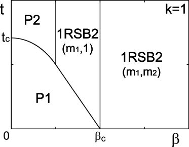
Figure 1: Phase diagram for $k=1$ and $k=1/2$ on $\beta$-$t$ plane.

In P1 and 1RSB1 phases, the rate function depends on $t$ and the amplitude decays in $t$. Then, in P2 and 1RSB2 phases, the amplitude ceases to decrease and is frozen to a fixed value.

V Discussions

Figure 2: The rate function $g(t)$ in the discrete REM with $N=80$ and $\alpha=1.3$. Each line represents the result from a single sample.

Figure 3: $g_{1/2}(\beta,t)$ in the same calculation as Fig. 2.

Our result of $[|G_{k}|^{2}]$ is compared with the distribution of the partition-function zeros in the complex-$\beta$ plane. The zeros of $Z_{\rm REM}(\beta)$ with complex $\beta$ was calculated in Refs. Derrida:91 ; Takahashi:11 and a similar phase diagram including the P1, P2, and 1RSB phases was found. In the present problem, the rate function $g_{k}$ for a given $\beta$ is frozen to a fixed value in the P2 and 1RSB2 phases and it seems to be hard to recognize the difference between these two phases. However, it is known that the density of zeros two-dimensionally distributes in the P2 phase but no zeros exist in the 1RSB2 phase Takahashi:11 ; Derrida:91 , which implies a qualitative difference.

Concerning the 1RSB2 phase, it is easy to interpret the plateau of $g_{k}$ with respect to $t$, since this corresponds to the SG phase which is well understood. The SG transition of the REM occurs as the freezing of the system into the ground state. This directly leads to $g_{k}$ in the 1RSB2 phase since the ground state of the REM, $|\rm SG\rangle$, gives the overlap $|\langle{\rm SG}|\psi(t)\rangle|^{2}=1/2^{N}$.

On the other hand, such a freezing does not occur in the P2 phase. Instead, it is expected that the dominant states for the free energy rapidly switch as $t$ changes, which implies a kind of chaos emerges in the overlap in the P2 phase. This speculation is based on the recently-proposed relation between the distribution of zeros and the chaos effect of SGs Obuchi:12 . The chaos effect of SGs means that the spin configuration drastically changes as the physical parameters, such as temperature or external field, slightly vary Bray:87 . In the mean-field level, the chaos effect of SGs can be interpreted as the changes of dominant thermodynamic pure states Rizzo:06 , which produces the two-dimensionally distributing zeros Obuchi:12 . These considerations naturally lead to the connection between a kind of chaos in dynamic behavior and the P2 phase.

To confirm this assertion, we numerically calculate the rate function. From a technical reason, we treat the discrete version of the REM, where $2^{N}$-energy levels are denoted by $M+1$-discrete binomially-distributed variables Mourkarzel:91 ; Ogure:04 . This model gives a phase transition for $\alpha=M/N>1$, whose physical nature is the same as the REM. We plot the rate function $g(t)$, which is equivalent to $g_{1/2}(\beta=0,t)$, at $\alpha=1.3$ in Fig. 2. The plotted curves are taken from 10 samples of random distributions. We can find that for small $t$, where the P1 phase dominates, all the samples give an identical smooth curve, while for large $t$ singular fluctuations depending on samples appear around the plateau of the P2 phase $g(t)=\ln 2$. This singular behavior is just the chaotic state mentioned above. To make further comparison, in Fig. 3 we also plot the data at $\beta=8$ where the 1RSB2 phase dominates. Although the sample dependence is large both for the P2 and the 1RSB2 cases, there is no singular fluctuations for the latter case. This difference originates from the partition-function zeros, which are present and absent in the P2 and 1RSB2 phases, respectively.

Note that the dynamical singularities investigated above are not specific to the REM. Actually, the presence of the P2 phase is confirmed in other SG models Obuchi:12 ; Matsuda:10 . It is relatively easy to demonstrate this fact for the case $k=1/2$ and $\beta=0$, and we here show the result of the Sherrington-Kirkpatrick (SK) model Sherrington:75 , which is the standard mean-field model of SGs and corresponds to the $p=2$ case in Eq. (2). The explicit formula of $g(t)=g_{1/2}(\beta=0,t)$ becomes

$$g(t)=\frac{t^{2}}{2}+\frac{t^{2}}{2}q^{2}-\ln\cosh\left(qt^{2}\right),$$ (29)

where the order parameter $q$ is determined through

$$q=\tanh\left(qt^{2}\right).$$ (30)

We note that there is no need to use the replica method in the case of $\beta=0$ since the denominator in Eq. (18) reduces to a constant. The order parameter $q$ represents the overlap between two spaces and corresponds to $q^{(+-)}$ in the analysis of the previous section. We plot $g(t)$ in Fig. 4, to find the transition of second-order at $t_{\rm c}=1$.

Figure 4: The analysis of $[|G_{1/2}(\beta=0,t)|^{2}]$ in the SK model. The solid line represents the rate function $g(t)$. The singularity appears at $t=1$ which can be understood from the behavior of the order parameter $q$ (dashed line) and the cusp of $dg(t)/dt$ (dotted line).

The rate function $g(t)$ is more smooth than that of the REM and still increases $t>t_{\rm c}$, implying the SK model do not freeze into a small number of states even at $t>t_{\rm c}$, which is in contrast to the REM. This fact might mean that the chaotic effect more drastically affect the dynamical behavior in the SK model, which should be confirmed in future works.

Finally, we discuss the possibility of observing the dynamical singularities in experiments. Let us consider only the case $k=1/2$ and $\beta=0$. What we have calculated so far is the probability that the time-evolved wave function becomes the state $|\psi_{0}\rangle$ with the maximum magnetization in the $x$ direction. Thus, generally speaking, we can experimentally estimate this probability by observing $x$-direction magnetization of $|\psi(t)\rangle$ many times and counting the number of times where the $x$-direction magnetization is maximized, and hence we can see the singularity in the probability in principle. This is a kind of quantum tomography. Admittedly, this is quite difficult since the probability tends to be very small, which requires an enormous number of preparations and observations of the wave function. Thus, another pathway to observe this probability, if exists, is desired. Although exploration of the pathway is beyond our purpose in the present paper, we here address some interesting possibility. In equilibrium statistical mechanics, the celebrated Einstein’s fluctuation theory tells us that the probability, or the rate function, of occurrence of atypical fluctuations can be directly connected to the free energy which is more easily observed in experiments. This connection recently inspires an exploration of similar relation in non-equilibrium phenomena, and some positive results are obtained Nemoto:11 ; Nemoto:12 . Similar results might be obtained for purely quantum systems, which can contribute to the above problem in quantum tomography.

VI Conclusion

In this paper, we have studied the dynamical singularities of glassy systems in a quantum quench protocol, by treating the REM as an illustrative example. To widely investigate this problem, we have proposed a class of wave functions reflecting finite-temperature properties, and have defined and studied overlaps between the finite-temperature wave function and the time-evolved one in a quantum quench, not only the overlap with the initial state. To analyze the overlaps in a general way, we have invented a formulation based on the replica method and applied it to the REM. The rate functions of the overlaps show freezing behavior at critical time $t_{\rm c}$ which vanishes for low temperatures due to the emergence of the SG phase. We have also discussed the connection between the freezing behavior and the zeros of the partition function, to find a chaotic behavior for $t>t_{\rm c}$ detected by the zeros. The presence of this chaotic behavior is common for a wide range of SG models, and a demonstration on the SK case has been also presented.

Possibility of observing the dynamical singularities in experiments has been also discussed. Although it is in general possible to observe the singularities in experiments, some difficulty should present due to the small probability of the desired event. To resolve this problem, a better theoretical comprehension among non-equilibrium statistical physics and quantum many-body dynamics will be needed. There is still a gap between statistical physics and quantum physics communities, and we hope that this paper contributes to filling this gap and encouraging the investigation of this interdisciplinary research field.

References

- (1) L. Onsager, Phys. Rev. 65, 117 (1944).
- (2) C. N. Yang and T. D. Lee, Phys. Rev. 87, 404 (1952); T. D. Lee and C. N. Yang, Phys. Rev. 87, 410 (1952).
- (3) M. E. Fisher, in Lectures in Theoretical Physics, edited by W. E. Brittin (University of Colorado Press, Boulder, 1965), Vol. 7c.
- (4) M. Greiner, O. Mandel, T. Esslinger, T. Hänsch, and I. Bloch, Nature 419, 51 (2002).
- (5) T. Kinoshita, T. Wenger, and D. Weiss, Nature 440, 900 (2006).
- (6) L. E. Sadler, J. M. Higbie, S. R. Leislie, M. Vengalattore, and D. M. Stamper-Kurn, Nature 443, 312 (2006).
- (7) F. Pollmann, S. Mukerjee, A. G. Green, and J. E. Moore, Phys. Rev. E 81, 020101 (2010).
- (8) M. Kolodrubetz, B. K. Clark, and D. A. Huse, Phys. Rev. Lett. 109, 015701 (2012).
- (9) M. Heyl, A. Polkovnikov, and S. Kehrein, arXiv:1206.2505.
- (10) B. Derrida, Phys. Rev. Lett. 45, 79 (1980).
- (11) D. J. Gross and M. Mézard, Nucl. Phys. B 240, 431 (1984).
- (12) Y. Y. Goldschmidt, Phys. Rev. B 41, 4858 (1990).
- (13) T. Obuchi, H. Nishimori, and D. Sherrington, J. Phys. Soc. Jpn. 76, 054002 (2007).
- (14) T. Jörg, F. Krzakala, J. Kurchan, and A. C. Maggs, Phys. Rev. Lett. 101, 147204 (2008).
- (15) K. Takahashi, J. Phys. A: Math. Theor. 44, 235001 (2011).
- (16) T. R. Kirkpatrick, D. Thirumalai, and P. G. Wolynes, Phys. Rev. A 40, 1045 (1989).
- (17) J. D. Bryngelson and P. G. Wolynes, Proc. Natl. Acad. Sci. USA 84, 7524 (1987).
- (18) B. Derrida, Physica A 177, 31 (1991).
- (19) R. D. Somma, C. D. Batista, and G. Ortiz, Phys. Rev. Lett. 99, 030603 (2007).
- (20) S. Morita and H. Nishimori, J. Math. Phys. 49, 125210 (2008).
- (21) U. Fano, Rev. Mod. Phys. 29, 74 (1952).
- (22) M. Suzuki, J. Stat. Phys. 42, 1047 (1998).
- (23) H. Tasaki, Phys. Rev. Lett. 80, 1373 (1998).
- (24) S. Goldstein, J. L. Lebowitz, R. Tumulka, and N. Zanghì, Phys. Rev. Lett. 96, 050403 (2006).
- (25) S. Sugiura and A. Shimizu, Phys. Rev. Lett. 108, 240401 (2012).
- (26) J. L. van Hemmen and R. G. Palmer, J. Phys. A: Math. Gen. 12, 563 (1979).
- (27) T. Obuchi and K. Takahashi, J. Phys. A: Math. Theor. 45, 125003 (2012).
- (28) A. J. Bray and M. A. Moore, Phys. Rev. Lett. 58, 57 (1987).
- (29) T. Rizzo and H. Yoshino, Phys. Rev. B 73, 064416 (2006).
- (30) C. Moukarzel and N. Parga, Physica A 177, 24 (1991).
- (31) K. Ogure and Y. Kabashima, Prog. Theor. Phys. 111, 661 (2004).
- (32) Y. Matsuda, M. Müller, H. Nishimori, T. Obuchi, and A. Scardicchio, J. Phys. A: Math. Theor. 43, 285002 (2010).
- (33) D. Sherrington and S. Kirkpatrick, Phys. Rev. Lett. 35, 1792 (1975).
- (34) T. Nemoto and S.-I. Sasa, Phys. Rev. E 83, 030105 (2011); ibid. 84, 061113 (2011).
- (35) T. Nemoto, Phys. Rev. E 85, 061124 (2012).