Quantum discord amplification induced by quantum phase transition via a cavity-Bose-Einstein-condensate system

Abstract

We propose a theoretical scheme to realize a sensitive amplification of quantum discord (QD) between two atomic qubits via a cavity-Bose-Einstein condensate (BEC) system which was used to firstly realize the Dicke quantum phase transition (QPT) [Nature 464, 1301 (2010)]. It is shown that the influence of the cavity-BEC system upon the two qubits is equivalent to a phase decoherence environment. It is found that QPT in the cavity-BEC system is the physical mechanism of the sensitive QD amplification.

Quantum discord (QD)  Ollivier2001 ; Henderson2003 is considered to be a more general resource than quantum entanglement in quantum information processing Datta2008 ; Lanyon2008 ; Roa2011 ; Li2012 ; Datta2009 ; Madhok2012 . A nonzero QD in some separable states is responsible for the quantum computational efficiency of deterministic quantum computation with one pure qubit Datta2008 ; Lanyon2008 ; Knill1998 and also has been considered as an useful resource in quantum locking  Datta2009 and quantum state discrimination Roa2011 ; Li2012 . On the other hand, any realistic quantum systems interact inevitably with their surrounding environments, which introduce quantum noise into the systems. As an useful resource, it is interesting that QD can be amplified by the quantum noise. We find the QD does be amplified for two non-interacting qubits immersed in a common phase decoherence environment Yuan2010 . Especially, when the two qubits are identical, the phase decoherence can induce a stable amplification of the initially-prepared QD for certain $X$-type states. In this paper, we propose a scheme to realize the controllable QD amplification of two atomic qubits by making use of an artificial phase decoherence environment consisting of a cavity-Bose-Einstein condensate (BEC) system.

The Dicke model Dicke1954 ; EmaryC2003 describes a larger number of two-level atoms interacting with a single cavity field mode. As increasing atom-filed coupling, the model predicts a QPT Sachdev1999 from the normal phase, which the atoms are in the ground state associated with vacuum field state, to the super-radiant phase, which both the atoms and field have collective excitations. Recently, a cavity-Bose-Einstein condensate (BEC) system is employed to firstly realize the Dicke quantum phase transition (QPT) experimentally and to explore symmetry breaking at the Dicke QPT  Baumann2010 . Meanwhile, the QPT system usually displays ultra-sensitivity in its dynamical evolution near the quantum critical point Hepp1973 ; Wang1973 ; Emary2003 ; Quan2006 ; Huang2009 , which has been confirmed by a NMR experiment Zhang2008 . The purpose of this paper is to show that the QD of two initially correlated atomic qubits can be sensitively amplified via the cavity-BEC system near the critical point. We show that the cavity-BEC system can form an artificial phase decoherence environment for the two atomic qubits, and the QD of the two atomic qubits can be amplified by adjusting the QPT parameter of the cavity-BEC system.

The physical system under our consideration is shown in Fig. 1. A BEC with $N$ identical two-level ${}^{87}Rb$ atoms is confined in a ultrahigh-finesse optical cavity. The atoms interact with a single cavity model of frequency $\omega_{c}$ and a transverse pump field of frequency $\omega_{p}$. We consider a situation that the frequency $\omega_{c}$ and $\omega_{p}$ are detuned far from the atomic resonance frequency $\omega_{A}$ so that the dutunings far exceed the rate of atomic spontaneous emission, the atoms only scatter photons either along or transverse to the cavity axis. Before the pump field turns on, atoms in the BEC are supposed to be in the zero-momentum state $|p_{x},p_{z}\rangle=|0,0\rangle$. As soon as one turns on the pump field, via the photon scattering of the pump and cavity fields, some atoms are excited into the momentum sates $|p_{x},p_{z}\rangle=|\pm k,\pm k\rangle=\sum_{\upsilon_{1},\upsilon_{2}=\pm 1}|\upsilon_{1}k,\upsilon_{2}k\rangle$ (hereafter, we take $\hbar=1$.) due to the conservation of momentum, where $k$ is the wave-vector, which is approximated to be equal on the cavity and pump fields. The two momentum states with $|0,0\rangle$ and $|\pm k,\pm k\rangle$ are regarded as two levels of the ${}^{87}Rb$ atom with energy separation $\omega_{0}=k^{2}/m$, where $m$ is the mass of ${}^{87}Rb$ atom. Defined the collective operators $\hat{J_{z}}=\sum_{i}|\pm k,\pm k\rangle\langle\pm k,\pm k|$, $\hat{J_{+}}=\hat{J_{-}^{{\dagger}}}=\sum_{i}|\pm k,\pm k\rangle\langle 0,0|$ with the index $i$ labelling the atoms, the cavity- BEC is described by the Dick model  Baumann2010 ; Baumann2011

$$\hat{H}_{1}=\omega\hat{a}^{{\dagger}}\hat{a}+\omega_{0}\hat{J}_{z}+\frac{\lambda}{\sqrt{N}}\left(\hat{a}+\hat{a}^{{\dagger}}\right)(\hat{J_{+}}+\hat{J_{-}}),$$ (1)

where $\hat{a}^{{\dagger}}(\hat{a})$ is the creation (annihilation) operator of the cavity field. $\omega=-\Delta_{c}+U_{0}N/2$ is effective frequency of the cavity field including the frequency shift induced by the BEC under the frequency of pump field rotating frame, where $\Delta_{c}=\omega_{p}-\omega_{c}$ is the dutuning between pump field and cavity field and $U_{0}=g_{0}^{2}/\Delta$ is the frequency shift of a single atom with maximally cavity field coupling strength $g_{0}$ and detuning $\Delta=\omega_{p}-\omega_{A}$. $\lambda=\sqrt{N}g_{0}\Omega_{p}/2\Delta$ is the coupling strength induced by the cavity field and pump field with $\Omega_{p}$ denoting the maximum pump Rabi frequency which can be adjusted by the pump power.

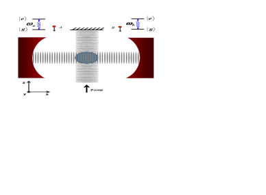
Figure 1: (Color online) Schematic of our physical system: Two atomic qubits $A$ and $B$ with energy separation $\omega_{A}$ and $\omega_{B}$ are, respectively, injected into the cavity in which a atomic BEC couples to a single cavity field and a transverse pump field.

We consider such a situation that the two atomic qubits pass through the cavity at the same time and interact with the single cavity field, the expression of the Hamiltonian reads as

$$\hat{H}_{2}=\omega\hat{a}^{{\dagger}}\hat{a}+\frac{\omega_{A}}{2}\hat{\sigma}_{z}^{A}+\frac{\omega_{B}}{2}\hat{\sigma}_{z}^{B}+\left(g_{A}\hat{a}^{{\dagger}}\hat{\sigma}_{-}^{A}+g_{B}\hat{a}^{{\dagger}}\hat{\sigma}_{-}^{B}+H.c\right),$$ (2)

where $\hat{\sigma}^{A(B)}_{z}=\left|e\right\rangle\left\langle e\right|-\left|g\right\rangle\left\langle g\right|$ is pauli operator with $\left|e\right\rangle$ and $\left|g\right\rangle$ being the excited and ground states. $\sigma^{A(B)}_{+}(\sigma^{A(B)}_{-})$ is the raising operator(lowering operator). $g_{A(B)}$ is the coupling strength between the atomic qubit A(B) and the cavity field, $\omega_{A(B)}$ is the energy separation. Here we have made a rotating wave approximation. If the atomic qubit is far-off-resonant with the cavity field satisfying the detuning $\Delta_{A(B)}=\omega_{A(B)}-\omega$ is much large than the corresponding coupling coupling strength $g_{A(B)}$, one can use the Fr$\ddot{\mathrm{o}}$hlich-Nakajima transformation Fr1950 ; Naka1955 to make the Hamiltonian in Eq. (2) become the following expression

$$\hat{H}_{2}^{{}^{\prime}}=\frac{1}{2}\omega_{A}^{{}^{\prime}}\hat{\sigma}_{z}^{A}+\frac{1}{2}\omega_{B}^{{}^{\prime}}\hat{\sigma}_{z}^{B}+\left(\omega+\delta_{A}\hat{\sigma}_{z}^{A}+\delta_{B}\hat{\sigma}_{z}^{B}\right)\hat{a}^{{\dagger}}\hat{a},$$ (3)

where $\omega_{A(B)}^{{}^{\prime}}=\omega_{A(B)}+\delta_{A(B)}$ with $\delta_{A(B)}=g^{2}_{A(B)}/\Delta_{A(B)}$ being the frequency shift induced by the scattering between cavity field and atomic qubit A(B). Then the effective Hamiltonian describing the two atomic qubits passing through the cavity-BEC system is

$$\hat{H}_{eff}=\frac{1}{2}\omega_{A}^{{}^{\prime}}\hat{\sigma}_{z}^{A}+\frac{1}{2}\omega_{B}^{{}^{\prime}}\hat{\sigma}_{z}^{B}+\left(\delta_{A}\hat{\sigma}_{z}^{A}+\delta_{B}\hat{\sigma}_{z}^{B}\right)\hat{a}^{{\dagger}}\hat{a}+\hat{H}_{1}.$$ (4)

Now we consider the dynamics of the two atomic qubits passing through the cavity-BEC system. We assume the two atomic qubits are initially prepared in a class of state with maximally mixed marginals ($\hat{\rho}^{A(B)}=\hat{I}^{A(B)}/2$) described by the three-parameter $X$-type density matrix $\hat{\rho}_{s}(0)=1/4(\hat{I}^{AB}+\sum_{i=1}^{3}c_{i}\hat{\sigma}_{i}^{A}\otimes\hat{\sigma}_{i}^{B})$, where $\hat{I}^{AB}$ is the identity operator in the Hilbert space of the two atomic qubits, $i=1,2,3$ mean $x,y,z$ correspondingly, and $c_{i}$ ($0\leq\left|c_{i}\right|\leq 1$) are real numbers satisfying the unit trace and positivity conditions of the density operator $\hat{\rho}_{s}(0)$. The cavity-BEC system is initially in the ground state $|G\rangle$ of the Hamiltonian in Eq. (1). The dynamic evolution of the total system is controlled by the Hamiltonian in Eq. (4). The density operator of the total system at time $t$ is written as $\rho_{T}(t)=U(\hat{\rho}_{s}(0)\otimes|G\rangle\langle G|)U^{{\dagger}}$ with $U=e^{-i\hat{H}_{eff}t}$. After tracing the degree of freedom of the cavity-BEC system, we obtain the reduced density of the two atomic qubits

$$\hat{\rho}_{s}(t)=\frac{1}{4}\left(\begin{array}[]{cccc}1+c_{3}&0&0&\mu(t)D_{1}(t)\\ 0&1-c_{3}&\nu(t)D_{2}(t)&0\\ 0&\nu^{*}(t)D^{*}_{2}(t)&1-c_{3}&0\\ \mu^{*}(t)D^{*}_{1}(t)&0&0&1+c_{3}\end{array}\right),$$ (5)

where we have introduced the following parameters

$$\mu(t) = (c_{1}-c_{2})e^{-i(\omega^{{}^{\prime}}_{A}+\omega^{{}^{\prime}}_{B})t},\hskip 5.69046pt\nu(t)=(c_{1}+c_{2})e^{-i(\omega^{{}^{\prime}}_{A}-\omega^{{}^{\prime}}_{B})t},$$

$$D_{1}(t) = \langle G|e^{i\hat{H}_{ee}t}e^{-i\hat{H}_{gg}t}|G\rangle,\hskip 5.69046ptD_{2}(t)=\langle G|e^{i\hat{H}_{eg}t}e^{-i\hat{H}_{ge}t}|G\rangle,$$ (6)

with

$$\hat{H}_{ee} = \delta_{1}\hat{a}^{{\dagger}}\hat{a}+\hat{H}_{1},\hat{H}_{gg}=-\delta_{1}\hat{a}^{{\dagger}}\hat{a}+\hat{H}_{1},\delta_{1}=\delta_{A}+\delta_{B}$$

$$\hat{H}_{eg} = \delta_{2}\hat{a}^{{\dagger}}\hat{a}+\hat{H}_{1},\hat{H}_{ge}=-\delta_{2}\hat{a}^{{\dagger}}\hat{a}+\hat{H}_{1},\delta_{2}=\delta_{A}-\delta_{B}.$$ (7)

We consider the situation that two atomic qubits pass through the cavity field region in a very short time of satisfying the conditions $\delta_{1}t\ll 1$ and $\delta_{2}t\ll 1$. In fact, according to Ref. Baumann2010 , the waist of the cavity field is 25 $\mu m$, the effective frequency shift $\delta_{A}$, $\delta_{B}$ are about 100 Hz, above conditions are well satisfied if injected velocity of the atomic qubits meets $v\gg 10^{-3}$ m/s. By the short time approximation, the factors $|D_{1}(t)|$, $|D_{2}(t)|$ can be derived as

$$|D_{1}\left(t\right)|=\exp\left(-2\gamma\delta_{1}^{2}t^{2}\right),|D_{2}\left(t\right)|=\exp\left(-2\gamma\delta_{2}^{2}t^{2}\right),$$ (8)

where the decay factor $\gamma=\left\langle\left(\hat{a}^{{\dagger}}\hat{a}\right)^{2}\right\rangle-\left\langle\hat{a}^{{\dagger}}\hat{a}\right\rangle^{2}$ is the cavity photon number fluctuation (PNF) in the ground state $|G\rangle$ Huang2009 .

From Eq. (5) we can see that the cavity-BEC system only affects off-diagonal elements of the density for the two atomic qubits, hence it is equivalently a phase decoherence environment for the two atomic qubits. That is, the cavity-BEC system constitutes an artificial phase decoherence environment of the two qubits. The QPT parameter of the cavity-BEC system $\lambda$ is a controllable parameter of the artificial environment. It’s worth noting that when the effective frequency shift $\delta_{A}$, $\delta_{B}$ are equal, i.e, $\delta_{2}=0$, a decoherence free space in the basis $\{|ge\rangle,|eg\rangle\}$ appears.

In order to obtain the detailed form of the PNF $\gamma$, in the following we give the ground state $|G\rangle$ according to the Ref. EmaryC2003 . Utilizing the Holstein-Primakoff transformation Holstein1940 $\hat{J}_{+}=\hat{c}^{{\dagger}}\sqrt{2j-\hat{c}^{{\dagger}}\hat{c}},\hat{J}_{-}=\sqrt{2j-\hat{c}^{{\dagger}}\hat{c}}\hat{c},\hat{J}_{z}=\hat{c}^{{\dagger}}\hat{c}-j$, where$j=N/2$ , the Hamiltonian of the Eq. (1) is further reduce to

$$\hat{H}_{1}=\omega\hat{a}^{{\dagger}}\hat{a}+\omega_{0}\hat{c}^{{\dagger}}\hat{c}+\lambda\left(\hat{a}+\hat{a}^{{\dagger}}\right)\left(\hat{c}^{{\dagger}}\sqrt{1-\frac{\hat{c}^{{\dagger}}\hat{c}}{2j}}+H.c.\right).$$ (9)

When the coupling strength $\lambda$ is smaller than the critical coupling strength $\lambda_{c}=\sqrt{\omega\omega_{0}}/2$, i.e., $\lambda<\lambda_{c}$, the system is in the normal phase where the BEC and the cavity field have low excitations. While when the coupling strength is larger than the critical strength, i.e., $\lambda>\lambda_{c}$, the system is in the super-radiant phase where both the BEC and the cavity field have collective excitations in the order of the atom number $N$.

In the normal phase at the thermodynamic limit $j\rightarrow\infty$, neglecting terms with $j$ in the denominator, Hamiltonian (9) becomes

$$\hat{H}_{1}=\omega\hat{a}^{{\dagger}}\hat{a}+\omega_{0}\hat{c}^{{\dagger}}\hat{c}+\lambda\left(\hat{a}+\hat{a}^{{\dagger}}\right)\left(\hat{c}+\hat{c}^{{\dagger}}\right),$$ (10)

where we omit the constant term. The Hamiltonian in Eq. (10) can be diagonalized as

$$\hat{H}_{1}=\varepsilon_{-}\hat{d}_{1}^{{\dagger}}\hat{d}_{1}+\varepsilon_{+}\hat{d}_{2}^{{\dagger}}\hat{d}_{2}$$ (11)

by the Bogoliubov transformation

$$\hat{a}^{{\dagger}} = f_{1}\hat{d}_{1}^{{\dagger}}+f_{2}\hat{d}_{1}+f_{3}\hat{d}_{2}^{{\dagger}}+f_{4}\hat{d}_{2},$$ (12)

$$\hat{c}^{{\dagger}} = h_{1}\hat{d}_{1}^{{\dagger}}+h_{2}\hat{d}_{1}+h_{3}\hat{d}_{2}^{{\dagger}}+h_{4}\hat{d}_{2},$$

where the eigenfrequencies $\varepsilon_{-}$ and $\varepsilon_{+}$ of the cavity-BEC system have the following expression

$$\varepsilon_{\pm}^{2} = \frac{1}{2}\left[\omega^{2}+\omega_{0}^{2}\pm\sqrt{\left(\omega_{0}^{2}-\omega^{2}\right)^{2}+16\lambda^{2}\omega\omega_{0}}\right].$$ (13)

The coefficients of Bogoliubov transformation about the cavity field in the normal phase are

$$f_{1,2}=\frac{1}{2}\frac{\cos\phi}{\sqrt{\varepsilon_{-}\omega}}\left(\omega\pm\varepsilon_{-}\right),\hskip 5.69046ptf_{3,4}=\frac{1}{2}\frac{\sin\phi}{\sqrt{\varepsilon_{+}\omega}}\left(\omega\pm\varepsilon_{+}\right),$$ (14)

where the mixing angle $\phi$ is given by $\tan 2\phi=\frac{4\lambda\sqrt{\omega\omega_{0}}}{\omega_{0}^{2}-\omega^{2}}$.

In the supper-radiant phase, we displace the bosonic modes $\hat{a}^{{\dagger}}\rightarrow\hat{a}^{{\dagger}^{\prime}}+\sqrt{\alpha},\hat{c}^{{\dagger}}\rightarrow\hat{c}^{{\dagger}^{\prime}}-\sqrt{\beta}$ with $\sqrt{\alpha}$ and $\sqrt{\beta}$ describing the macroscopic mean fields above $\lambda_{c}$ in the order of $O(j)$. Neglecting terms with $j$ in the denominator and taking $\sqrt{\alpha}=\frac{2\lambda}{\omega}\sqrt{\frac{j}{2}\left(1-\xi^{2}\right)}$, $\sqrt{\beta}=\sqrt{j\left(1-\xi\right)}$ with $\xi=\frac{\lambda_{c}^{2}}{\lambda^{2}}$ , the Hamiltonian Eq. (9) is reduced to the following form

$$\hat{H}_{1} = \omega\hat{a}^{{\dagger}^{\prime}}\hat{a}^{{}^{\prime}}+\tilde{\omega}_{0}\hat{c}^{{\dagger}^{\prime}}\hat{c}^{{}^{\prime}}+\eta\left(\hat{c}^{{\dagger}^{\prime}}+\hat{c}^{{}^{\prime}}\right)^{2}$$ (15)

$$+\tilde{\lambda}\left(\hat{a}^{{}^{\prime}}+\hat{a}^{{\dagger}^{\prime}}\right)\left(\hat{c}^{{\dagger}^{\prime}}+\hat{c}^{{}^{\prime}}\right),$$

where the parameters $\tilde{\omega}_{0}$, $\tilde{\lambda}$ and $\eta$ are given by

$$\tilde{\omega}_{0} = \frac{\omega_{0}}{2\xi}(1+\xi),\hskip 14.22636pt\tilde{\lambda}=\lambda\xi\sqrt{\frac{2}{1+\xi}},$$

$$\eta = \frac{\omega_{0}\left(1-\xi\right)\left(3+\xi\right)}{8\xi\left(1+\xi\right)}.$$ (16)

The Hamiltonian in Eq. (15) also can be diagonalized as

$$\hat{H} = \varepsilon_{-}^{{}^{\prime}}\hat{d}_{1}^{{}^{\prime}{\dagger}}\hat{d}_{1}^{{}^{\prime}}+\varepsilon_{+}^{{}^{\prime}}\hat{d}_{2}^{{}^{\prime}{\dagger}}\hat{d}_{2}^{{}^{\prime}}$$ (17)

by the Bogoliubov transformation

$$\hat{a}^{{\dagger}^{\prime}} = f_{1}^{{}^{\prime}}\hat{d}_{1}^{{\dagger}^{\prime}}+f_{2}^{{}^{\prime}}\hat{d}_{1}^{{}^{\prime}}+f_{3}^{{}^{\prime}}\hat{d}_{2}^{{\dagger}^{\prime}}+f_{4}^{{}^{\prime}}\hat{d}_{2}^{{}^{\prime}},$$ (18)

$$\hat{c}^{{\dagger}^{\prime}} = h_{1}^{{}^{\prime}}\hat{d}_{1}^{{\dagger}^{\prime}}+h_{2}^{{}^{\prime}}\hat{d}_{1}^{{}^{\prime}}+h_{3}^{{}^{\prime}}\hat{d}_{2}^{{\dagger}^{\prime}}+h_{4}^{{}^{\prime}}\hat{d}_{2}^{{}^{\prime}},$$

where the eigenfrequencies $\varepsilon_{-}^{{}^{\prime}}$ and $\varepsilon_{+}^{{}^{\prime}}$ read as

$$\varepsilon_{\pm}^{{}^{\prime}2}=\frac{1}{2}\left[\omega^{2}+\frac{\omega_{0}^{2}}{\xi^{2}}\pm\sqrt{\left(\omega^{2}-\frac{\omega_{0}^{2}}{\xi^{2}}\right)^{2}+4\omega^{2}\omega}_{0}^{2}\right].$$ (19)

The coefficients of Bogoliubov transformation about the cavity field in the super-radiant phase are

$$f_{1,2}^{{}^{\prime}}=\frac{1}{2}\frac{\cos\phi^{{}^{\prime}}}{\sqrt{\varepsilon_{-}^{{}^{\prime}}\omega}}\left(\omega\pm\varepsilon_{-}^{{}^{\prime}}\right),\hskip 8.5359ptf_{3,4}^{{}^{\prime}}=\frac{1}{2}\frac{\sin\phi^{{}^{\prime}}}{\sqrt{\varepsilon_{+}^{{}^{\prime}}\omega}}\left(\omega\pm\varepsilon_{+}^{{}^{\prime}}\right).$$ (20)

where $\phi^{{}^{\prime}}$ is the mixing angle defined by $\tan 2\phi^{{}^{\prime}}=\frac{2\omega\omega_{0}\xi^{2}}{\omega_{0}^{2}-\xi^{2}\omega^{2}}$.

The PNF can be given in the normal phase with ground state $|0,0\rangle_{d_{1},d_{2}}$ and the super-radiant phase with ground state $|0,0\rangle_{d_{1}^{{}^{\prime}},d_{2}^{{}^{\prime}}}$, respectively, as the following forms

$$\gamma = \left\{\begin{array}[]{c}\vspace{0.5cm}2f_{1}^{2}f_{2}^{2}+2f_{3}^{2}f_{4}^{2}+\left(f_{1}f_{4}+f_{2}f_{3}\right)^{2},\hskip 8.5359pt\lambda<\lambda_{c},\\ \vspace{0.1cm}f_{1}^{{}^{\prime}2}f_{2}^{{}^{\prime}2}+2f_{3}^{{}^{\prime}2}f_{4}^{{}^{\prime}2}+\left(f_{1}^{{}^{\prime}}f_{4}^{{}^{\prime}}+f_{2}^{{}^{\prime}}f_{3}^{{}^{\prime}}\right)^{2}\\ +\alpha\left[\left(f_{1}^{{}^{\prime}}+f_{2}^{{}^{\prime}}\right)^{2}+\left(f_{3}^{{}^{\prime}}+f_{4}^{{}^{\prime}}\right)^{2}\right],\hskip 22.76228pt\lambda>\lambda_{c}.\end{array}\right.$$ (24)

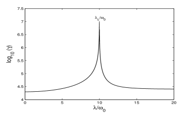
Figure 2: (Color online) The logarithm to base 10 of the PNF $\gamma$ changes with the coupling strength $\lambda$. Related parameters $N=10^{5}$, $\omega_{0}=0.05$MHz, $\omega=20$MHz correspond the experimental parameters in Ref. Baumann2010 .

Compared with the case of the normal phase, the displacement $\alpha$ due to collective excitation appears in the super-radiant phase. Figure 2 shows the PNF $\gamma$ will experience drastic change near the critical coupling point $\lambda_{c}/\omega_{0}=10$. The closer the coupling strength $\lambda$ near the critical coupling point, the larger the PNF $\gamma$. This inspires us to control the coherence decay rate of the two atomic qubits by adjusting the pumping power to change the coupling strength in the region near the critical coupling.

In the following we consider the QD amplification of the two atomic qubits induced by the QPT of the cavity-BEC system. The QD  Ollivier2001 is defined as the difference between the total correlation and the classical correlation with the expression $\mathcal{D}\left(\hat{\rho}^{AB}\right)=\mathcal{I}\left(\hat{\rho}^{A}:\hat{\rho}^{B}\right)-\mathcal{C}\left(\hat{\rho}^{AB}\right)$ with $\hat{\rho}^{A}$, $\hat{\rho}^{B}$, and $\hat{\rho}^{B}$ being the reduced density operators for subsystems $A$ and $B$, and the total density operator, respectively. The total correlation in the state $\hat{\rho}^{AB}$ is measured by quantum mutual information $\mathcal{I}\left(\hat{\rho}^{A}:\hat{\rho}^{B}\right)=S\left(\hat{\rho}^{A}\right)+S\left(\hat{\rho}^{B}\right)-S\left(\hat{\rho}^{AB}\right)$ with $S\left(\hat{\rho}\right)=-\textrm{Tr}(\hat{\rho}\log\hat{\rho})$ being the von Neumann entropy. The classical correlation between the two subsystems $A$ and $B$ is given by $C(\hat{\rho}^{AB})=S(\hat{\rho}_{A})-\min_{\{\hat{P}^{B}_{k}\}}\left[\sum_{k}p_{k}S(\hat{\rho}^{A}_{k})\right]$ where $p_{k}=\textrm{Tr}_{AB}[(\hat{I}^{A}\otimes\hat{P}^{B}_{k})\hat{\rho}^{AB}(\hat{I}^{A}\otimes\hat{P}^{B}_{k})]$ denotes the probability relating to the outcome $k$, and $\hat{I}^{A}$ denotes the identity operator for the subsystem $A$ with $\{\hat{P}^{B}_{k}\}$ being a set of projects performed locally on the subsystem $B$.

The mutual information of the state given in Eq. (5) is derived as $\mathcal{I}\left(\hat{\rho}^{A}:\hat{\rho}^{B}\right)\ =2+{\sum_{i=1}^{4}}\lambda_{i}\log\lambda_{i}$, where $\lambda_{1,2}=\frac{1}{4}(1+c_{3}\pm|\mu(t)D_{1}(t)|)$, $\lambda_{3,4}=\frac{1}{4}(1-c_{3}\pm|\nu(t)D_{2}(t)|)$ are four eigenvalues of $\hat{\rho}_{s}(t)$. And the classical correlation can be obtained as Luo2008 ; Yuan2010 $C(\hat{\rho}_{s}(t))=\overset{2}{\underset{n=1}{\sum}}\frac{1+(-1)^{n}\chi}{2}\log_{2}\left[1+(-1)^{n}\chi\right]$ with $\chi(t)=\max\left[|c_{3}|,(|\mu(t)D_{1}(t)|+|\nu(t)D_{2}(t)|)/2\right]$. Therefore, the QD can be written as

$$\mathcal{D}\left(\hat{\rho}_{s}(t)\right)\ = 2+{\sum_{i=1}^{4}}\lambda_{i}\log_{2}\lambda_{i}-C(\hat{\rho}_{s}(t)).$$ (25)

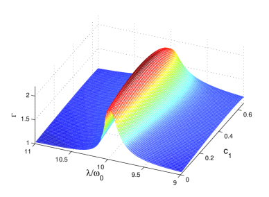
Figure 3: (Color online) The QD amplification rate as a function of the coupling strength $\lambda$ and the initial parameter $c_{1}$. Other parameters are set as $c_{3}=c_{1}/2$, $c_{2}=0$, $\omega_{0}=0.05$ MHz, $\omega=20$ MHz, $t_{f}=1/\omega_{0}$, $\delta_{1}=0.001\omega_{0}$, $\delta_{2}=0$, and $N=10^{5}$.

The QD can be amplified for some initial states such as the state parameters being set as $c_{2}=0$, $0\leq c_{1}=2c_{3}\leq 2/3$ when the qubits are in the phase decoherence environment Yuan2010 . For the present cavity-BEC environment, let the two atomic qubits enter the cavity at time $t=0$ and leave the cavity at time $t_{f}$. Then we can define the QD amplification rate as $\Gamma=\mathcal{D}(t_{f})/\mathcal{D}(0)$. In Figure 3 we have plotted the amplification rate $\Gamma$ with respect to the coupling strength $\lambda$ and the initial state parameter $c_{1}$ when $c_{3}=c_{1}/2$, $c_{2}=0$, $\omega_{0}=0.05$ MHz, $\omega=20$ MHz, $\lambda_{c}/\omega_{0}=10$, $t_{f}=1/\omega_{0}$, $\delta_{1}=0.001\omega_{0}$, $\delta_{2}=0$, and $N=10^{5}$. Figure 3 indicates that the initial QD can be amplified by the use of the cavity-BEC system through changing the QPT parameter $\lambda$. Specially, the QD amplification rate sensitively increases at the QPT point of the cavity-BEC system $\lambda=\lambda_{c}$. In this sense, the sensitive QD amplification can be understood as a quantum phenomenon induced by the QPT of the cavity-BEC system. It should be pointed out that one can control the QPT parameter $\lambda$ by changing the Rabi frequency of the pump field $\Omega_{p}$due to the relation $\lambda=\sqrt{N}g_{0}\Omega_{p}/2\Delta$.

In conclusion, we have proposed a scheme to realize the sensitive QD amplification of two atomic qubits via the cavity-BEC system through by changing the QPT parameter of the the cavity-BEC system, and and revealed the QPT mechanism of the sensitive QD amplification. We have indicated that the cavity-BEC system is equivalent to a phase decoherence environment for the two atomic qubits. Hence, it provides an artificial and controllable phase decoherence environment for quantum information processing. It should mentioned that the present scheme should be within the reach of present-day techniques since the cavity-BEC system used in the scheme has been well established in recent experiments of observing the Dicke QPT Baumann2010 . The experimental realization of the scheme proposed in the present paper deserves further investigation.

References

• (1) H. Ollivier and W. H. Zurek, Phys. Rev. Lett. 88, 017901 (2001).
• (2) L. Henderson and V. Vedral, J. Phys. A: Math. Gen. 34, 6899 (2001); V. Vedral, Phys. Rev. Lett. 90, 050401 (2003).
• (3) A. Datta, A. Shaji, and C. M. Caves, Phys. Rev. Lett. 100, 050502 (2008); B. Dakić, etal., Nature Phys. DOI:10.1038/NPHYS2377 (2012).
• (4) B. P. Lanyon, M. Barbieri, M. P. Almeida, and A. G. White, Phys. Rev. Lett. 101, 200501 (2008).
• (5) A. Datta, S. Gharibian, Phys. Rev. A 79, 042325 (2009); S. Boixo, L. Aolita, D. Cavalcanti, K. Modi and A.Winter, Int. Jour. Quant. Inf. 9, 1643 (2011).
• (6) L. Roa, J.C. Retamal, and M. Alid-Vaccarezza, Phys. Rev. Lett. 107, 080401 (2011).
• (7) B. Li, S. Fei, Z. Wang and H. Fan, Phys. Rev. A 85, 022328 (2012).
• (8) V. Madhok and A. Datta, arXiv:1204.6042.
• (9) E. Knill and R. Laflamme, Phys. Rev. Lett. 81, 5672 (1998).
• (10) J. B. Yuan, L. M. Kuang and J. Q. Liao, J. Phys. B: At .Mol. Opt. Phys. 43, 165503 (2010).
• (11) R. H. Dicke, Phys. Rev. 93, 99 (1954).
• (12) C. Emary and T. Brandes, Phys. Rev. E 67, 066203 (2003).
• (13) Sachdev S, Quantum Phase Transition, Cambridge University Press, Cambridge (1999).
• (14) K. Baumann, C. Guerlin , F. Brennecke, and T. Esslinger, Nature (London) 464, 1301 (2010); K. Baumann, R. Mottl, F. Brennecke, and T. Esslinger, Phys. Rev. Lett. 107, 140402 (2011).
• (15) K. Hepp and E. H. Lieb , Ann, Phys.(N.Y.) 76, 360 (1973);
Phys. Rev. A 8, 2517 (1973).
• (16) Y. K. Wang and F. T. Hioe, Phys. Rev. A 7, 831 (1973).
• (17) C. Emary and T. Brandes, Phys. Rev. Lett. 90, 044101 (2003).
• (18) H. T. Quan, Z. Song, X. F. Liu , P. Zanardi, and C. P. Sun, Phys. Rev. Lett. 96, 140604 (2006).
• (19) J. F. Huang, Y. Li, J. Q. Liao, L. M. Kuang, and C. P. Sun, Phys. Rev. A 80, 063829 (2009).
• (20) J. Zhang, X. Peng, N. Rajendran, and D. Suter, Phys. Rev. Lett. 100, 100501 (2008).
• (21) K. Baumann, R. Mottl, F. Brennecke, and T. Esslinger, Phys. Rev. Lett. 107, 140402 (2011).
• (22) H. Fröhlich , Phys. Rev. 79, 845 (1950).
• (23) S. Nakajima, Adv, Phys. 4, 363 (1955).
• (24) T. Holstein and H. Primakoff, Phys. Rev. 58, 1098 (1940).
• (25) S. Luo, Phys. Rev. A 77, 042303 (2008).