Revising the Halofit Model for the Nonlinear Matter Power Spectrum

Abstract

Based on a suite of state-of-the-art high-resolution $N$-body simulations, we revisit the so-called halofit model (Smith et al. 2003) as an accurate fitting formula for the nonlinear matter power spectrum. While the halofit model has been frequently used as a standard cosmological tool to predict the nonlinear matter power spectrum in a universe dominated by cold dark matter, its precision has been limited by the low-resolution of $N$-body simulations used to determine the fitting parameters, suggesting the necessity of improved fitting formula at small scales for future cosmological studies. We run high-resolution $N$-body simulations for 16 cosmological models around the Wilkinson Microwave Anisotropy Probe (WMAP) best-fit cosmological parameters (1, 3, 5, and 7 year results), including dark energy models with a constant equation of state. The simulation results are used to re-calibrate the fitting parameters of the halofit model so as to reproduce small-scale power spectra of the $N$-body simulations, while keeping the precision at large scales. The revised fitting formula provides an accurate prediction of the nonlinear matter power spectrum in a wide range of wavenumber ($k\leq 30h$ Mpc^-1) at redshifts $0\leq z\leq 10$, with $5\%$ precision for $k\leq 1\,h$ Mpc^-1 at $0\leq z\leq 10$ and $10\%$ for $1\leq k\leq 10\,h$ Mpc^-1 at $0\leq z\leq 3$. We discuss the impact of the improved halofit model on weak lensing power spectra and correlation functions, and show that the improved model better reproduces ray-tracing simulation results.

1. Introduction

The large-scale structure of the Universe has evolved under the influence of cosmic expansion and gravity, and its statistical nature contains valuable cosmological information. Among others, the power spectrum $P(k)$ is one of the most fundamental statistical quantities characterizing the large-scale structure. It has widely been used for cosmological studies, both in predicting various observable quantities and in extracting cosmological information from the observations (e.g., Peebles, 1993; Dodelson, 2003). Given growing interests in high precision cosmological observations, of particular importance is an accurate theoretical template of the power spectrum, taking account of the nonlinear gravitational evolution.

Weak lensing induced by the large-scale structure between observed galaxies and the observer provides a unique opportunity to directly probe matter inhomogeneities in the Universe. This cosmic shear signal has been measured with a high signal-to-noise ratio by current large surveys including Canada-France-Hawaii Telescope Legacy Survey (CFHTLS; Fu et al., 2008), Sloan Digital Sky Survey (SDSS; Lin et al., 2011; Huff et al., 2011), and Cosmic Evolution Survey (COSMOS; Massey et al., 2007; Schrabback et al., 2010). These surveys provided useful constraints on the cosmological parameters such as the matter density parameter $\Omega_{\rm m}$ and the amplitude of density fluctuation $\sigma_{8}$. Future surveys such as Subaru Hyper Suprime-Cam (HSC; Miyazaki et al., 2006), Dark Energy Survey (DES; The Dark Energy Survey Collaboration, 2005), and Large Synoptic Survey Telescope (LSST; LSST Science Collaborations et al., 2009) aim at measuring the cosmic shear signal with unprecedented precisions. While weak lensing probes matter fluctuations projected along the line-of-sight, one can extract the redshift evolution of the fluctuations, and hence accurate information on dark energy, using a technique called lensing tomography (e.g., Hu, 1999; Takada & Jain, 2004) or a cross-correlation with intervening objects (e.g., Oguri & Takada, 2011). However, accurate and unbiased cosmological constraints from these lensing measurements can be obtained only if we have appropriate likelihood function with given marginal distributions (Sato et al., 2010, 2011) and an accurate model of the power spectrum $P(k)$. For instance, Huterer & Takada (2005) argued that we typically need a few percent accuracy of $P(k)$ at the wavenumber $k<10h$ Mpc^-1 in order for the uncertainty of $P(k)$ not to degrade cosmological constraints in DES and LSST  (see also Eifler, 2011; Hearin et al., 2012, in which a similar conclusion is obtained).

In the linear and quasi-linear regime of density fluctuations, the power spectrum can be computed for any given initial conditions and cosmological parameters using perturbation theory (e.g., Bernardeau et al., 2002, for a review). In the nonlinear regime, however, one has to resort to cosmological $N$-body simulations to study the nonlinear gravitational evolution. $N$-body simulation results are then used to develop phenomenological halo models or fitting formulae of nonlinear gravitational clustering. For instance, Peacock & Dodds (1996) provided a fitting formula of $P(k)$ based on a scaling ansatz presented in Hamilton et al. (1991). Smith et al. (2003, hereafter S03) proposed a new model of $P(k)$, the so-called halofit model, which is based on a halo model of structure formation (e.g., Ma & Fry, 2000; Seljak, 2000; Cooray & Sheth, 2002). In this halo model, all the matter content in the Universe is assumed to be bound in dark matter halos. Then the power spectrum is decomposed into two terms, the so-called one- and two-halo terms. The one-halo term describes matter correlations within the same dark matter halo, and is determined by the density profile of each halo. On the other hand, the two-halo term arises from the correlation between two distinct halos. The one-halo term dominates at small scales, whereas the two-halo term dominate at large scales. The halofit model chose the functional form of $P(k)$ based on the halo model, but the model parameters were calibrated from $N$-body simulation results.

The halofit model by S03 is widely used to calculate the nonlinear matter power spectrum, yet it has been reported that the model fails to reproduce recent high-resolution $N$-body simulation results at small scales (e.g., Springel et al., 2005; Hilbert et al., 2009; Sato et al., 2009; Boylan-Kolchin et al., 2009; Takahashi et al., 2011b; Kiessling et al., 2011; Valageas & Nishimichi, 2011a, b; Harnois-Deraps et al., 2012; Casarini et al., 2012; Inoue & Takahashi, 2012). For instance, White & Vale (2004) first pointed out that the halofit predicts a smaller power than their numerical results at small scales. Heitmann et al. (2010) ran a suite of high-resolution simulations, called “Coyote Universe”, and showed that $P(k)$ predicted by the halofit is $\sim 5\%$ smaller than their numerical results at $k\sim 1h$ Mpc^-1. The one reason of the difference comes from the fact that the $N$-body simulations used in S03 have lower spatial resolution than latest ones. The another reason is that the halofit model in S03 is the fitting function for the Cold Dark Matter (CDM) model without baryons. An outcome of the Coyote Universe simulations is a publicly available code “cosmic emulator” to calculate the nonlinear matter power spectrum by interpolating the simulations results for 38 different cosmological models (Lawrence et al., 2010). However, their emulator is restricted to a narrow range in $k<3h{\rm Mpc}^{-1}$ and at low redshift $0\leq z\leq 1$. Also, the Hubble parameter is automatically specified in the code using the cosmic microwave background (CMB) anisotropy constraint on the distance to the last scattering surface.

In this paper, we revisit the halofit model based on state-of-the-art high-resolution $N$-body simulations in 16 cosmological models around the Wilkinson Microwave Anisotropy Probe (WMAP) best-fit cosmological parameters. We allow the dark energy equation of state $w$ to deviate from $-1$, assuming that $w$ does not evolve with redshift. The halofit model has been tested for dark energy models ($w\neq-1$) using N-body simulations  (e.g., McDonald et al., 2006; Ma, 2007; Casarini et al., 2009; Francis et al., 2009; Alimi et al., 2010; Casarini et al., 2011b). While the original halofit model in S03 contains $30$ parameters, we increase the number of parameters to $35$ in order to achieve a better fit to the simulations. The new formula we present, which is summarized in Appendix, is widely applicable in the wavenumber range of $k<30h$ Mpc^-1 and the redshift range of $0\leq z\leq 10$. Simply replacing the parameters in the original halofit model with new ones in the Appendix, an accuracy of fitting function is improved especially at small scales.

The present paper is organized as follows. In Section 2, we begin by describing the $N$-body simulations and cosmological models used for the power spectrum analysis. Combining the $N$-body results with different box sizes, we discuss in detail the convergence of power spectrum measurement over the wide range of wave number. In Section 3, we re-calibrate the halofit model, and the revised version of the halofit model, whose explicit formula is given in Appendix, is compared with our $N$-body simulations. As an important implication of revised halofit model, in Section 4, we compute weak lensing power spectra, and compare them with direct ray-tracing simulation results, particularly focusing on the small-scale behavior. Finally, Section 5 is devoted to conclusion and discussion.

2. N-body Simulations

	$\Omega_{\rm b}$	$\Omega_{\rm m}$	$h$	$\sigma_{8}$	$n_{\rm s}$	$-w$
WMAP1	$0.044$	$0.29$	$0.72$	$0.9$	$0.99$	$1$
WMAP3	$0.041$	$0.238$	$0.732$	$0.76$	$0.958$	$1$
WMAP5	$0.046$	$0.279$	$0.701$	$0.817$	$0.96$	$1$
WMAP7	$0.046$	$0.272$	$0.7$	$0.81$	$0.97$	$1$
WMAP7a	$0.046$	$0.272$	$0.7$	$0.81$	$0.97$	$0.8$
WMAP7b	$0.046$	$0.272$	$0.7$	$0.81$	$0.97$	$1.2$

Note. — Best-fit cosmological parameters in a series of WMAP papers. Here we show the baryon density $\Omega_{\rm b}$, the matter density $\Omega_{\rm m}$, the Hubble constant $h$, the amplitude of power spectrum at $8h^{-1}$ Mpc $\sigma_{8}$, the spectral index $n_{\rm s}$, and the equation of state of dark energy $w$. We assume a flat curvature ($\Omega_{\rm w}=1-\Omega_{\rm m}$).

	$\Omega_{\rm b}$	$\Omega_{\rm m}$	$h$	$\sigma_{8}$	$n_{\rm s}$	$-w$
m00	$0.0432$	$0.25$	$0.72$	$0.8$	$0.97$	$1$
m01	$0.0647$	$0.4307$	$0.5977$	$0.8161$	$0.9468$	$0.816$
m02	$0.0637$	$0.4095$	$0.5907$	$0.8548$	$0.8952$	$0.758$
m03	$0.0514$	$0.2895$	$0.6763$	$0.8484$	$0.9984$	$0.874$
m04	$0.0437$	$0.2660$	$0.7204$	$0.7$	$0.9339$	$1.087$
m05	$0.0367$	$0.2309$	$0.7669$	$0.8226$	$0.9726$	$1.242$
m06	$0.0462$	$0.3059$	$0.7040$	$0.6705$	$0.9145$	$1.223$
m07	$0.0582$	$0.3310$	$0.6189$	$0.7474$	$0.921$	$0.7$
m08	$0.0428$	$0.2780$	$0.7218$	$0.8090$	$0.9855$	$1.203$
m09	$0.0623$	$0.3707$	$0.6127$	$0.6692$	$0.979$	$0.739$

Note. — Cosmological parameters of Coyote models.

	$L(h^{-1}{\rm Mpc})$	$N_{p}^{3}$	$N_{\rm r}$	$k_{\rm Nyq}(h\,{\rm Mpc}^{-1})$	$r_{s}(h^{-1}{\rm kpc})$	$z_{\rm init}$	$z_{\rm out}$
WMAP models	$2000$	$1024^{3}$	$3$	$1.6$	$97.6$	$99$	$0,~{}0.35,~{}0.7,~{}1,~{}1.5,~{}2.2,~{}3,~{}5,~{}7,~{}10$
	$800$	$1024^{3}$	$3$	$4.0$	$39.0$	$99$	$0,~{}0.35,~{}0.7,~{}1,~{}1.5,~{}2.2,~{}3,~{}5,~{}7,~{}10$
	$320$	$1024^{3}$	$6$	$10.$	$15.6$	$99$	$0,~{}0.35,~{}0.7,~{}1,~{}1.5,~{}2.2,~{}3,~{}5,~{}7,~{}10$
Coyote models	$1000$	$1024^{3}$	$1$	$3.2$	$48.8$	$99$	$0,~{}0.35,~{}0.7,~{}1,~{}1.5,~{}2.2,~{}3,~{}5,~{}7,~{}10$
	$320$	$1024^{3}$	$1$	$10.$	$15.6$	$99$	$0,~{}0.35,~{}0.7,~{}1,~{}1.5,~{}2.2,~{}3,~{}5,~{}7,~{}10$

Note. — Model parameters of our numerical simulations for the WMAP models (upper rows) and the Coyote models (lower rows): the box size $L$, the number of particles $N_{p}^{3}$, the number of realizations $N_{\rm r}$, the Nyquist frequency $k_{\rm Nyq}=(2\pi/L)(N_{p}/2)$, the softening length $r_{s}$, the initial redshift $z_{\rm init}$ and the redshifts of the simulation outputs $z_{\rm out}$.

2.1. Power Spectrum

In this section, we describe our cosmological $N$-body simulations used in this paper. We follow the nonlinear gravitational evolution of $1024^{3}$ collisionless particles in a cubic box of side $L$. We use the public cosmological $N$-body simulation code Gadget2 which is a tree-PM code (Springel et al., 2001; Springel, 2005). We use $2048^{3}$ PM grid to follow the gravitational evolution at small scales accurately. We generate the initial conditions based on the second-order Lagrangian perturbation theory (2LPT; Crocce et al., 2006; Nishimichi et al., 2009) with the initial linear power spectrum calculated by the Code for Anisotropies in the Microwave Background (CAMB; Lewis et al., 2000). The initial redshift is set to $z_{\rm in}=99$. We store simulation results (particle positions) at various redshifts from $z=0$ to $10$. The softening length is set to $5\%$ of the mean particle separation. To calculate the power spectrum, we assign the particles on $N_{g}^{3}=1280^{3}$ grid points using the cloud-in-cells (CIC) method (Hockney & Eastwood, 1981) to obtain the density field. After performing the Fourier transform, we correct the window function of CIC by dividing each mode by the Fourier transform of the window kernel as $\tilde{\delta}_{\bf k}\rightarrow\prod_{i=x,y,z}\left[{\rm sinc}(Lk_{i}/2N_{\rm g})\right]^{-2}\times\tilde{\delta}_{\bf k}$, where $\tilde{\delta}_{\bf k}$ is the density fluctuation in Fourier space and ${\rm sinc}(x)=\sin(x)/x$ (e.g., Takahashi et al., 2009; Sato & Matsubara, 2011). In addition, to evaluate the power spectrum at small scales accurately, we fold the particle positions into a smaller box by replacing $\mathbf{x}\rightarrow\mathbf{x}\%(L/2^{n})$ where the operation $a\%b$ stands for the remainder of the division of $a$ by $b$ (e.g., Jenkins, et al., 1998; Smith et al., 2003; Valageas & Nishimichi, 2011a). This procedure leads to effectively $2^{n}$ times higher resolution. Here we adopt $n=0$, $2$, and $4$. We use the density fluctuation $\tilde{\delta}_{\bf k}$ up to half the Nyquist frequency determined by the box size $L/2^{n}$ with the grid number $N_{g}$, i.e., $1/2\times k_{\rm Nyq}$ $=(\pi/(L/2^{n}))(N_{g}/2)$, with $n=0$, $2$, and $4$. This condition corresponds to $k<6.3$, $25$, and $100h$ Mpc^-1 with $n=0$, $2$, and $4$, respectively, for the box size of $L=320h^{-1}$Mpc with $N_{g}=1280$. Finally, we compute the power spectrum

$$P(k)=\frac{1}{N_{k}}\sum_{\bf k}\left|\tilde{\delta}_{\bf k}\right|^{2},$$ (1)

where the summation over Fourier modes is done for the modes falling into the bin [$k-\Delta k/2$, $k+\Delta k/2$], and $N_{k}$ denotes the number of available Fourier modes in the bin. We do not subtract the shot noise in the measured power spectrum. Instead, we do not use $P(k)$ at small scales where the shot noise dominates (see Section 3).

2.2. Cosmological Models

In this paper, we use simulation results for 16 cosmological models. Six are taken from the results of WMAP papers and 10 are from the cosmological models adopted by the Coyote Universe. For all of the models, we assume a flat curvature ($\Omega_{\rm w}=1-\Omega_{\rm m}$, where $\Omega_{\rm w}$ is the dark energy density). The first four WMAP models, which are shown in Table 2, are the best-fit $\Lambda$CDM models of WMAP 1, 3, 5, 7 year results (Spergel et al., 2003, 2007; Komatsu et al., 2009, 2011). The other two models, WMAP7a and WMAP7b, are the same as the WMAP7 model except that we slightly change the equation of state parameter of dark energy ($w=-0.8$ and $-1.2$).

In addition, we also examine 10 models among 38 cosmological models presented in the Coyote Universe, as shown in Table 2. These models, tagged as m00 to m09, were used in a series of papers of the Coyote Universe project (Heitmann et al., 2009, 2010; Lawrence et al., 2010), in which 38 cosmological models in a parameter range of $0.120<\Omega_{\rm m}h^{2}<0.155$, $0.0215<\Omega_{\rm b}h^{2}<0.0235$, $0.85<n_{\rm s}<1.05$, $-1.30<w<-0.70$, and $0.61<\sigma_{8}<0.9$ are used to make a fitting function of the power spectrum. The models used in our paper correspond to their first 10 cosmological models. Since the cosmological parameters in Coyote models are different from the WMAP models typically by $20-30\%$, we use our simulation results for these Coyote cosmological models to check the dependence of our fitting function on cosmological parameters.

Table 2 summarizes our simulation setting, including the box size, the number of particles, the number of realizations, and the softening length, for the WMAP and Coyote models. In the WMAP models, we adopt the simulation boxes of $L=2000$, $800$, and $320h^{-1}$Mpc on a side. We prepare $3$ different random realizations for $L=2000$ and $800h^{-1}$Mpc, and $6$ realizations for $320h^{-1}$Mpc to reduce the sample variance. We combine the power spectrum $P(k)$ obtained from the different simulation boxes to cover a wide wavenumber range. The specific procedure for combining the $P(k)$ is discussed in the next subsection. We use the mean power spectrum of these realizations. The Nyquist wavenumber of the mean particle separation in the smallest box ($L=320h^{-1}$Mpc) is $k=10h$ Mpc^-1. The bin width is set linearly, $\Delta k=0.01h$ Mpc^-1, in the linear regime $k\leq 0.3h$ Mpc^-1, and logarithmically, $\Delta\log_{10}(k/h$ Mpc${}^{-1})=0.02$, in the nonlinear regime $k>0.3h$ Mpc^-1. We analyze ten outputs at redshifts $0\leq z\leq 10$, $z=0$, $0.35$, $0.7$, $1$, $1.5$, $2.2$, $3,5$, $7$, and $10$. We checked that the power spectra of our simulations agree with the results of higher resolution simulations, in which we set the finer simulation parameters for the time step, the force calculation, etc., within $2(6)\%$ for $k<10(30)h$ Mpc^-1.

In the Coyote models, we use the simulation boxes of $1000h^{-1}$Mpc and $320h^{-1}$Mpc on a side. We prepare a single realization for each of the 10 models. The Nyquist wavenumber is $k=3.2(10)h$ Mpc^-1 for $L=1000(320)h^{-1}$Mpc and we use a logarithmic bin of $\Delta\log_{10}(k/h$ Mpc${}^{-1})=0.1$. We use ten outputs at the redshifts $0\leq z\leq 10$, $z=0$, $0.35$, $0.7$, $1$, $1.5$, $2.2$, $3$, $5$, $7$, and $10$. We confirmed that our simulation results agree with the cosmic emulator results within $3\%$ for $0.1<k<3h$ Mpc^-1 at $0\leq z\leq 1$.

Finally, as a further cross check, we compare our simulation results with two high-resolution simulation results in Valageas & Nishimichi (2011a) and Takahashi et al. (2011b). In both the simulations, the same codes, Gadget-2 with 2LPT initial condition, were used. Valageas & Nishimichi (2011a) employed $2048^{3}$ particles in different box sizes of $L=4096$, $2048$, $1024$, and $512h^{-1}$Mpc. They calculated the power spectra at redshifts $z=0.35$, $1$, and $3$ in the WMAP5 model. The Nyquist wave number in the smallest box is $13h$ Mpc^-1. On the other hand, Takahashi et al. (2011b) employed $1024^{3}$ particles on the box size of $50h^{-1}$Mpc at redshift $z=0-20$. They prepared independent four realizations. The cosmological parameters are based on the WMAP 5 year result, although the values were slightly different from those of the WMAP5 model listed in Table 1. We use $14$ outputs at redshifts $z=0-10$, $z=0$, $0.35$, $0.7$, $1$, $1.5$, $2.2$, $3$, $3.4$, $4.1$, $4.7$, $5.5$, $6.4$, $7.6$, and $9.1$. The Nyquist wave number is $64h$ Mpc^-1. We use these simulation results in our analysis for only small scales, $k>10(1)h$ Mpc^-1 at $z\leq 3(>3)$, in order to check the asymptotic behavior of our fitting formula at high $k$ limit.

2.3. Accuracy of Our $N$-body Simulations

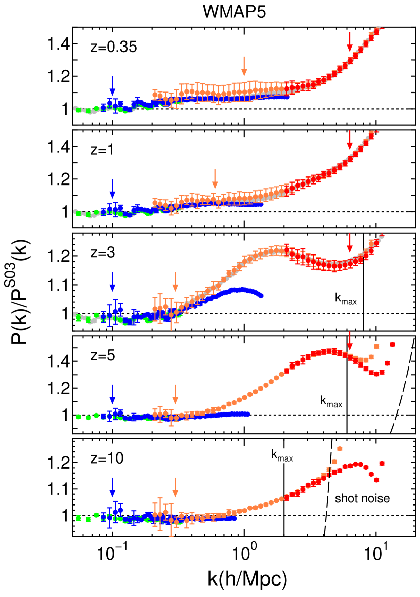
Figure 1.— Power spectra $P(k)$ from the different simulation box sizes for the WMAP5 model at redshifts $z=0.35$, $1$, $3$, $5$, and $10$. The vertical axis shows power spectra in our simulations normalized by the theoretical nonlinear matter power spectrum model from the original halofit model in S03. Green, blue, and orange symbols are simulation results from the box sizes of $L=2000$, $800$, and $320h^{-1}$Mpc, respectively. Red symbols are the same as the oranges, but including the folding method with $n=2$ (see Section 2.1). Gray symbols show simulation results from Valageas & Nishimichi (2011a). Arrows denote wavenumbers where $P(k)$ with the different box sizes are connected. Dashed curves denote the shot noise. Vertical solid lines indicate the maximum wavenumber $k_{\rm max}$ for deriving our fitting formula.

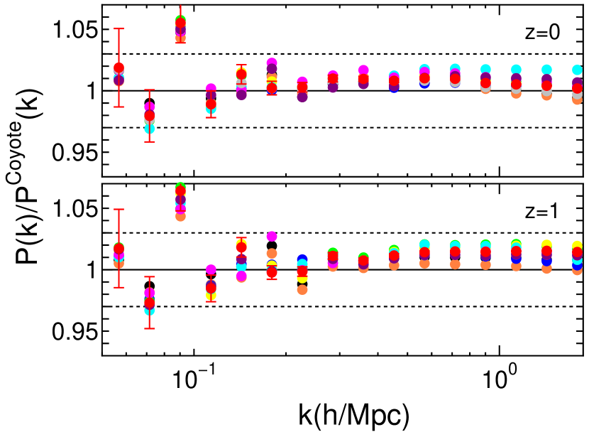
Figure 2.— Power spectra $P(k)$ from our simulations of $L=1000h^{-1}$Mpc divided by those of the Cosmic emulator for the ten Coyote models at $z=0$ (top) and $1$ (bottom). Red symbols with error bars are for the fiducial model m00. Horizontal dotted lines indicate the fractional error of $3\%$.

$z$	$k_{2000/800}$	$k_{800/320}$	$k_{\rm min}$	$k_{\rm max}$
$0,0.35$	$0.1$	$1.$	$0.02$	$30$
$0.7,1$	$0.1$	$0.6$	$0.02$	$20$
$1.5,2.2$	$0.1$	$0.4$	$0.02$	$10$
$3$	$0.1$	$0.3$	$0.02$	$8$
$5$	$0.1$	$0.3$	$0.02$	$6$
$7$	$0.1$	$0.3$	$0.02$	$3$
$10$	$0.1$	$0.3$	$0.02$	$2$

Note. — The summary of wavenumbers (in units of $h$ Mpc^-1) where the simulation results $P(k)$ with the different box sizes are connected at each redshift, $k_{2000/800}$ is for $L=2000$ and $800h^{-1}$Mpc, and $k_{800/320}$ is for $L=800$ and $320h^{-1}$Mpc. The minimum and maximum wavenumbers used in our analysis are shown by $k_{\rm min}$ and $k_{\rm max}$, respectively.

In this subsection, we compare our simulation results with previous works to check the accuracy and convergence of our $N$-body simulations. We also describe the procedure for combining the $P(k)$ from the different simulation box sizes. Figure 1 shows the power spectrum $P(k)$ of our simulations for the different box sizes for the WMAP5 model at $z=0.35$, $1$, $3$, $5$, and $10$. The vertical axis shows the measured power spectra normalized by the theoretical model of the nonlinear power spectra from the original halofit model in S03. Green, blue, and orange symbols are the results from the different box sizes of $L=2000$, $800$, and $320h^{-1}$Mpc, respectively. Red symbols are the same simulation results as plotted in the orange symbols ($L=320h^{-1}$Mpc), but using the folding method with $n=2$ in computing $P(k)$ (see Section 2.1). We plot the mean $P(k)$ with the error bars among the realizations. Gray symbols at $z=0$, $0.35$, and $1$ are the simulation results of Valageas & Nishimichi (2011a). Vertical arrows indicate the wavenumbers at which we connected the simulation results from the different box sizes. For example, we used the results from $L=800h^{-1}$Mpc between blue and the orange arrows. We connect the results of $L=800$ and $2000h^{-1}$Mpc at $k=0.1h$ Mpc^-1 for all the redshifts. This is because at the baryon acoustic oscillation (BAO) scale ($0.1h$ Mpc${}^{-1}\leq k\leq 0.3h$ Mpc^-1), the simulation results with $L=800h^{-1}$Mpc show a better agreement with those obtained from the improved perturbation theory by Taruya & Hiramatsu (2008). The initial redshift of $z_{\rm init}=99$ is high for $L=2000h^{-1}$Mpc with $1024^{3}$ particles, and hence $P(k)$ from $L=2000h^{-1}$Mpc at low redshifts is slightly smaller than the $P(k)$ from $L=800h^{-1}$Mpc. Next, in connecting the $P(k)$ from $L=800h^{-1}$ to $320h^{-1}$Mpc, we use $P(k)$ from $L=800h^{-1}$Mpc up to the wavenumber where $P(k)$ agrees with the previous high-resolution simulation results (gray symbols) at $z=0.35$, $1$, $3$. In this way, the connecting scales are determined to $k=1$, $0.6$, and $0.3h$ Mpc^-1 for $z=0.35$, $1$, and $3$, respectively. For the redshifts $z=0$, $0.7$, $1.5$, and $2.2$, we interpolate the scales derived above, and for the redshifts $z=5$, $7$, and $10$ we simply adopt the same result as that at $z=3$. The connecting scales at each redshift are summarized in Table 2.3. While these connecting scales are derived from the WMAP5 model, we also use the same connecting scales in Table 2.3 for the other cosmological models. We confirmed that the power spectra from different simulations connect smoothly at these scales in all the cosmological models studied in this paper.

Figure 2 shows the power spectrum $P(k)$ in our simulations of $L=1000h{\rm Mpc}^{-1}$ divided by that of the Cosmic emulator for the ten Coyote models at $z=0$, $1$. The colored symbols correspond to the ten Coyote models. Red symbols with error bars are for the fiducial model m00. Here the error bars show the Gaussian errors because we have only one realization for each Coyote cosmological model. As clearly seen in the Figure, our simulation results agree with the Cosmic emulator within $3\%$ for $k=0.1-2h$ Mpc^-1.

3. Halofit Model

In the halofit model, the power spectrum consists of two terms (S03):

$$\Delta^{2}(k)=\Delta_{\rm Q}^{2}(k)+\Delta_{\rm H}^{2}(k),$$ (2)

where $\Delta^{2}(k)=k^{3}P(k)/(2\pi^{2})$ is the dimensionless power spectrum. The first term is called the two-halo term that dominates at large scales, whereas the second term is referred to as the one-halo term that is important at small scales. We adopt almost the same functional form as in S03 for both the two terms in Equation (2). We use our high-resolution simulation results to re-calibrate the model parameters of the halofit formula so as to minimize the discrepancies. To do so, we employ the standard chi-squared method to find the best-fit solution:

$$\chi^{2}=\sum_{i}\sum_{k=k_{\rm min}}^{k_{\rm max}}\sum_{z=0}^{10}W(k,z)\frac{\left[P_{i,{\rm model}}(k,z)-P_{i,{\rm sim}}(k,z)\right]^{2}}{\sigma_{i}^{2}(k,z)},$$ (3)

where $P_{i,{\rm model}}$ is the model prediction, $P_{i,{\rm sim}}$ is the simulation results, and $i$ runs over the WMAP cosmological models shown in Table 2. In Eq.(3), it is better to include the correlation between the different $k$ bins at small scales for more detailed analysis (e.g., Scoccimarro et al., 1999; Takahashi et al., 2011a). However it is expensive to evaluate the covariance matrix of $P(k)$, and hence we ignore it in this paper. We note that we use only the six WMAP models in this chi-squared analysis. The remaining ten Coyote models are used to check the accuracy of our fitting formula. We simply set the variance $\sigma_{i}^{2}=P_{i,{\rm sim}}^{2}$, and the weight function is set as follows:

$$W(k,z) = 10,\quad k<0.3h\,{\rm Mpc}^{-1}~{}\&~{}0\leq z\leq 3,$$

$$= 1,\quad 0.3h\,{\rm Mpc}^{-1}\leq k<10h\,{\rm Mpc}^{-1}~{}\&~{}0\leq z\leq 3,$$

$$= 0.2,\quad k<10h\,{\rm Mpc}^{-1}~{}\&~{}3<z\leq 10,$$

$$= 0.1,\quad k\geq 10h\,{\rm Mpc}^{-1}.$$

The weight factor is chosen so that the final fitting formula gives a better accuracy at the BAO scales at low redshifts.

In (quasi-)linear regime, the error of $P(k)$ is given by the Gaussian error which is the inverse of the square root of the number of modes (e.g., Feldman et al., 1994). We consider only the wavenumber bins where the Gaussian error of $P(k)$ is less than $3\%$ for the fitting, which correspond to $k_{\rm min}=0.02h$ Mpc^-1. In nonlinear regime, the non-Gaussian error arises due to the mode coupling, but it is smaller than $5\%$ (see e.g., Takahashi et al., 2009). While the Nyquist wavenumber is $k=10h$ Mpc^-1, we sum up the wavenumber up to $k=30h$ Mpc^-1, because the nonlinear power spectrum is reliable down to scales corresponding to the softening length (e.g., Hamana et al., 2002). On the other hand, we do not use the wavenumber where the shot noise dominates the power spectrum. The maximum wave number is $k_{\rm max}=30h$ Mpc^-1 at $z=0$, $0.35$, $k_{\rm max}=20h$ Mpc^-1 at $z=0.7$ and $1$, $k_{\rm max}=10h$ Mpc^-1 at $z=1.5$ and $2.2$, and $k_{\rm max}=8$, $6$, $3$, and $2h$ Mpc^-1 at $z=3$, $5$, $7$, and $10$, respectively. The minimum and maximum wavenumbers ($k_{\rm min}$ and $k_{\rm max}$) are listed in Table 2.3. For all the WMAP models, the power spectrum at $k=k_{\rm max}$ is $10$ $(3)$ times larger than the shot noise at $z\leq 3$ ($5\leq z\leq 10$). There are $35$ free parameters in our revised halo-model ($30$ parameters in the original model). We summarize the best-fit parameters in Appendix.

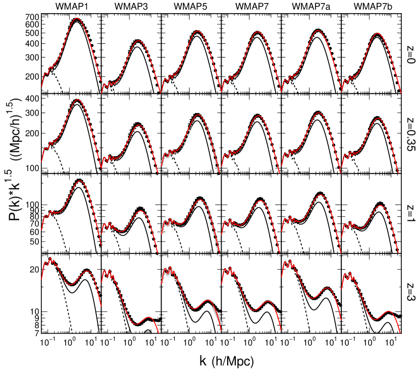
Figure 3.— Power spectra $P(k)$ for the WMAP cosmological models at $z=0$, $0.35$, $1$, and $3$. The WMAP7a,b are similar to the WMAP7 but changing the equation of state of dark energy ($w=-0.8,-1.2$). In the vertical axis, the power spectrum $P(k)$ is multiplied by the factor $k^{1.5}$ in order to show the differences between the simulation results and the theoretical models clearly. Black filled circles with the error bars plot our simulation results, and gray symbols are the results from Valageas & Nishimichi (2011a). Red solid curves show our revised halofit model (see Appendix), whereas black solid curves show the original halofit model in S03. Black dashed curves plot the linear power spectra.

Figure 3 shows the power spectra $P(k)$ as a function of the wavenumber $k$ for the WMAP1, 3, 5, 7, 7a and 7b models at redshifts $z=0$, $0.35$, $1$, and $3$. Here, to emphasize the difference between the simulation results and the theoretical models, the power spectrum $P(k)$ is multiplied by the factor $k^{1.5}$. Black circles with error bars are our simulation results, whereas gray symbols in WMAP5 are the simulation results from Valageas & Nishimichi (2011a). As seen in the Figure, our simulation results agree with the results in Valageas & Nishimichi (2011a) very well. Red curves show our fitting function, which are significantly better than the original halofit model in S03 shown by black curves. As clearly seen in the Figure, the original halofit model grossly underestimates the power spectra at smaller scales ($k\gtrsim 0.1h$ Mpc^-1). Our model agrees with the simulation results very well down to small scales for all the cosmological models. The agreement of our fitting formula with simulations is better than $8\%$ at $k<10h$ Mpc^-1 for the WMAP cosmological models in the redshift range of $0\leq z\leq 3$. For all the WMAP cosmological models at $k_{\rm min}\leq k\leq k_{\rm max}$, the rms deviation of our best-fit model from the simulation results is $1.7\%$ at $0\leq z\leq 10$.

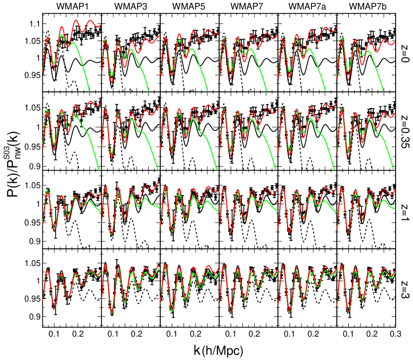
Figure 4.— Similar to Figure 3, but focusing on the BAO scale of $0.05h$ Mpc${}^{-1}<k<0.3h$ Mpc^-1. The vertical axis show $P(k)$ normalized by the smooth nonlinear power spectrum $P_{\rm nw}^{\rm S03}(k)$ which is calculated by using a no-wiggle fitting formula of Eisenstein & Hu (1998) and the original halofit model in S03 for the nonlinear correction. Again, red solid curves show our revised halofit model, whereas black solid curves show the original halofit model in S03. Green curves show the prediction by the closure theory which is a higher-order perturbation theory by Taruya & Hiramatsu (2008). Dashed curves show the linear power spectra.

Figure 4 shows the same results as in Figure 3, but we focus on the results at the BAO scale of $0.05h$ Mpc${}^{-1}<k<0.3h$ Mpc^-1. In the vertical axis, the power spectrum is normalized by the smooth nonlinear power spectrum $P_{\rm nw}^{\rm S03}(k)$, which is calculated by using a no-wiggle fitting formula of Eisenstein & Hu (1998) with nonlinear corrections computed by the original halofit model in S03. Green curves show theoretical predictions obtained from the improved perturbation theory called closure theory, which efficiently resumms a class of infinite series of higher-order perturbative corrections (Taruya & Hiramatsu, 2008; Hiramatsu & Taruya, 2009; Taruya et al., 2009). These predictions include the corrections at the 2-loop order based on the Born approximation. The Figure indicates that our model agrees with the simulation results better than S03 especially at low redshifts. However, the closure theory shows even better agreements in the quasi-linear regime. In the BAO scales, our fitting formula reproduces simulation results within $4.6\%$ for the WMAP models at $0\leq z\leq 3$.

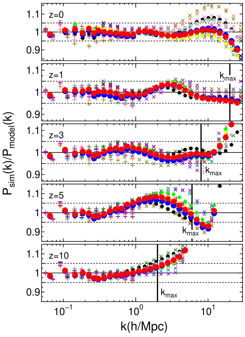
Figure 5.— Our simulation results of the power spectrum $P_{\rm sim}(k)$ divided by our improved fitting formula $P_{\rm model}(k)$ (see Appendix) for all the cosmological models at $z=0$, $1$, $3$, $5$, and $10$ (from top to bottom). Filled circles show results for the six WMAP models, whereas plus and cross symbols are for the ten Coyote models. Blue and red big circles are WMAP5 and WMAP7. Black, green, gray and yellow circles are results for the WMAP1, 3, 7a and 7b models, respectively. Horizontal dotted lines indicates the relative error of $5\%$.

Figure 5 shows ratios of the measured power spectra in our simulations to the revised fitting formula, $P_{\rm sim}(k)/P_{\rm model}(k)$, for all the cosmological models at $z=0$, $1$, $3$, $5$, and $10$. Filled circles shows results for the six WMAP models, whereas plus and cross symbols are for the ten Coyote models. The plus and cross symbols are the results from larger (smaller) box sizes $L=1000(320)h^{-1}$Mpc and are shown only for larger (smaller) scales of $k\leq 1(\geq 0.3)h$ Mpc^-1. The horizontal dotted lines show the errors of $5\%$. Vertical solid lines at $z=1$, $3$, $5$, and $10$ indicate the maximum wavenumber $k_{\rm max}$ in the chi-squared calculation in Equation (3). Note that $k_{\rm max}=30h$ Mpc^-1 at $z=0$. As seen in the Figure, relative errors are typically less than $5(10)\%$ at $z\leq 3(10)$ for all the cosmological models. Although we did not include the Coyote models in our fitting, our fitting formula reproduces simulation results for the Coyote models very well, with the errors less than $8\%$ for $k\leq 1h$ Mpc^-1 at $z=0-10$, and $13\%$ for $k\leq 10h$ Mpc^-1 at $z=0-3$. Our fiducial models (WMAP5 and 7) show better agreement, while the other models involves slightly larger errors. At $z=0$, the cosmological models with dark energy ($w\neq-1$) and with high $\sigma_{8}$ (WMAP1) show larger errors. The cosmological models with large (small) equation of state $w$ show the larger (smaller) simulation results $P_{\rm sim}(k)$ than our fitting model. For example, for the Coyote m01 ($w=-0.816$) and m02 ($w=-0.758$) models, shown as the brown and orange crosses, the simulation results are over $10\%$ larger than our best fitting model for $k\simeq 10h{\rm Mpc}^{-1}$ at $z=0$. At higher redshifts $z\geq 3$, the increase of the ratio at high $k$ are due to the shot noise. At high $z$, the errors depend mainly on the spectral index $n_{s}$ since cosmological models converge to the Einstein de-Sitter model. The models with the steep (shallow) spectral index shows the large (small) ratio at small scales $k>1h$ Mpc^-1.

Peacock also provided an improved halofit model which gives simply factor two times larger power than the original model for small scales $k>10h{\rm Mpc}^{-1}$ (see his homepage). But, his model predicts a smaler power than our simulation results at quasi-linear scale ($k=0.1-1h\,{\rm Mpc}^{-1}$). As clearly seen in the figure 1, the ratio of the simulation results to the halofit in S03 is not two for $k>10h{\rm Mpc}^{-1}$. Rather, the ratio is functions of the redshift, the wavenumber and the cosmological parameters.

4. Implications for Weak Lensing Predictions

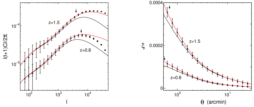
Figure 6.— Convergence power spectra (left) and correlation functions (right) at the source redshifts of $z_{s}=0.8$ and $1.5$. Red curves show theoretical predictions using our revised halofit model, and black curves show those from the original halofit model in S03. Filled circles with error bars plot ray-tracing simulation results from Sato et al. (2009, 2011). Vertical arrows show the scale down to which the ray-tracing simulation results are accurate within $5\%$. Error bars are for a $5\times 5$ ${\rm deg}^{2}$ survey, and scale as the inverse square root of the field-of-view.

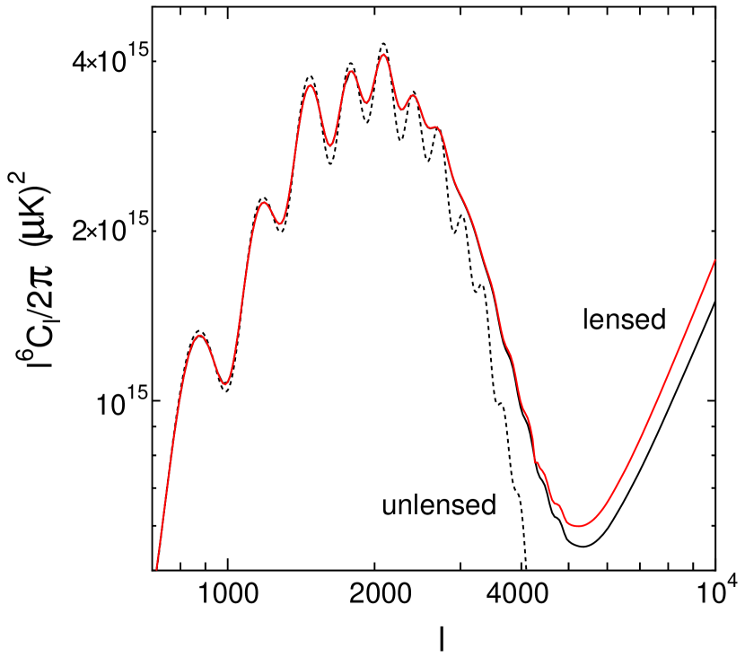
Figure 7.— The lensed CMB temperature power spectrum. The red curve shows the prediction of the our revised halofit model, while the black curve is that of the original halofit model in S03. The dashed curve shows the unlensed temperature power spectrum. Note that we plot the temperature power spectrum multiplied by $\ell^{6}$, i.e., $\ell^{6}C_{\ell}/(2\pi)$, not the usual convention of $\ell(\ell+1)C_{\ell}/(2\pi)$.

In this section, we study how the revised model of the matter nonlinear power spectrum affects weak lensing observables. Specifically, we calculate the convergence power spectra, correlation functions, and the CMB lensing using the new fitting formula that is summarized in Appendix. We compare results based on our fitting formula with those from the original halofit model in S03 as well as the direct ray-tracing simulation results.

Images of distant galaxies are distorted by gravitational lensing due to intervening matter fluctuations (e.g., Bartelmann & Schneider, 2001; Munshi et al., 2008, for a review). The image deformation is characterized by the lensing convergence $\kappa$ and shear $\gamma$. The convergence field is expressed as the integration of a weighted three-dimensional density fluctuations along the line-of-sight. Hence, the convergence power spectrum $C_{\ell}$ can be expressed as a projection of the matter power spectrum weighted with the radial lensing kernel along the line-of-sight:

$$C_{\ell}=\int_{0}^{z_{s}}dz\,W(z,z_{s})P\left(k=\frac{\ell}{\chi(z)};z\right),$$ (4)

where $W(z,z_{s})$ is a weight function.

Figure 6 shows the convergence power spectra and correlation functions in the WMAP3 model at source redshifts $z_{s}=0.8$ and $1.5$. In both panels, red solid curves show the prediction using our revised model of the power spectrum, and black solid curves show that from the original halofit model in S03. Filled circles with error bars plot direct ray-tracing simulation results obtained in Sato et al. (2009, 2011). They used a standard ray-tracing method using code “RAYTRIX” (Hamana & Mellier, 2001). With the $256^{3}$ particles in the rectangular box of $240$ and $480h^{-1}$Mpc on each side, they prepared $1000$ convergence and shear maps in the field of view $5\times 5$ ${\rm deg}^{2}$. The mean and error shown in Figure 6 are estimated from the $1000$ realizations. Note that the size of error bars is inversely proportional to the square root of the sky coverage. For example, the Subaru HSC wide survey will observe $\sim 1500$ deg², which suggests that expected error bars are $\sim 8$ times smaller than those plotted here. Vertical arrows indicate the multipole below which their simulations are consistent with higher resolution simulations ($512^{3}$ particles) within $5\%$. The Figure indicates that our model predictions agree with the simulation results much better than those of the original halofit model. This suggests that the use of the improved fitting formula as presented in this paper is essential to extract cosmological information from future high-resolution weak lensing measurements.

We also consider the weak lensing effect on the CMB temperature anisotropy. Gravitational lensing by foreground matter distributions is known to affect the light path of CMB photons coming from the last scattering surface (e.g., Lewis & Challinor, 2006). As a result, the spatial pattern of CMB temperature fluctuations is distorted, which leads to the modification of the temperature power spectrum. Since the lensing deflection angle is typically a few arcmin, the temperature power spectrum shape is significantly modified at smaller scales of $\ell\gtrsim 1000$. Figure 7 shows the predicted lensed CMB temperature power spectrum. We use the CAMB code to compute the unlensed (primordial) CMB power spectrum, which is plotted by the dashed curve. The red solid curve is the lensed power spectrum using our revised fitting formula, while the black solid curve is the one derived from the original halofit model in S03. The fitting formula of the matter power spectrum is used to calculate the power spectrum of the deflection angle by the foreground matter distribution. We find that our model enhances the power at small scales $l>4000$ by $\sim 10\%$.

5. Conclusion and Discussion

The halofit model presented in S03 has widely been used as a standard cosmological tool to predict the nonlinear matter power spectrum. However, it has been argued that the halofit model fails to reproduce recent high-resolution simulation results such that it underestimates the power spectrum by a few ten percent at small scales ($k\gtrsim 0.1h$ Mpc^-1). The difference is crucial for analysis of upcoming weak lensing surveys such as Subaru HSC survey, DES, and LSST. In this paper, we have revisited the halofit model using the high resolution simulations for the $16$ cosmological models around the WMAP best-fit cosmological parameters, including the variation in the equation of state of dark energy. The revised fitting formula can reproduce the simulation results very well in the range of $k<30h$ Mpc^-1 and $0\leq z\leq 10$. Our new fitting formula is summarized in Appendix, which can easily be updated from the original halofit model by simply replacing parameters in original model with new values as well as adding a few terms. Our revised halofit is now implemented in current version of CAMB (Oct. 2012), and hence one can easily calculate the nonlinear power spectrum $P(k)$ and the resulting weak lensing power spectra $C_{\ell}$ and lensed CMB power spectrum $C_{\ell}$ in our revised halofit model using CAMB.

We comment on effects of baryon cooling and massive neutrinos, both of which affect $P(k)$ at small scales. The baryon cooling would enhance the power at small scales by some ten percent at $k=10h$ Mpc^-1 and the enhancement becomes more significant for smaller scales (e.g., Jing et al., 2006; Rudd et al., 2008; Casarini et al., 2011a; van Daalen et al., 2011; Casarini et al., 2012). However, the reliability of simulation results strongly relies on galaxy formation models they adopted. For example, van Daalen et al. (2011) showed that the AGN feedback can decrease the power spectrum by $>10\%$ at $k>1h$ Mpc^-1. The massive neutrinos also suppress the growth of density fluctuation below the so-called freestreaming scales (e.g., Brandbyge & Hannestad, 2009; Bird et al., 2012). The power spectrum is suppressed by a few ten percent at small scales of $k\simeq 0.1h$ Mpc^-1, depending on the total mass of neutrinos. Even though these effects can modify the small-scale nonlinear matter power spectrum, an accurate knowledge of the original (dark matter only) nonlinear power spectra as presented in this paper is still important as an ingredient for building models of more realistic nonlinear power spectra which take these effects into account.

Finally, while we have improved the fitting formula using the simulations, there are also several attempts to improve the halo model analytically. For instance, combining the perturbation theory at large scales with the halo model at small scales, Valageas & Nishimichi (2011a, b) and Valageas et al. (2012a, b) presented an improved halo model. On smaller scales, Giocoli et al. (2010) provided a prediction of the power spectrum using the halo model including the effect of substructure in the individual halo. These models also reproduce the simulation results well and are consistent with our fitting formula.

Appendix A Functional Form of the Revised Halofit Model

In this Appendix, we provide the functional form of the revised halofit model. The nonlinear power spectrum, $\Delta^{2}(k)=k^{3}P(k)/(2\pi^{2})$, consist of one- and two-halo terms:

$$\Delta^{2}(k)=\Delta_{\rm Q}^{2}(k)+\Delta_{\rm H}^{2}(k).$$ (A1)

The two-halo term $\Delta_{\rm Q}^{2}(k)$ is given by,

$$\Delta_{\rm Q}^{2}(k)=\Delta_{\rm L}^{2}(k)\left[\frac{\left\{1+\Delta_{\rm L}^{2}(k)\right\}^{\beta_{\rm n}}}{1+\alpha_{\rm n}\Delta_{\rm L}^{2}(k)}\right]e^{-f(y)},$$ (A2)

where $\Delta_{\rm L}^{2}=k^{3}P_{\rm L}(k)/(2\pi^{2})$, $f(y)=y/4+y^{2}/8$, and $P_{\rm L}(k)$ is the linear power spectrum. The one-halo term $\Delta_{\rm H}^{2}(k)$ is written as

$$\Delta_{\rm H}^{2}(k)=\frac{\Delta_{\rm H}^{\prime 2}(k)}{1+\mu_{\rm n}y^{-1}+\nu_{\rm n}y^{-2}}~{}~{}{\rm with}~{}~{}\Delta_{\rm H}^{\prime 2}(k)=\frac{a_{\rm n}y^{3f_{1}(\Omega_{\rm m})}}{1+b_{\rm n}y^{f_{2}(\Omega_{\rm m})}+\left[c_{\rm n}f_{3}(\Omega_{\rm m})y\right]^{3-\gamma_{\rm n}}},$$ (A3)

where $y$ is the dimensionless wavenumber, $y=k/k_{\sigma}$. The nonlinear scale $k_{\sigma}^{-1}$ is defined by

$$\sigma^{2}(k_{\sigma}^{-1})=1~{}~{}{\rm with}~{}~{}\sigma^{2}(R)=\int d\ln k~{}\Delta_{\rm L}^{2}(k)e^{-k^{2}R^{2}}.$$ (A4)

The effective spectral index $n_{\rm eff}$ and the curvature $C$ are defined as

$$n_{\rm eff}+3=-\left.\frac{d\ln\sigma^{2}(R)}{d\ln R}\right|_{\sigma=1},~{}~{}C=-\left.\frac{d^{2}\ln\sigma^{2}(R)}{d\ln R^{2}}\right|_{\sigma=1},$$ (A5)

The parameters $a_{\rm n}$, $b_{\rm n}$, $c_{\rm n}$, $\gamma_{\rm n}$, $\alpha_{\rm n}$, $\beta_{\rm n}$, $\mu_{\rm n}$, and $\nu_{\rm n}$ in Equations (A2) and (A3) are given by polynomials as a functions of $n_{\rm eff}$ and $C$. We determine the coefficients in the polynomials by fitting the model to our simulation results, as described in Section 3. The best-fit parameters are

$$\log_{10}a_{\rm n}=1.5222+2.8553n_{\rm eff}+2.3706n_{\rm eff}^{2}+0.9903n_{\rm eff}^{3}+0.2250n_{\rm eff}^{4}-0.6038C$$

$$\hskip 142.26378pt+0.1749\Omega_{\rm w}(z)\left(1+w\right),$$ (A6)

$$\log_{10}b_{\rm n}=-0.5642+0.5864n_{\rm eff}+0.5716n_{\rm eff}^{2}-1.5474C+0.2279\Omega_{\rm w}(z)\left(1+w\right),$$ (A7)

$$\log_{10}c_{\rm n}=0.3698+2.0404n_{\rm eff}+0.8161n_{\rm eff}^{2}+0.5869C,$$ (A8)

$$\gamma_{\rm n}=0.1971-0.0843n_{\rm eff}+0.8460C,$$ (A9)

$$\alpha_{\rm n}=\left|6.0835+1.3373n_{\rm eff}-0.1959n_{\rm eff}^{2}-5.5274C\right|,$$ (A10)

$$\beta_{\rm n}=2.0379-0.7354n_{\rm eff}+0.3157n_{\rm eff}^{2}+1.2490n_{\rm eff}^{3}+0.3980n_{\rm eff}^{4}-0.1682C,$$ (A11)

$$\mu_{\rm n}=0,$$ (A12)

$$\log_{10}\nu_{\rm n}=5.2105+3.6902n_{\rm eff},$$ (A13)

where $\Omega_{\rm w}(z)$ is the dark energy density parameter at redshift $z$. The last terms in Equations (A6) and (A7) represent small correction terms for dark energy $w\neq-1$. We use the absolute value of $\alpha_{\rm n}$ in Equation (A10) to avoid divergence in the two-halo term (Equation (A2)). Finally, $f_{1,2,3}(\Omega)$ in Equation (A3) are the same as in S03

$$f_{1}(\Omega_{\rm m})=\Omega_{\rm m}^{-0.0307},~{}f_{2}(\Omega_{\rm m})=\Omega_{\rm m}^{-0.0585},~{}f_{3}(\Omega_{\rm m})=\Omega_{\rm m}^{0.0743},$$ (A14)

where $\Omega_{\rm m}$ is the matter density parameter at redshift $z$.

In summary, one can easily revise the original halofit model in S03 by replacing the parameters $a_{\rm n}$, $b_{\rm n}$, $c_{\rm n}$, $\gamma_{\rm n}$, $\alpha_{\rm n}$, $\beta_{\rm n}$, $\mu_{\rm n}$, and $\nu_{\rm n}$ to those listed in Equations (A6)-(A13).

References

- Alimi et al. (2010) Alimi, J.-M., Füzfa, A., Boucher, V., et al. 2010, MNRAS, 401, 775
- Bartelmann & Schneider (2001) Bartelmann, M., & Schneider, P. 2001, Phys. Rep., 340, 291
- Bernardeau et al. (2002) Bernardeau, F., Colombi, S., Gaztañaga, E., & Scoccimarro, R. 2002, Phys. Rep., 367, 1
- Bird et al. (2012) Bird, S., Viel, M., & Haehnelt, M. G. 2012, MNRAS, 420, 2551
- Boylan-Kolchin et al. (2009) Boylan-Kolchin, M., Springel, V., White, S. D. M., Jenkins, A., & Lemson, G. 2009, MNRAS, 398, 1150
- Brandbyge & Hannestad (2009) Brandbyge, J., & Hannestad, S. 2009, JCAP, 5, 2
- Casarini et al. (2009) Casarini, L., Macciò, A. V., Bonometto, S. A. 2009, JCAP, 03, 014
- Casarini et al. (2011a) Casarini, L., Macciò, A. V., Bonometto, S. A., & Stinson, G. S. 2011, MNRAS, 412, 911
- Casarini et al. (2011b) Casarini, L., La Vacca, G., Amendola, L., et al. 2011, JCAP, 03, 026
- Casarini et al. (2012) Casarini, L., Bonometto, S. A., Borgani, S., et al. 2012, A&A, 542, 126
- Cooray & Sheth (2002) Cooray, A., & Sheth, R. 2002, Phys. Rep., 372, 1
- Crocce et al. (2006) Crocce, M., Pueblas, S., & Scoccimarro, R. 2006, MNRAS, 373, 369
- Dodelson (2003) Dodelson, S. 2003, Modern Cosmology, Academic Press
- Eifler (2011) Eifler, T. 2011, MNRAS, 418, 536
- Eisenstein & Hu (1998) Eisenstein, D. J., & Hu, W. 1998, ApJ, 496, 605
- Feldman et al. (1994) Feldman, H. A., Kaiser, N., & Peacock, J. A. 1994, ApJ, 426, 23
- Francis et al. (2009) Francis, M. J., Lewis, G. F. & Linder, E.V. 2009, MNRAS, 394, 605
- Fu et al. (2008) Fu, L., Semboloni, E., Hoekstra, H., et al. 2008, A&A, 479, 9
- Giocoli et al. (2010) Giocoli, C., Bartelmann, M., Sheth, R. K., & Cacciato, M. 2010, MNRAS, 408, 300
- Hamana & Mellier (2001) Hamana, T., & Mellier, Y. 2001, MNRAS, 327, 169
- Hamana et al. (2002) Hamana, T., Yoshida, N., & Suto, Y. 2002, ApJ, 568, 455
- Hamilton et al. (1991) Hamilton, A. J. S., Kumar, P., Lu, E., & Matthews, A. 1991, ApJ, 374, L1
- Harnois-Deraps et al. (2012) Harnois-Deraps, J., Vafaei, S., & van Waerbeke, L. 2012, submitted to MNRAS, arXiv:1202.2332
- Hearin et al. (2012) Hearin, A. P., Zentner, A. R. & Ma, Z. 2012, JCAP, 04, 034
- Heitmann et al. (2009) Heitmann, K., Higdon, D., White, M., et al. 2009, ApJ, 705, 156
- Heitmann et al. (2010) Heitmann, K., White, M., Wagner, C., Habib, S., & Higdon, D. 2010, ApJ, 715, 104
- Hilbert et al. (2009) Hilbert, S., Hartlap, J., White, S. D. M., & Schneider, P. 2009 A&A, 499, 31
- Hiramatsu & Taruya (2009) Hiramatsu, T., & Taruya, A. 2009, Phys. Rev. D, 79, 103526
- Hockney & Eastwood (1981) Hockney, R. E. & Eastwood, J.W., 1981, Computer Simulation Using Particles (New York: McGraw-Hill)
- Hu (1999) Hu, W. 1999, ApJ, 522, L21
- Huff et al. (2011) Huff, E. M., et al. 2011, submitted to MNRAS, arXiv:1112.3143
- Huterer & Takada (2005) Huterer, D., & Takada, M. 2005, Astroparticle Physics, 23, 369
- Inoue & Takahashi (2012) Inoue, K.T. & Takahashi, R. 2012, MNRAS, 426, 2978
- Jenkins, et al. (1998) Jenkins, A., Frenk, C. S., Pearce, F. R., et al. 1998, ApJ, 499, 20
- Jing et al. (2006) Jing, Y. P., Zhang, P., Lin, W. P., Gao, L., & Springel, V. 2006, ApJ, 640, L119
- Kiessling et al. (2011) Kiessling, A., Heavens, A. F., Taylor, A. N., & Joachimi, B. 2011, MNRAS, 414, 2235
- Komatsu et al. (2009) Komatsu, E., Dunkley, J., Nolta, M. R., et al. 2009, ApJS, 180, 330
- Komatsu et al. (2011) Komatsu, E., Smith, K. M., Dunkley, J., et al. 2011, ApJS, 192, 18
- Lawrence et al. (2010) Lawrence, E., Heitmann, K., White, M., et al. 2010, ApJ, 713, 1322
- Lewis et al. (2000) Lewis, A., Challinor, A., & Lasenby, A. 2000, ApJ, 538, 473
- Lewis & Challinor (2006) Lewis, A., & Challinor, A. 2006, Phys. Rep., 429, 1
- Lin et al. (2011) Lin, H., et al. 2011, submitted to ApJ, arXiv:1111.6622
- LSST Science Collaborations et al. (2009) LSST Science Collaborations, et al. 2009, arXiv:0912.0201
- Ma & Fry (2000) Ma, C.-P. & Fry, J.N. 2000, ApJ, 543, 503
- Ma (2007) Ma, Z. 2007, ApJ, 665, 887
- Massey et al. (2007) Massey, R., Rhodes, J., Leauthaud, A., et al. 2007, ApJS, 172, 239
- McDonald et al. (2006) McDonald, P., Trac, H., & Contaldi, C. 2006, MNRAS, 366, 547
- Miyazaki et al. (2006) Miyazaki, S., et al. 2006, Proc. SPIE, 6269, 9
- Munshi et al. (2008) Munshi, D., Valageas, P., van Waerbeke, L., & Heavens, A. 2008, Phys. Rep., 462, 67
- Nishimichi et al. (2009) Nishimichi, T., Shirata, A., Taruya, A., et al. 2009, PASJ, 61, 321
- Oguri & Takada (2011) Oguri, M., & Takada, M. 2011, Phys. Rev. D, 83, 023008
- Peacock & Dodds (1996) Peacock, J. A., & Dodds, S. J. 1996, MNRAS, 280, L19
- Peebles (1993) Peebles, P. J. E. 1993, Principles of Physical Cosmology, Princeton University Press
- Rudd et al. (2008) Rudd, D. H., Zentner, A. R., & Kravtsov, A. V. 2008, ApJ, 672, 19
- Sato et al. (2009) Sato, M., Hamana, T., Takahashi, R., et al. 2009, ApJ, 701, 945
- Sato et al. (2010) Sato, M., Ichiki, K., & Takeuchi, T. T. 2010, Physical Review Letters, 105, 251301
- Sato et al. (2011) Sato, M., Ichiki, K., & Takeuchi, T. T. 2011, Phys. Rev. D, 83, 023501
- Sato & Matsubara (2011) Sato, M., & Matsubara, T. 2011, Phys. Rev. D, 84, 043501
- Sato et al. (2011) Sato, M., Takada, M., Hamana, T., & Matsubara, T. 2011, ApJ, 734, 76
- Schrabback et al. (2010) Schrabback, T., Hartlap, J., Joachimi, B., et al. 2010, A&A, 516, A63
- Scoccimarro et al. (1999) Scoccimarro, R., Zaldarriaga, M., & Hui, L. 1999, ApJ, 527, 1
- Seljak (2000) Seljak, U. 2000, MNRAS, 318, 203
- Smith et al. (2003) Smith, R. E., Peacock, J. A., Jenkins, A., et al. 2003, MNRAS, 341, 1311 (S03)
- Spergel et al. (2003) Spergel, D. N., Verde, L., Peiris, H. V., et al. 2003, ApJS, 148, 175
- Spergel et al. (2007) Spergel, D. N., Bean, R., Doré, O., et al. 2007, ApJS, 170, 377
- Springel et al. (2001) Springel, V., Yoshida, N., & White, S. D. M. 2001, New Astron., 6, 79
- Springel (2005) Springel, V. 2005, MNRAS, 364, 1105
- Springel et al. (2005) Springel, V., White, S. D. M., Jenkins, A., et al. 2005, Nature, 435, 629
- Takada & Jain (2004) Takada, M., & Jain, B. 2004, MNRAS, 348, 897
- Takahashi et al. (2009) Takahashi, R., Yoshida, N., Takada, M., et al. 2009, ApJ, 700, 479
- Takahashi et al. (2011a) Takahashi, R., Yoshida, N., Takada, M., et al. 2011, ApJ, 726, 7
- Takahashi et al. (2011b) Takahashi, R., Oguri, M., Sato, M., & Hamana, T. 2011, ApJ, 742, 15
- Taruya & Hiramatsu (2008) Taruya, A., & Hiramatsu, T. 2008, ApJ, 674, 617
- Taruya et al. (2009) Taruya, A., Nishimichi, T., Saito, S., & Hiramatsu, T. 2009, Phys. Rev. D, 80, 123503
- The Dark Energy Survey Collaboration (2005) The Dark Energy Survey Collaboration 2005, arXiv:astro-ph/0510346
- Valageas & Nishimichi (2011a) Valageas, P., & Nishimichi, T. 2011, A&A, 527, A87
- Valageas & Nishimichi (2011b) Valageas, P., & Nishimichi, T. 2011, A&A, 532, A4
- Valageas et al. (2012a) Valageas, P., Sato, M., & Nishimichi, T. 2012, A&A, 541, A161
- Valageas et al. (2012b) Valageas, P., Sato, M., & Nishimichi, T. 2012, A&A, 541, A162
- van Daalen et al. (2011) van Daalen, M. P., Schaye, J., Booth, C. M., & Dalla Vecchia, C. 2011, MNRAS, 415, 3649
- White & Vale (2004) White, M., & Vale, C. 2004, Astroparticle Physics, 22, 19