Magnetic Dipole and Electric Quadrupole Transitions in the Trivalent Lanthanide Series: Calculated Emission Rates and Oscillator Strengths

Abstract

Given growing interest in optical-frequency magnetic dipole transitions, we use intermediate coupling calculations to identify strong magnetic dipole emission lines that are well suited for experimental study. The energy levels for all trivalent lanthanide ions in the $4f^{\text{n}}$ configuration are calculated using a detailed free ion Hamiltonian, including electrostatic and spin-orbit terms as well as two-body, three-body, spin-spin, spin-other-orbit, and electrostatically correlated spin-orbit interactions. These free ion energy levels and eigenstates are then used to calculate the oscillator strengths for all ground-state magnetic dipole absorption lines and the spontaneous emission rates for all magnetic dipole emission lines including transitions between excited states. A large number of strong magnetic dipole transitions are predicted throughout the visible and near-infrared spectrum, including many at longer wavelengths that would be ideal for experimental investigation of magnetic light-matter interactions with optical metamaterials and plasmonic antennas.

I Introduction

The natural optical-frequency magnetic dipole (MD) transitions in trivalent lanthanide ions have attracted considerable attention in recent years for their ability to interact with the magnetic component of light.Thommen and Mandel (2006); Noginova et al. (2008, 2009); Yang et al. (2009); Ni et al. (2011); Taminiau et al. (2012); Karaveli and Zia (2010, 2011); Feng et al. (2011); Grosjean et al. (2011); Sheikholeslami et al. (2011) Although most light-matter interactions are mediated by electric fields through electric dipole (ED) transitions, the intra-$4f^{\text{n}}$ optical transitions of the lanthanide series are well-known to include strong MD contributions. Freed and Weissman (1941); Drexhage (1974); Kunz and Lukosz (1980); Rikken and Kessener (1995); Zampedri et al. (2007); Duan et al. (2011); Weber (1967, 1968); Carnall et al. (1968) Spurred by recent advances in optical metamaterials and nanophotonics, researchers have proposed a variety of ways to leverage natural MD transitions, e.g. as the building blocks for homogeneous negative index materials Thommen and Mandel (2006) and as probes for the local magnetic field. Noginova et al. (2008, 2009); Yang et al. (2009); Ni et al. (2011); Taminiau et al. (2012) Experimental studies have also demonstrated how the competition between ED and MD processes can be used to achieve strong enhancement of MD emission Karaveli and Zia (2010) and to broadly tune emission spectra.Karaveli and Zia (2011) Numerical investigations have shown how the enhanced magnetic field in and around metal and dielectric nanostructures can promote MD transitions, Klimov (2002); Klimov and Ducloy (2000); Feng et al. (2011); Grosjean et al. (2011); Sheikholeslami et al. (2011); Rolly et al. (2012); Schmidt et al. (2012) illustrating how near-field enhancements can modify optical selection rules to promote higher order (ED forbidden) optical processes. Zurita-Sánchez and Novotny (2002a, b); Klimov and Ketokhov (2005); Klimov and Ducloy (2005); Tojo et al. (2004, 2005); Tojo and Hasuo (2005); Yang et al. (2009); Andersen et al. (2011); Kern and Martin (2012); Klimov et al. (2012); Filter et al. (2012)

Recent studies have focused primarily on the visible ${}^{5}D_{0}\rightarrow{}^{7}F_{1}$ MD transition in trivalent Europium (Eu³⁺) and the near-infrared ${}^{4}I_{13/2}\rightarrow{}^{4}I_{15/2}$ MD transition in trivalent Erbium (Er³⁺).Thommen and Mandel (2006); Noginova et al. (2008, 2009); Ni et al. (2011); Taminiau et al. (2012); Karaveli and Zia (2010, 2011) The emphasis on these transitions is not surprising, because they have a long history of scientific and technological importance. The ${}^{5}D_{0}\rightarrow{}^{7}F_{1}$ MD transition in Eu³⁺ near $588$ nm was first characterized in 1941Freed and Weissman (1941) and subsequently used by Drexhage,Drexhage (1974) Kunz and LukoszKunz and Lukosz (1980) in their authoritative studies of modified spontaneous emission. More recently, spontaneous emission from the Eu³⁺ MD transition has served as a reference standard in studies of local field effects Rikken and Kessener (1995); Zampedri et al. (2007); Duan et al. (2011) and ligand environments.Werts et al. (2002) The Er³⁺ ${}^{4}I_{13/2}\rightarrow{}^{4}I_{15/2}$ transition, emitting near $1.5$ $\upmu{}$m, is widely used for fiber amplifiers in optical telecommunication. The ED and MD contributions to this mixed transition were investigated as early as 1967 by Weber.Weber (1967, 1968) More recently, Er³⁺ has been used to demonstrate modifications in the local density of optical states Snoeks et al. (1995) as well as stimulated emission along surface plasmon waveguides. Ambati et al. (2008)

From an experimental perspective though, it would be helpful to identify additional MD transitions, especially in the near infrared range from $700-1000$ nm. As compared to the $588$ nm visible transition in Eu³⁺, optical nanostructures are much easier to fabricate for longer wavelengths, and at longer wavelengths, plasmonic resonances also exhibit higher quality-factors due to lower Ohmic losses. In contrast to the 1.5 $\upmu$m line in Er³⁺, transitions at wavelengths shorter than $1000$ nm can be readily observed with high efficiency using standard silicon photodetectors.

Table 1 in the canonical paper by  Carnall et al. (1968) has served as a definitive list of MD absorption lines for over 40 years, and since its publication, this table has been the basis for identifying possible MD transitions in various trivalent lanthanide ions. However, the use of this table to identify MD emission lines for experimental study suffers from two limitations. First and foremost, the table restricts itself to transitions involving ground state energy levels, and therefore, does not include potential MD transition lines that occur between excited states. Second, Ref. Carnall et al., 1968 limits the free ion Hamiltonian to only the electrostatic and spin-orbit interactions. More accurate values of the transition wavelengths, oscillator strengths, and spontaneous emission rates can be achieved by including higher order terms.

In this paper, we explicitly calculate MD transitions over all possible excited energy levels in the trivalent lanthanide series. We also implement a more complex model for the free ion Hamiltonian, including not only the electrostatic and spin-orbit interactions but also two-body, three-body, spin-spin, spin-other-orbit, and electrostatically correlated spin-orbit interactions. This model is then used to identify all non-zero MD transitions, highlighting those lines that are most promising for experimental investigation. Using these results, we then analyze the effect of various host materials on the branching ratio of specific MD transitions. Additionally, calculations of electric quadrupole (EQ) transition rates and oscillator strengths have been carried out for completeness and to differentiate MDs from other higher order transitions.

II Method

Calculations of MD transitions were made by first constructing a Hamiltonian for all $4f^{\text{n}}$ electron configurations. The free ion Hamiltonian used is of the form:Carnall et al. (1989)

$$H_{FI}= H_{0} +\sum_{k=0,2,4,6}F^{k}f_{k}+\zeta_{f}A_{so}{}$$ (1)

$$+ \alpha L(L+1)+\beta G(G_{2})+\gamma G(R_{7}){}$$

$$+ \sum_{i=2,3,4,6,7,8}T^{i}t_{i}+\sum_{h=0,2,4}M^{h}m_{h}{}$$

$$+ \sum_{f=2,4,6}P^{f}p_{f}.$$

This Hamiltonian only considers valence electrons. The first term, $H_{0}$, denotes the central field Hamiltonian that shifts the absolute values of the energy levels but not their respective spacings. Given that the scope of this paper concerns transitions between levels, and their respective rates, calculations do not include $H_{0}$. For each subsequent term, the leading factor represents a radial fit parameter that is determined from experiment, while the trailing factor is an angular term that can be calculated explicitly from first principles. For instance, $F^{k}$ is the radial fit parameter for the electrostatic interaction, while $f_{k}$ is the calculated angular portion. The spin-orbit interaction is designated by $\zeta_{f}$ and $A_{so}$. $\alpha$, $\beta$, and $\gamma$ and their respective angular portions $L(L+1)$, $G(G_{2})$, and $G(R_{7})$ are the two-body interaction terms. Three-body interactions are denoted by $T^{i}$ and $t_{i}$. A combination of both the spin-spin and spin-other-orbit interactions are encompassed in the $M^{h}$ and $m_{h}$ terms. $P^{f}$ and $p_{f}$ denote the electrostatically correlated spin-orbit interaction. Note that this Hamiltonian does not include terms to account for crystal field effects. Although such terms are necessary in the calculations of intra-$4f^{\text{n}}$ ED transitions, they constitute only a small correction for MD and EQ transitions, which are directly allowed in intermediate coupling. Therefore, the values calculated here are representative quantities that can be used to predict and analyze MD transitions in any host material.

After constructing the angular terms using the methods outlined in Appendix A, we then used radial fit parameters tabulated in Ref. Carnall et al., 1989 to construct the full Hamiltonian matrix. This matrix was subsequently diagonalized to yield the free ion energy levels and the $\left|\psi{}[LS]J\right>$ eigenstates. $L$,$S$, and $J$ represent the total orbital, spin, and angular momenta, while we use $\psi$ to denote all other quantum numbers necessary to define each state. Note that we place $LS$ in brackets here to illustrate that they are no longer good quantum numbers; eigenstates in intermediate coupling are composed of a linear combination of different $LS$ terms with the same total angular momentum $J$. Following standard conventions, we label each level in Russell-Saunders (${}^{2S+1}L_{J}$) notation according to their dominant $LS$ term(s). If no single $LS$ term has a fractional contribution greater than $50\%$, then we label the level according to the two largest $LS$ terms. Using the complete eigenstates, we perform subsequent calculations of oscillator strengths and transition rates between all levels. Thus, over the full trivalent lanthanide series ($4f^{1}-4f^{13}$), we consider a total of 192,177 possible transitions, see Table 1.

Table 1: Number of terms, levels, and total transitions for given $f^{\text{n}}$ configuration.

Configuration	$f^{1}$	$f^{2}$	$f^{3}$	$f^{4}$	$f^{5}$	$f^{6}$	$f^{7}$
	($f^{13}$)	($f^{12}$)	($f^{11}$)	($f^{10}$)	($f^{9}$)	($f^{8}$)
Number of	1	7	17	47	73	119	119
Terms ($LS$)
Number of	2	13	41	107	198	295	327
Levels ($LSJ$)
Number of	1	78	820	5,671	19,503	43,365	53,301
Transitions

III Results and Discussion

III.1 Magnetic Dipole Absorption Lines

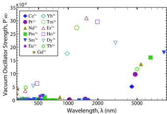
Figure 1: (Color online) Plot of the magnetic dipole ground state absorption lines and corresponding MD oscillator strengths for all trivalent lanthanide ions between $300$ and $10000$ nm.

We first calculate the oscillator strengths for all ground state MD absorption lines in the trivalent lanthanide series. (The formulas used for this calculation are provided in Appendix B.) Our results found $468$ non-zero MD absorption lines, including 84 transitions between $300$ nm and $10$ $\upmu{}$m; the vacuum oscillator strengths, $P_{MD}^{\prime}{}$, of these transitions are plotted in Fig. 1. Table 2 shows a list of the most prominent ground state absorption lines, restricted to the energy bounds and minimum oscillator strengths used in Table 1 of  Carnall et al. (1968)

Table 2: Calculated MD vacuum oscillator strengths for trivalent lanthanides.

	$SLJ$	$S^{\prime}L^{\prime}J^{\prime}$	E(cm-1)		$\lambda{}(nm)$	$P_{MD}^{\prime}{}\times{}10^{8}$			$SLJ$	$S^{\prime}L^{\prime}J^{\prime}$	E(cm-1)		$\lambda{}(nm)$	$P_{MD}^{\prime}{}\times{}10^{8}$
Ce3+	${}^{2}F_{5/2}$	${}^{2}F_{7/2}$	2266		4414	5.24		Gd3+	${}^{8}S_{7/2}$	${}^{6}D_{9/2}$	39 524	39779	253	0.04	0.03
Pr3+	${}^{3}H_{4}$	${}^{3}H_{5}$	2092	2322	4781	9.86	9.76			${}^{6}D_{7/2}$	40 647	40712	246	0.55	0.39
		${}^{3}F_{3}$	6290	6540	1590	0.02	0.02			${}^{6}D_{5/2}$	40 928	40977	244	0.29	0.20
		${}^{3}F_{4}$	6720	6973	1488	0.50	0.49	Tb3+	${}^{7}F_{6}$	${}^{7}F_{5}$	1999	2112	5003	11.90	12.11
		${}^{1}G_{4}$	9734	9885	1027	0.27	0.25			${}^{5}G_{6}$	27 004	26425	370	5.01	5.03
Nd3+	${}^{4}I_{9/2}$	${}^{4}I_{11/2}$	1829	2007	5468	13.75	14.11			${}^{5}G_{5}$	28 252	27795	354	0.38	0.36
		${}^{2}H_{9/2}$	12 167	12738	822	1.25	1.12			${}^{5}L_{6}$	30 042	29550	333	0.14	0.14
		${}^{4}F_{9/2}$	14 540	14854	688	0.18	0.20			${}^{5}H_{7}$	31 843	31537	314	0.05	0.06
		${}^{2}G_{7/2}$	16 892	17333	592	0.02	0.02			${}^{5}H_{6}$	33 279	33027	300	0.37	0.46
		${}^{2}G_{9/2}$	19 266		519	0.02				${}^{5}H_{5}$	34 182	33879	293	0.08	0.03
		${}^{2}I_{11/2}$	29 454	28624	340	0.45	0.05			${}^{5}F_{5}$	35 441	34927	282	2.11	1.87
		${}^{2}H_{11/2}$	34 646		289	0.05				${}^{5}G_{6}$	41 329	41082	242	0.26	0.23
Pm3+	${}^{5}I_{4}$	${}^{5}I_{5}$	1462	1577	6841	16.23	16.36			$(^{5}G$,${}^{5}K)_{5}$	41 605		240	0.02
		${}^{5}F_{4}$	14 432	14562	693	0.07	0.08			${}^{5}K_{6}$	44 324		226	0.04
		$(^{3}H$,${}^{5}G)_{4}$	17 376	17327	575	1.23	1.30	Dy3+	${}^{6}H_{15/2}$	${}^{6}H_{13/2}$	3316	3506	3016	21.73	22.68
		${}^{5}G_{3}$	17 896		559	0.02				${}^{4}I_{15/2}$	22 691	22293	441	5.48	5.95
		${}^{5}G_{4}$	20 038	20181	499	0.46	0.26			${}^{4}K_{17/2}$	25 967	26365	385	0.10	0.09
		${}^{3}G_{4}$	24 499	23897	408	0.09	0.11			${}^{4}I_{13/2}$	26 050	25919	384	0.51	0.41
		${}^{3}G_{5}$	27 022		370	0.02				${}^{4}M_{15/2}$	29 534	29244	339	0.61	0.69
		${}^{3}I_{5}$	28 207	27916	355	0.49	0.23			${}^{4}M_{17/2}$	29 740	30892	336	0.02	0.03
		${}^{3}H_{4}$	36 389	35473	275	0.04	0.04			$(^{4}K$,${}^{4}M)_{15/2}$	30 846	31795	324	0.23	0.12
Sm3+	${}^{6}H_{5/2}$	${}^{6}H_{7/2}$	1069	1080	9355	18.12	17.51			$(^{4}K$,${}^{4}L)_{13/2}$	33 321	33776	300	0.20	0.37
		${}^{6}F_{3/2}$	6416	6641	1559	0.03	0.02			${}^{4}H_{13/2}$	33 924	33471	295	1.41	0.60
		${}^{6}F_{5/2}$	6883	7131	1453	0.11	0.08			${}^{4}L_{15/2}$	36 261		276	0.02
		${}^{4}G_{5/2}$	18 116	17924	552	1.73	1.76			$(^{4}L$,${}^{4}K)_{13/2}$	36 666		273	0.02
		${}^{4}F_{3/2}$	18 918	18832	529	0.03	0.03			$(^{2}K$,${}^{2}L)_{15/2}$	38 434	38811	260	0.15	0.09
		${}^{4}G_{7/2}$	20 172	20014	496	0.10	0.05	Ho3+	${}^{5}I_{8}$	${}^{5}I_{7}$	5064	5116	1975	29.72	29.47
		${}^{4}F_{5/2}$	22 177	22098	451	0.45	0.45			${}^{3}K_{8}$	20 715	21308	483	6.46	6.39
		${}^{4}F_{7/2}$	24 889		402	0.02				${}^{3}K_{7}$	25 636	26117	390	0.28	0.28
		${}^{4}H_{7/2}$	28 715	28396	348	0.04	0.67			${}^{3}L_{9}$	28 873	29020	346	0.14	0.12
		${}^{4}G_{5/2}$	30 079	30232	332	0.04	0.03			${}^{3}L_{8}$	33 577	34206	298	0.21	0.17
		${}^{4}H_{7/2}$	42 572		235	0.19				${}^{3}I_{7}$	37 258	38470	268	0.24	0.36
		${}^{4}G_{5/2}$	43 021	42714	232	0.19	0.02	Er3+	${}^{4}I_{15/2}$	${}^{4}I_{13/2}$	6534	6610	1528	31.14	30.82
Eu3+	${}^{7}F_{0}$	${}^{7}F_{1}$	399	350	25044	18.68	17.73			${}^{2}K_{15/2}$	27 315	27801	366	3.66	3.69
		${}^{5}D_{1}$	19 264	19026	519	1.69	1.62			${}^{2}K_{13/2}$	32 597	33085	307	0.05	0.11
		${}^{5}F_{1}$	33 755	33429	296	1.24	2.16			${}^{2}L_{17/2}$	41 022	41686	244	0.03	0.03
		${}^{3}P_{1}$	38 891		257	0.05		Tm3+	${}^{3}H_{6}$	${}^{3}H_{5}$	8205	8390	1219	27.41	27.25
		${}^{5}D_{1}$	41 557		241	0.29				${}^{2}I_{6}$	34 212	34886	292	1.42	1.40
Gd3+	${}^{8}S_{7/2}$	${}^{6}P_{7/2}$	32 557	32224	307	4.28	4.13	Yb3+	${}^{2}F_{7/2}$	${}^{2}F_{5/2}$	10 248	10400	976	17.76	17.76
		${}^{6}P_{5/2}$	33 169	32766	301	2.42	2.33

By comparison, we find 13 additional MD transitions that are not listed in Ref. Carnall et al., 1968. While most of these new absorption lines are relatively weak, $P_{MD}^{\prime}{}\leq{}5\times 10^{-10}$, several exhibit significant MD oscillator strengths, including the ${}^{2}F_{5/2}\rightarrow{}^{2}F_{7/2}$ ($4.14$ $\upmu$m) transition in Ce³⁺, ${}^{6}H_{5/2}\rightarrow{}^{4}H_{7/2}$ ($235$ nm) transition in Sm³⁺, and the ${}^{7}F_{0}\rightarrow{}^{5}D_{1}$ ($241$ nm) transition in Eu³⁺ that have vacuum oscillator strengths of $5.24\times 10^{-8}$, $1.9\times 10^{-9}$ and $2.9\times 10^{-9}$ respectively. As well as finding additional absorption lines, these calculations provide a more accurate prediction of transition wavelengths. For example, the ${}^{4}I_{15/2}\rightarrow{}^{4}I_{13/2}$ transition in Er³⁺ is here calculated to occur at $1528$ nm, closer to the observed $1543$ nm center wavelengthWeber (1967) than the $1513$ nm value reported in Ref. Carnall et al., 1968. However, it is worth noting that the oscillator strengths are not significantly changed by the inclusion of higher order terms in the free ion Hamiltonian, as evidenced by the side-by-side comparison of $P_{MD}^{\prime}{}$ values in Table 2. As further validation, our values also compare favorably with the Hartree-Fock code developed by R.D. Cowan and maintained at Los Alamos National Laboratory, which predicts that the ${}^{4}I_{15/2}\rightarrow{}^{4}I_{13/2}$ transition in the $4f^{11}$ configuration of Er³⁺ should occur at 1495.5 nm with an oscillator strength of 31.75$\times$10^-8, which is within 2% of our calculated value of 31.14$\times$10^-8. For reference, a tabulated version of the all non-zero MD ground state absorption lines between $300$ and $10$ $\mu{}$m is provided in Table S1 of the Supplemental Material.

III.2 Magnetic Dipole Emission Lines

Beyond ground state absorption lines, there are MD transitions that occur solely between two excited states. Some of these excited transitions, such as the ${}^{5}D_{0}\rightarrow{}^{7}F_{1}$ transition in Eu³⁺ and ${}^{5}D_{4}\rightarrow{}^{7}F_{5}$ transition in Tb³⁺ have been identified experimentally.Freed and Weissman (1941); Taminiau et al. (2012) However, there have been no exhaustive studies of MD emission in all trivalent lanthanide ions. Here, we use calculations to perform such a search. We proceed to tabulate all non-zero MD emission lines between $300$ and $1700$ nm. A total of 1927 non-zero MD emission lines were found throughout the lanthanide series. In Tables S2-S13 of the Supplemental Material we provide a complete list of all such transitions, grouping them by originating excited level to allow for a more convenient comparison in future experimental studies. A more condensed table of strong transitions with vacuum emission rates, $A^{\prime}_{MD}$, greater than 5 $s^{-1}$ is shown in Table 3.

Table 3: Calculated MD vacuum spontaneous emission rates.

	$SLJ$	$S^{\prime}L^{\prime}J^{\prime}$	$\lambda$ (nm)	$A_{MD}^{\prime}{}$ $(s^{-1})$		$SLJ$	$S^{\prime}L^{\prime}J^{\prime}$	$\lambda$ (nm)	$A_{MD}^{\prime}{}$ $(s^{-1})$
Sm3+	${}^{4}G_{11/2}$	${}^{6}F_{11/2}$	477	7.14	Dy3+	$(^{4}F,$${}^{4}D)_{5/2}$	${}^{6}F_{7/2}$	533	5.13
	${}^{4}D_{3/2}$	${}^{6}F_{5/2}$	487	5.44		${}^{6}P_{3/2}$	${}^{6}F_{5/2}$	555	8.89
	${}^{4}D_{1/2}$	${}^{6}F_{3/2}$	504	5.93		$(^{2}K,$${}^{2}L)_{15/2}$	${}^{4}I_{15/2}$	635	9.75
Eu3+	${}^{5}F_{2}$	${}^{7}F_{1}$	304	5.49		$(^{4}P,$${}^{6}P)_{3/2}$	${}^{6}F_{5/2}$	676	5.94
	${}^{5}F_{4}$	${}^{7}F_{5}$	336	5.62		${}^{4}F_{9/2}$	${}^{6}F_{11/2}$	734	11.72
	${}^{5}F_{5}$	${}^{7}F_{6}$	339	5.44		${}^{4}G_{9/2}$	${}^{4}G_{11/2}$	896	6.64
	${}^{5}D_{4}$	${}^{7}F_{5}$	417	5.47		$(^{2}K$,${}^{2}L)_{15/2}$	${}^{4}M_{15/2}$	1124	8.33
	${}^{5}G_{4}$	${}^{7}F_{4}$	418	6.31		$(^{4}P$,${}^{4}D)_{3/2}$	${}^{6}P_{3/2}$	1170	5.19
	${}^{5}G_{5}$	${}^{7}F_{5}$	436	8.30		${}^{4}G_{9/2}$	${}^{4}G_{11/2}$	1550	6.21
	${}^{5}G_{6}$	${}^{7}F_{6}$	455	10.51	Ho3+	$(^{3}H$,${}^{3}G)_{5}$	${}^{5}I_{6}$	361	12.20
	${}^{5}D_{3}$	${}^{7}F_{4}$	460	9.02		$(^{1}G$,${}^{3}H)_{4}$	${}^{5}I_{5}$	411	9.86
	${}^{5}D_{2}$	${}^{7}F_{3}$	505	11.58		${}^{3}F_{4}$	${}^{5}F_{5}$	422	6.73
	${}^{5}D_{1}$	${}^{7}F_{2}$	550	12.29		${}^{3}H_{6}$	${}^{5}I_{7}$	449	24.71
	${}^{3}P_{1}$	${}^{5}D_{2}$	583	16.01		$(^{1}G$,${}^{3}H)_{4}$	${}^{5}I_{4}$	449	5.05
	${}^{5}D_{0}$	${}^{7}F_{1}$	584	14.37		${}^{3}K_{8}$	${}^{5}I_{8}$	483	18.48
	${}^{3}P_{0}$	${}^{5}D_{1}$	700	24.63		${}^{3}F_{4}$	${}^{5}F_{4}$	486	5.71
	$(^{3}I$,${}^{3}H)_{6}$	${}^{5}G_{6}$	776	5.51		${}^{3}K_{7}$	${}^{5}I_{7}$	486	8.68
Gd3+	${}^{6}P_{5/2}$	${}^{8}S_{7/2}$	301	23.64		${}^{3}P_{2}$	${}^{5}S_{2}$	511	6.61
	${}^{6}P_{7/2}$	${}^{8}S_{7/2}$	307	30.24		${}^{3}F_{4}$	${}^{5}F_{3}$	538	6.47
Tb3+	${}^{5}F_{3}$	${}^{7}F_{3}$	306	6.65		$(^{5}G$,${}^{3}H)_{5}$	${}^{5}I_{6}$	543	8.35
	${}^{5}F_{2}$	${}^{7}F_{2}$	308	10.07		$(^{3}F$,${}^{3}G)_{4}$	${}^{5}I_{4}$	618	7.72
	${}^{5}F_{1}$	${}^{7}F_{1}$	310	14.40		${}^{3}F_{4}$	$(^{5}G$,${}^{3}G)_{5}$	653	16.60
	${}^{5}F_{1}$	${}^{7}F_{0}$	312	8.81		${}^{3}P_{1}$	${}^{5}S_{2}$	661	6.19
	${}^{5}G_{6}$	${}^{7}F_{6}$	370	24.35		${}^{3}D_{3}$	${}^{5}F_{4}$	672	12.32
	${}^{5}D_{0}$	${}^{7}F_{1}$	378	29.24		${}^{3}L_{8}$	${}^{3}K_{8}$	777	11.42
	${}^{5}G_{5}$	${}^{7}F_{5}$	381	14.54		${}^{3}P_{1}$	${}^{5}F_{2}$	800	5.00
	${}^{5}D_{1}$	${}^{7}F_{2}$	381	20.20		${}^{3}L_{7}$	${}^{3}K_{7}$	811	5.60
	${}^{5}D_{1}$	${}^{7}F_{0}$	392	8.21		$(^{3}H$,${}^{3}G)_{5}$	$(^{5}G$,${}^{3}H)_{5}$	1078	6.22
	${}^{5}G_{4}$	${}^{7}F_{4}$	393	9.68		$(^{3}H$,${}^{3}G)_{5}$	${}^{3}H_{6}$	1126	12.12
	${}^{5}G_{3}$	${}^{7}F_{3}$	399	5.57		$(^{5}F$,${}^{5}G)_{2}$	${}^{5}F_{3}$	1270	6.40
	${}^{5}D_{2}$	${}^{7}F_{3}$	409	17.88		$(^{5}D$,${}^{5}G)_{4}$	$(^{5}G$,${}^{3}H)_{5}$	$1438$	$6.48$
	${}^{5}D_{3}$	${}^{7}F_{4}$	427	15.49	Er3+	${}^{2}K{}_{15/2}$	${}^{4}I{}_{15/2}$	$366$	$18.20$
	${}^{5}D_{2}$	${}^{7}F_{1}$	430	7.11		${}^{2}K{}_{13/2}$	${}^{4}I{}_{13/2}$	$384$	$5.25$
	${}^{5}D_{4}$	${}^{7}F_{5}$	530	14.32		$(^{2}H$,${}^{2}G)_{9/2}$	${}^{4}I{}_{11/2}$	$392$	$5.34$
	$(^{5}D$,${}^{3}P)_{2}$	${}^{5}D_{3}$	766	17.49		${}^{4}G{}_{11/2}$	${}^{4}I{}_{13/2}$	$529$	$12.36$
Dy3+	$(^{4}G$,${}^{4}P)_{5/2}$	${}^{6}H_{7/2}$	334	5.71		${}^{2}D{}_{5/2}$	${}^{4}F{}_{7/2}$	$583$	$5.05$
	${}^{4}G_{7/2}$	${}^{6}H_{9/2}$	347	8.28		${}^{2}P{}_{1/2}$	${}^{4}S{}_{3/2}$	$668$	$11.31$
	$(^{4}G$,${}^{4}P)_{5/2}$	${}^{6}H_{5/2}$	348	5.58		${}^{2}D{}_{5/2}$	${}^{4}F{}_{7/2}$	$686$	$20.05$
	${}^{4}H_{7/2}$	${}^{6}H_{5/2}$	360	12.78		$(^{2}G$,${}^{4}F)_{9/2}$	${}^{4}I{}_{11/2}$	$733$	$8.48$
	${}^{4}G_{11/2}$	${}^{6}F_{11/2}$	361	15.99		$(^{2}P$,${}^{2}D)_{3/2}$	${}^{4}S_{3/2}$	764	5.55
	$(^{4}H$,${}^{4}G)_{9/2}$	${}^{6}F{}_{9/2}$	$362$	$6.15$		$(^{2}H$,${}^{4}G)_{11/2}$	${}^{4}I_{13/2}$	832	14.86
	${}^{4}G{}_{7/2}$	${}^{6}H{}_{7/2}$	$366$	$6.84$		$(^{2}H$,${}^{2}G)_{9/2}$	$(^{2}G$,${}^{4}F)_{9/2}$	843	11.21
	$(^{4}H$,${}^{4}G)_{11/2}$	${}^{6}F{}_{11/2}$	$375$	$5.74$		$(^{2}H$,${}^{2}G)_{9/2}$	${}^{4}G_{11/2}$	978	11.87
	$(^{4}P{}$,${}^{4}D{})_{3/2}$	${}^{6}F{}_{5/2}$	$376$	$6.62$		$(^{2}P$,${}^{2}D)_{3/2}$	${}^{4}F_{5/2}$	1081	8.19
	${}^{4}G{}_{9/2}$	${}^{6}F{}_{9/2}$	$386$	$8.45$		$(^{2}G$,${}^{4}F)_{9/2}$	${}^{4}F_{9/2}$	1101	10.35
	${}^{4}D{}_{7/2}$	${}^{6}F{}_{9/2}$	$400$	$9.44$		$(^{2}P$,${}^{2}D)_{3/2}$	${}^{4}F_{3/2}$	1111	8.56
	${}^{4}G{}_{9/2}$	${}^{6}H{}_{11/2}$	$410$	$11.35$		${}^{4}G_{9/2}$	$(^{2}H$,${}^{4}G)_{11/2}$	1276	12.21
	${}^{4}P{}_{1/2}$	${}^{6}F{}_{3/2}$	$412$	$9.28$		${}^{4}I_{13/2}$	${}^{4}I_{15/2}$	1528	10.17
	$(^{4}G{}$,${}^{4}F{})_{7/2}$	${}^{6}H{}_{9/2}$	$415$	$8.77$		${}^{4}G_{7/2}$	${}^{4}G_{9/2}$	1533	6.43
	${}^{4}P_{1/2}$	${}^{6}F_{1/2}$	421	6.67	Tm3+	$(^{3}P$,${}^{1}D)_{2}$	${}^{3}F_{3}$	430	22.93
	$(^{4}F$,${}^{4}G)_{5/2}$	${}^{6}F_{7/2}$	428	6.72		$(^{3}P$,${}^{1}D)_{2}$	${}^{3}F_{3}$	765	13.97
	${}^{4}I_{11/2}$	${}^{6}H_{11/2}$	436	5.71		${}^{1}G_{4}$	${}^{3}H_{5}$	784	22.64
	${}^{4}I_{13/2}$	${}^{6}H_{13/2}$	440	9.99		$(^{3}P$,${}^{1}D)_{2}$	${}^{3}F_{2}$	808	9.29
	${}^{4}I_{15/2}$	${}^{6}H_{15/2}$	441	18.83		$(^{3}P$,${}^{1}D)_{2}$	$(^{3}P$,${}^{1}D)_{2}$	983	12.96
	$(^{4}D$,${}^{4}G)_{5/2}$	${}^{6}H_{5/2}$	458	5.09		${}^{3}F_{3}$	${}^{3}F_{4}$	1155	10.88
	$(^{4}D$,${}^{4}G)_{5/2}$	${}^{6}F_{7/2}$	471	8.11		${}^{1}G_{4}$	${}^{3}H_{4}$	1167	5.60
	${}^{4}G_{11/2}$	${}^{6}H_{13/2}$	493	19.49		${}^{3}H_{5}$	${}^{3}H_{6}$	1219	14.55
	${}^{4}F_{3/2}$	${}^{6}F_{1/2}$	495	7.27	Yb3+	${}^{2}F_{5/2}$	${}^{2}F_{7/2}$	976	16.59
	$(^{4}D$,${}^{4}P)_{1/2}$	${}^{6}F_{3/2}$	530	10.38

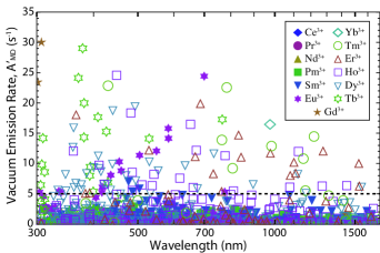
Figure 2: (Color online) Magnetic dipole emission lines and corresponding vacuum emission rates for all trivalent lanthanide ions between $300$ and $1700$ nm. Strong emission lines with vacuum rates greater than 5 $s^{-1}$ located above the dashed line are listed in Table III.

As shown in Figure 2, there are many strong MD transitions thoughout the ultraviolet, visible, and near infrared spectra. In addition to transitions which have been previously identified through ground state calculations or experimental characterization, there are many more MD emission lines which could be of practical interest.

In the ultraviolet spectrum, MD transitions in Er³⁺, Gd³⁺, and Tb³⁺ are particularly strong. The ${}^{6}P_{5/2}\rightarrow{}^{8}S_{7/2}$ ($301$ nm) and ${}^{6}P_{7/2}\rightarrow{}^{8}S_{7/2}$ ($307$ nm) transitions in Gd³⁺ have vacuum emission rates of 23.64 and 30.24 $s^{-1}$, respectively. Similarly, the ${}^{2}K_{15/2}\rightarrow{}^{4}I_{15/2}$ ($366$ nm) transition in Er³⁺ has a vacuum emission rate of 18.20 $s^{-1}$. Note that these transitions to the ${}^{4}I_{15/2}$ ground state in Er³⁺ and the ${}^{8}S_{7/2}$ ground state in Gd³⁺ could have been inferred from the absorption lines discussed in the previous section. However, the strong UV transitions in Tb³⁺ occur between excited states, such as the ${}^{5}D_{0}\rightarrow{}^{7}F_{1}$ ($378$ nm) and ${}^{5}D_{1}\rightarrow{}^{7}F_{2}$ ($381$ nm) which have vacuum emission rates of 29.24 and 20.20 $s^{-1}$, respectively. These ${}^{5}D_{J}\rightarrow{}^{7}F_{J+1}$ Tb³⁺ transitions are the higher level analogues to the experimentally characterized ${}^{5}D_{4}\rightarrow{}^{7}F_{5}$ ($530$ nm) excited state transition.

Throughout the visible spectrum, there are strong MD transitions in Eu³⁺, Ho³⁺, and Tb³⁺. Similar to the UV transitions in Tb³⁺, many of the visible MD transitions in Eu³⁺ and Tb³⁺ are higher level analogues to the previously known ${}^{5}D_{J}\rightarrow{}^{7}F_{J+1}$ transitions. In Eu³⁺, the well-known ${}^{5}D_{0}\rightarrow{}^{7}F_{1}$ ($584$ nm) transition has a calculated vacuum emission rate of 14.37 $s^{-1}$. In addition to this yellow emission line, there are also higher energy blue and green MD transitions in Eu³⁺, including the ${}^{5}D_{1}\rightarrow{}^{7}F_{2}$ ($550$ nm), ${}^{5}D_{2}\rightarrow{}^{7}F_{3}$ ($505$ nm), and ${}^{5}D_{3}\rightarrow{}^{7}F_{4}$ ($460$ nm) that have vacuum emission rates near 10 $s^{-1}$ each. Likewise, in addition to the green ${}^{5}D_{4}\rightarrow{}^{7}F_{5}$ ($530$ nm) line and higher ultraviolet transitions, Tb³⁺ also has several blue-violet MD transitions, such as ${}^{5}D_{2}\rightarrow{}^{7}F_{3}$ ($409$ nm) and ${}^{5}D_{3}\rightarrow{}^{7}F_{4}$ ($420$ nm) which have vacuum emission rates greater than 15 $s^{-1}$. Trivalent Holmium (Ho³⁺) also exhibits several strong blue MD transitions. Two prominent Ho³⁺ transitions are the ${}^{3}K_{8}\rightarrow{}^{5}I_{8}$ ($483$ nm) ground state transition and the ${}^{3}H_{6}\rightarrow{}^{5}I_{7}$ ($449$ nm) excited state transition, which have vacuum emission rates of 18.48 and 24.71 $s^{-1}$, respectively.

Most interestingly from an experimental perspective, there are also many strong MD transitions in the near-infrared spectrum. At these longer wavelengths, the design and fabrication of metamaterials,Zhang et al. (2005); Enkrich et al. (2005); Valentine et al. (2008); Sersic et al. (2009); Ameling and Giessen (2010); Xiao et al. (2010); Soukoulis and Wegener (2011) resonant optical antennas,Novotny (2007); Curto et al. (2010); Dregely et al. (2011); Barnard et al. (2011) photonic crystals,Burresi et al. (2010); Vignolini et al. (2010) and plasmonic waveguidesCharbonneau et al. (2000); Weeber et al. (2003, 2005); Ditlbacher et al. (2005); Bozhevolnyi et al. (2006); Zia et al. (2006); Buckley and Berini (2007) are more established. Although some transitions in this regime originate from excited states that would require deep UV excitation, there are a number of transitions in Dy³⁺, Er³⁺, Tm³⁺, and Yb³⁺ that can be pumped at visible or near-IR wavelengths and are thus strong candidates for experimental use. These include several ground state transitions that could be identified from the absorption line calculations in the previous section, including the ${}^{4}I_{15/2}\rightarrow{}^{4}I_{13/2}$ ($1528$ nm) transition in Er³⁺, the ${}^{3}H_{5}\rightarrow{}^{3}H_{6}$ ($1219$ nm) transition in Tm³⁺, and the ${}^{2}F_{5/2}\rightarrow{}^{2}F_{7/2}$ ($976$ nm) transition in Yb³⁺. Here, we calculate the MD vacuum emission rates of these transitions to be 10.17, 14.55, and 16.59 $s^{-1}$, respectively. Our calculations also reveal several promising excited state MD transitions. These include the ${}^{4}F_{9/2}\rightarrow{}^{6}F_{11/2}$ ($734$ nm) transition in Dy³⁺, the ${}^{1}G_{4}\rightarrow{}^{3}H_{5}$ ($784$ nm) transition in Tm³⁺, and the $(^{2}H,^{4}G)_{11/2}\rightarrow{}^{4}I_{13/2}$ ($832$ nm) transition in Er³⁺ that have vacuum emission rates of 11.72, 22.64, and 14.86 $s^{-1}$, respectively.

Table 4: Calculated MD Branching Ratios for Yb³⁺ Transition in Different Host Materials

Host	Measured Lifetime	Refractive Index	MD Emission Rate	MD Branching Ratio
	$\tau$ (ms)	$n_{r}$	$A_{MD}$ (s-1)	$\beta_{MD}$
LiYF4	2.16	1.455	51.10	11.0%
LaF3	2.22	1.597	67.57	15.0%
SrF2	9.72	1.438	49.33	48.0%
BaF2	8.2	1.473	53.02	43.5%
KCaF3	2.7	1.378	43.41	11.7%
KY3F${}_{1}0$	2.08	1.5	55.99	11.6%
Rb2NaYF6	10.84	1.403	45.82	49.7%
BaY2F8	2.04	1.521	58.38	11.9%
Y2SiO5	1.04	1.79	95.15	9.9%
Y3Al5O12	1.08	1.82	100.0	10.8%
YAIO3	0.72	1.956	124.2	8.9%
Ca5(PO4)3F	1.08	1.63	71.85	7.8%
LuPO4	0.83	1.83 (est.)	101.7	8.4%
LiYO2	1.13	1.82 (est.)	100.0	11.3%
ScBO3	4.8	1.84	103.3	49.6%

Of the seven strong near-infrared lines identified above, the four transitions between 700 and 1000 nm are the most promising candidates for immediate experimental study. Unlike longer wavelength transitions such as the 1.5 $\upmu$m transition in Er³⁺, these MD transitions occur in a spectral region where they are still readily observed by silicon photodetectors. (For example, back-illuminated CCD cameras such as the Pixis 1024B from Princeton Instruments exhibit greater than 50% quantum efficiency up to 900nm.) Nevertheless, these transitions also occur at sufficiently long wavelengths that resonant plasmonic and nanophotonic structures can be readily fabricated.

For experimental studies, it will also be important to select appropriate host materials to maximize MD emission. In particular, to enhance the MD contribution to mixed transitions, it will be helpful for lanthanide ions to be substitutionally doped into centrosymmetric sites where ED transitions are strictly forbidden. Table 4 shows the calculated MD branching ratios for the Yb³⁺ ${}^{2}F_{5/2}\rightarrow{}^{2}F_{7/2}$ ($976$ nm) transition in different host materials. These calculations were performed by comparing the total decay rate ($\Gamma_{total}=1/{\tau}$), as inferred from experimental lifetime data in the literature,DeLoach et al. (1993) with the MD spontaneous emission rates ($A_{MD}=A_{MD}^{\prime}{}$ $n_{r}^{3}$)Rikken and Kessener (1995); Zampedri et al. (2007); Duan et al. (2011) predicted from the vacuum rates in Table 3. The MD branching ratio is thus defined as: $\beta_{MD}=A_{MD}/{\Gamma_{total}}$. Note that the MD branching ratio for this Yb³⁺ transition varies significantly in different host materials. In centrosymmetric hosts such as SrF₂, Rb₂NaYF₆, and ScBO₃, it is possible to have $\sim$50% of all decay processes result in MD emission. In more common materials, such as yttrium aluminum garnet (YAG, Y₃Al₅O₁₂), MD emission still accounts for $\sim$10% of all decay processes.

The relatively simple two-level energy structure of Yb³⁺ means that MD emission can naturally account for a significant contribution to the overall decay. Other, more complex energy level structures, such as in Dy³⁺ and Tm³⁺, mean that there are more decay paths from any particular excited state. These transitions are thus interesting candidates for enhancing MD emission. For instance, the lifetime of the ${}^{4}F_{9/2}$ excited level in Dy³⁺ ranges from 300 $\upmu$s in LiNbO₃ Dominiak-Dzik et al. (2004) to 2.36 ms in Y₃Sc₂Ga₃O₁₂ (YSGG) Sardar et al. (2004) leading to respective branching ratios of 0.35% and 2.77% for the associated ${}^{4}F_{9/2}\rightarrow{}^{6}F_{11/2}$ MD transition. Similar branching ratios were found by analyzing the ${}^{1}G_{4}\rightarrow{}^{3}H_{5}$ transition in Tm³⁺.Guery et al. (1988); Pisarski et al. (2004); Sokólska et al. (2000)

III.3 Electric Quadrupole Calculations

In the multipolar expansion of light-matter interactions, MD terms are generally included in the same order as EQ terms, because they both scale with spatial derivatives of the electric field. Thus, a common question is to what extent EQ transitions compete with MD transitions. For completeness, we have calculated the oscillators strengths for all EQ ground state absorption lines and the spontaneous emission rates for all EQ emission lines. The EQ oscillator strengths and transition rates were found to be significantly smaller than those for MD transitions.

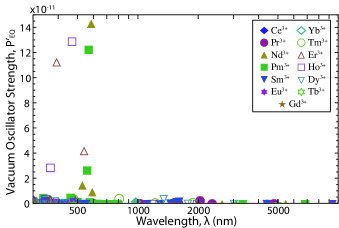
Figure 3: (Color online) Plot of all electric quadruple ground state absorption lines and corresponding EQ oscillator strengths for all trivalent lanthanide ions between $300$ and $10000$ nm.

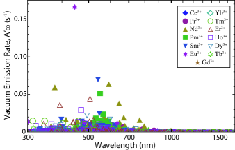
Figure 4: (Color online) Plot of all electric quadrupole emission lines and corresponding EQ vacuum emission rates for all trivalent lanthanide ions between $300$ and $1700$ nm.

The strongest EQ transition was the $(^{5}D,^{5}P)_{2}\rightarrow{}^{5}D_{0}$ transition in Eu³⁺ with a vacuum emission rate of $0.17$ $s^{-1}$. While the emission rate for EQ transitions scales with $n_{r}^{5}$, this rate is approximately 30 times weaker than the weakest MD transition presented in Table 3. Most transitions mediated by EQ interactions have an emission rate on the order of $0.01$ s^-1 and would thus require significant enhancement to even be observed. Figures 3 and 4 show the vacuum oscillator strengths and emission rates, respectively, for EQ absorption lines and EQ emission lines. A complete tabulation of all 236 EQ absorption lines (Table S14) and all 3079 EQ emission lines (Tables S15-S25) between $300$ and $1700$ nm is provided in the Supplemental Material. These calculations confirm that EQ transitions in trivalent lanthanide ions are negligible in comparison to the MD transitions calculated above.

IV Conclusion

Using a detailed free ion Hamilitonian, we have calculated all non-zero MD ground state absorption lines and corresponding oscillator strengths throughout the full trivalent lanthanide series. These values are well documented in the literature, and we observed good agreement between our results and those found in Ref. Carnall et al., 1968. Using this detailed Hamiltonian, we then calculated all non-zero MD and EQ emission lines and their respective emission rates for all trivalent lanthanide ions. Although the EQ emission rates were found to be negligible, our calculations revealed vastly more MD emission lines than previously identified by ground state calculations or experimental investigation.

In the specific spectral range from 300 – 1700 nm, we identified 1927 MD transitions, including 117 lines with vacuum spontaneous emission rates $A^{\prime}{}_{MD}>$ 5 s^-1. Of these transitions, four were identified as the most promising for experimental exploration: ${}^{4}F_{9/2}\rightarrow{}^{6}F_{11/2}$ ($734$ nm) in Dy³⁺, ${}^{1}G_{4}\rightarrow{}^{3}H_{5}$ ($784$ nm) in Tm³⁺, $(^{2}H,^{4}G)_{11/2}\rightarrow{}^{4}I_{13/2}$ ($832$ nm) in Er³⁺, and ${}^{2}F_{5/2}\rightarrow{}^{2}F_{7/2}$ ($976$ nm) in Yb³⁺. These near-IR transitions occur at wavelengths for which resonant devices are easily fabricated, yet still emit within the detection range of silicon photodetectors.

We subsequently demonstrated how free ion calculations can be used to analyze and predict MD emission within a range of host materials. We compared the calculated emission rates with experimental lifetime data from the literature to approximate MD branching ratios, and for the specific case of the ${}^{2}F_{5/2}$ excited level in Yb³⁺, showed how MD emission can account for up to $\sim$50% of all decay processes. These calculations highlighted the importance of selecting appropriate hosts, especially those with high centrosymmetry and refractive indices, to maximize MD contributions.

These results and the associated tables in the Supplemental Material can thus be used to guide the study of magnetic light-matter interactions in trivalent lanthanide ions. Beyond the well-known MD emission lines in Eu³⁺ and Er³⁺, there are many permutations of ions and hosts in which MD emission can likely be observed. While further study is needed to find the most practical combinations, these comprehensive calculations provide a solid foundation from which to begin this search, and they provide a firm set of numbers with which to analyze future experimental data. The tabulated values may also be helpful in studying the potential role of MD transitions in more complex processes such as upconversion Chan et al. (2012) and quantum cutting Wegh et al. (1999). These same calculations can also help focus the design of optical structures to enhance MD emission. For example, emission wavelengths, transition rates, and branching ratios can be used as the starting point for simulating the effects of optical antennas and metamaterials on MD transitions. Combining these quantum-mechanical calculations with experimental measurements and electromagnetic simulations can expand the toolkit with which to access the naturally occurring MD transitions of lanthanide ions.

Appendix A Free Ion Hamiltonian

Closed form expressions of the interaction terms used in these calculations are provided below. These expressions are well defined through many different publications and are provided here for reference purposes.

A.1 Coefficients of Fractional Parentage

When describing a particular term in the $l^{\text{n}}$ configuration, one must realize that there could be multiple ways in which to arrive at that term from the $l^{\text{n-1}}$ configuration. There is an approach to this problem that was developed by Giulio Racah,Racah (1942a, b, 1943, 1949) which defines the terms of the $l^{\text{n}}$ configuration in terms of $l^{\text{n-1}}$. The terms of $l^{\text{n-1}}$ are known as the parents of the corresponding daughters $l^{\text{n}}$. These coefficients of fractional parentage (CFP) need only be calculated once. For this paper, the CFP were not calculated directly but an electronic version of the tables produced by Nielson and Koster (1963) was used instead. All subsequent calculations were made using these values. The CFP are denoted by $\left(\psi\{|\psi\right)$. Due to the fact that a particular state might appear in more than one configuration, such as in both the $4f^{\text{n}}$ and $4f^{\text{n+2}}$ configurations, a method to distinguish when a state appears is necessary. This is accomplished by using the seniority number, which can take integer values from $1$ to $7$, indicating in which $4f^{\text{n}}$ configuration a state first appears.

A.2 Electrostatic Interaction

The electrostatic interaction occurs between configurations with two or more electrons. This is a result of the Coulomb repulsion between the two electrons. It is calculated from two single electron wavefunctions. The electrostatic interaction is diagonal in both J and S values and the matrix elements are found using the following expression:Cowan (1981)

$$\left<l^{n}\psi^{\prime}L^{\prime}S\left|f_{k}\right|l^{n}\psi{}LS\right>=\frac{1}{2}\left<l\left|C^{(k)}\right|l\right>^{2}\biglb(\frac{1}{2L+1}$$

$$\times{}\sum_{\bar{\psi},\bar{L}}\left<l^{n}\bar{\psi}\bar{L}S\left|U^{(k)}\right|l^{n}\psi^{\prime}L^{\prime}S\right>\left<l^{n}\bar{\psi}\bar{L}S\left|U^{(k)}\right|l^{n}\psi LS\right>$$

$$-\delta_{\psi\bar{\psi}}\frac{n(4l+2-n)}{(2l+1)(4l+1)}\bigrb).$$

$C^{(k)}$ is the irreducible tensor defined by Racah,Racah (1942b) and $U^{(k)}$ is the irreducible tensor tabulated by Nielson and Koster.Nielson and Koster (1963) Since we are concerned with $f^{\text{n}}$ configurations, we used $l=3$ for all calculations. Again, we are using the notation in which $\psi{}$ represents all other quantum numbers that are not specifically mentioned.

A.3 Spin-Orbit Interaction

The spin-orbit interaction is, in essence, a dipole-dipole interaction. The spin-orbit interaction is diagonal in $J$ but not in $L$ or $S$. We calculated this interaction using the following formula:

$$\left<f^{n}\psi^{\prime}L^{\prime}S^{\prime}\left|A_{SO}\right|f^{n}\psi{}LS\right>=(-1)^{J+L+S^{\prime}}\left\{\begin{array}[]{c c c}L&L^{\prime}&1\\ S^{\prime}&S&J\\ \end{array}\right\}$$

$$\times\left<f^{n}\psi^{\prime}L^{\prime}S^{\prime}\left|V^{(11)}\right|f^{n}\psi LS\right>.$$

Here we are using the conventional notation for the Racah 6-j symbols and $V^{(11)}$ is the irreducible tensor tabulated by Nielson and Koster (1963).

A.4 Two-Body Interaction

For configurations with two or more valence electrons (or holes), $4f^{2}$ to $4f^{12}$, two-body interactions are used to help correct for the use of single electron wavefunctions. The first term in this correction was discovered by Trees (1952). The other two terms are calculated using the Racah numbers and the Casimir operator $G$.Trees and Jørgensen (1961) The eigenvalues of the Casimir operator on the groups $R_{7}$ and $G_{2}$ can be found in Wybourne (1965).

A.5 Three-Body Interaction

The three-body interaction terms are analogous to the two-body but exist for only $4f^{3}$ to $4f^{11}$. The form of this operator is:Hansen et al. (1996)

$$\left<f^{\text{n}}\psi\left|t_{i}\right|f^{\text{n}}\psi^{\prime}\right> = \frac{n}{n-3}$$

$$\times \sum_{\bar{\psi},\bar{\psi^{\prime}}}(\psi\{|\bar{\psi})(\psi^{\prime}\{|\bar{\psi^{\prime}})\left(f^{\text{n-1}}\bar{\psi}\left|t_{i}\right|f^{\text{n-1}}\bar{\psi^{\prime}}\right).$$

This operator is built up recursively using the values for the $4f^{3}$ states found in Tables 1 and 2 of Ref. Judd and Suskin, 1984.

A.6 Spin-Spin Interaction

The spin-spin interaction is analogous to the spin-orbit but is the interaction between the spins of two electrons. $H_{ss}$ is calculated recursively, using the reduced matrix operator $T^{(22)}$. $T^{(22)}$ is defined for the $4f^{2}$ configuration, these defined values then permit the calculation for all $4f^{\text{n}}$, $n\geq{}2$, configurations and using the following equation:Judd et al. (1968)

$$\left<f^{\text{n}}\psi\left|T^{(22)}\right|f^{\text{n}}\psi^{\prime}\right>=\delta_{J,J^{\prime}}(-1)^{S^{\prime}+L+J}$$

$$\times\sum_{\bar{\psi},\bar{\psi^{\prime}}}\left(\psi\{|\psi\right)\left\{\begin{array}[]{c c c}S^{\prime}&L^{\prime}&J\\ L&S&1\\ \end{array}\right\}\left(f^{\text{n-1}}\bar{\psi}\left|T^{(22)}\right|f^{\text{n-1}}\bar{\psi^{\prime}}\right).$$

A.7 Spin-Other-Orbit and Electrostatically Correlated Spin-Orbit Interactions

The spin-other-orbit interaction is an interaction between the spin of one electron and the orbit of another. It is only valid for $4f^{2}$ to $4f^{12}$ configurations. The electrostatically correlated spin-orbit interaction is a configuration interaction between the spin of an electron in one configuration with the orbit of an electron residing in a different configuration. These terms were grouped together for calculation by Judd, Crosswhite and Crosswhite.Judd et al. (1968) The following form was used:Chen et al. (2007)

$$\left<f^{\text{n}}\psi\left|T^{(11)}+t^{(11)}-az_{13}\right|f^{\text{n}}\psi^{\prime}\right>=\delta_{J,J^{\prime}}(-1)^{S^{\prime}+L+J}$$

$$\times{}\sum_{\bar{\psi},\bar{\psi^{\prime}}}\left(\psi\{|\psi\right)\left\{\begin{array}[]{c c c}S^{\prime}&L^{\prime}&J\\ L&S&1\\ \end{array}\right\}$$

$$\times{}\left(f^{\text{n-1}}\bar{\psi}\left|T^{(11)}+t^{(11)}-az_{13}\right|f^{\text{n-1}}\bar{\psi^{\prime}}\right).$$

Both $T^{(11)}$ and $t^{(11)}$ are reduced matrix operators. These reduced matrix operators in addition to the values $a$ and $z_{13}$ are defined for the $4f^{2}$ configuration in Refs. Judd et al., 1968 and Chen et al., 2007.

Appendix B Magnetic Dipole Transitions

B.1 Oscillator Strength

All MD ground state absorption lines were calculated using the following equation:Shortley (1940)

$$f_{MD}=\frac{8\pi^{2}m_{e}}{3he^{2}c}\left(\frac{n_{r}}{\lambda}\right)\frac{1}{2J+1}S_{MD},$$

where $S_{MD}$ is the magnetic dipole transition line strength. This line strength is defined as:

$$S_{MD}=\frac{e\hbar}{2m_{e}c}\sum_{\psi,\psi^{\prime}}\left|\left<\psi^{\prime}{}\left|L+g_{e}S\right|\psi{}\right>\right|^{2},$$

where $g_{e}$ is the gyromagnetic ratio of the electron. A list of all non-zero absorption lines can be found in the Supplemental Material.

B.2 Transition Rates

All MD emission lines were calculated using the following equation:Shortley (1940)

$$A_{MD}=\frac{1}{2J+1}\frac{16\pi^{3}\mu_{0}}{3h}\left(\frac{n_{r}}{\lambda}\right)^{3}S_{MD},$$

and all non-zero transitions can be found in the Supplemental Material.

Appendix C Electric Quadrupole Transitions

C.1 Oscillator Strength

All EQ ground state absorption lines were calculated using the following equation:Thorne et al. (1999)

$$f_{EQ}=\frac{112}{225}\frac{\pi^{3}a_{0}^{3}}{\alpha}\left(\frac{n_{r}}{\lambda}\right)^{3}\left<r^{2}\right>\frac{S_{EQ}}{2J+1},$$

where $S_{EQ}$ is the electric quadrupole line strength and is defined as:

$$S_{EQ}=(-1)^{S+L^{\prime}+J+2}\sqrt{(2J+1)(2J^{\prime}+1)}$$

$$\times\left\{\begin{array}[]{c c c}J&J^{\prime}&2\\ L^{\prime}&L&S\\ \end{array}\right\}\left<\psi^{\prime}{}\left|U^{(k)}\right|\psi\right>.$$

Calculated values for the expectation value of the radial wavefunctions for the lanthanide series, $\left<r^{2}\right>$, were taken from Table 21.8 in Ref. Wybourne and Smentek, 2007. A list of all non-zero absorption lines can be found in the Supplemental Material.

C.2 Transition Rates

All EQ emission lines were calculated using the following equation:Thorne et al. (1999)

$$A_{EQ}=\frac{1}{2J+1}\frac{8\pi^{5}}{5h\epsilon_{0}}\left(\frac{n_{r}}{\lambda}\right)^{5}S_{EQ}.$$

There are a total of 3079 non-zero EQ transitions between $300$ and $1700$ nm, all such transitions can be found in the Supplemental Material.

References

- Thommen and Mandel (2006) Q. Thommen and P. Mandel, Opt. Lett. 31, 1803 (2006).
- Noginova et al. (2008) N. Noginova, G. Zhu, M. Mavy, and M. A. Noginov, J. Appl. Phys. 103, 07 (2008).
- Noginova et al. (2009) N. Noginova, Y. Barnakov, H. Li, and M. A. Noginov, Opt. Exp. 17, 10767 (2009).
- Yang et al. (2009) N. Yang, Y. Tang, and A. E. Cohen, Nano Today 4, 269 (2009).
- Ni et al. (2011) X. Ni, G. V. Naik, A. V. Kildishev, Y. Barnakov, A. Boltasseva, and V. M. Shalaev, Appl. Phys. B: Lasers Opt. 103, 553 (2011).
- Taminiau et al. (2012) T. H. Taminiau, S. Karaveli, N. F. van Hulst, and R. Zia, Nat. Commun. 3, 979 (2012).
- Karaveli and Zia (2010) S. Karaveli and R. Zia, Opt. Lett. 35, 3318 (2010).
- Karaveli and Zia (2011) S. Karaveli and R. Zia, Phys. Rev. Lett. 106, 193004 (2011).
- Feng et al. (2011) T. Feng, Y. Zhou, D. Liu, and J. Li, Opt. Lett. 36, 2369 (2011).
- Grosjean et al. (2011) T. Grosjean, M. Mivelle, F. I. Baida, G. W. Burr, and U. C. Fischer, Nano Lett. 11, 1009 (2011).
- Sheikholeslami et al. (2011) S. N. Sheikholeslami, A. García-Etxarri, and J. A. Dionne, Nano Lett. 11, 3927 (2011).
- Freed and Weissman (1941) S. Freed and S. Weissman, Phys. Rev. 60, 440 (1941).
- Drexhage (1974) K. H. Drexhage, Prog. Opt. 12, 163 (1974).
- Kunz and Lukosz (1980) R. E. Kunz and W. Lukosz, Phys. Rev. B 21, 4814 (1980).
- Rikken and Kessener (1995) G. L. J. A. Rikken and Y. A. R. R. Kessener, Phys. Rev. Lett. 74, 880 (1995).
- Zampedri et al. (2007) L. Zampedri, M. Mattarelli, M. Montagna, and R. R. Gonçalves, Phys. Rev. B 75, 073105 (2007).
- Duan et al. (2011) C.-K. Duan, H. Wen, and P. A. Tanner, Phys. Rev. B 83, 245123 (2011).
- Weber (1967) M. J. Weber, Phys. Rev. 157, 262 (1967).
- Weber (1968) M. J. Weber, Phys. Rev. 171, 283 (1968).
- Carnall et al. (1968) W. T. Carnall, P. R. Fields, and K. Rajnak, J. Chem. Phys. 49, 4412 (1968).
- Klimov (2002) V. V. Klimov, Opt. Commun. 211, 183 (2002).
- Klimov and Ducloy (2000) V. V. Klimov and M. Ducloy, Phys. Rev. A 62, 043818 (2000).
- Rolly et al. (2012) B. Rolly, B. Bebey, S. Bidault, B. Stout, and N. Bonod, Phys. Rev. B 85, 245432 (2012).
- Schmidt et al. (2012) M. K. Schmidt, R. Esteban, J. J. Sáenz, I. Suárez-Lacalle, S. Mackowski, and J. Aizpurua, Opt. Express 20, 13636 (2012).
- Zurita-Sánchez and Novotny (2002a) J. R. Zurita-Sánchez and L. Novotny, J. Opt. Soc. Am. B 19, 1355 (2002a).
- Zurita-Sánchez and Novotny (2002b) J. R. Zurita-Sánchez and L. Novotny, J. Opt. Soc. Am. B 19, 2722 (2002b).
- Klimov and Ketokhov (2005) V. V. Klimov and V. S. Ketokhov, Laser Phys. 15, 61 (2005).
- Klimov and Ducloy (2005) V. V. Klimov and M. Ducloy, Phys. Rev. A 72, 043809 (2005).
- Tojo et al. (2004) S. Tojo, M. Hasuo, and T. Fujimoto, Phys. Rev. Lett. 92, 053001 (2004).
- Tojo et al. (2005) S. Tojo, T. Fujimoto, and M. Hasuo, Phys. Rev. A 71, 012507 (2005).
- Tojo and Hasuo (2005) S. Tojo and M. Hasuo, Phys. Rev. A 71, 012508 (2005).
- Andersen et al. (2011) M. L. Andersen, S. Stobbe, A. S. Sørensen, and P. Lodahl, Nat. Phys. 7, 215 (2011).
- Kern and Martin (2012) A. M. Kern and O. J. F. Martin, Phys. Rev. A 85, 022501 (2012).
- Klimov et al. (2012) V. V. Klimov, D. V. Guzatov, and M. Ducloy, Europhys. Lett. 97, 47004 (2012).
- Filter et al. (2012) R. Filter, S. Mühlig, T. Eichelkraut, C. Rockstuhl, and F. Lederer, Phys. Rev. B 86, 035404 (2012).
- Werts et al. (2002) M. H. V. Werts, R. T. F. Jukes, and J. W. Verhoeven, Phys. Chem. Chem. Phys. 4, 1542 (2002).
- Snoeks et al. (1995) E. Snoeks, A. Lagendijk, and A. Polman, Phys. Rev. Lett. 74, 2459 (1995).
- Ambati et al. (2008) M. Ambati, S. H. Nam, E. Ulin-Avila, D. A. Genov, G. Bartal, and X. Zhang, Nano Lett. 8, 3998 (2008).
- Carnall et al. (1989) W. T. Carnall, G. L. Goodman, K. Rajnak, and R. S. Rana, J. Chem. Phys. 90, 3443 (1989).
- Note (1) A web interface to the Cowan code is available at http://aphysics2.lanl.gov/tempweb/lanl/. Although this interface cannot be directly used to calculate MD oscillator strengths, the mixing coefficients for the intermediate coupling states can be used in combination with the expressions in Appendix B to calculate MD transition rates and strengths.
- Note (4) See Supplemental Material for a complete tabulation of all nonzero MD and EQ transitions between 300 and 1700 nm for each trivalent lanthanide ion.
- Zhang et al. (2005) S. Zhang, W. Fan, N. C. Panoiu, K. J. Malloy, R. M. Osgood, and S. R. J. Brueck, Phys. Rev. Lett. 95, 137404 (2005).
- Enkrich et al. (2005) C. Enkrich, M. Wegener, S. Linden, S. Burger, L. Zschiedrich, F. Schmidt, J. F. Zhou, T. Koschny, and C. M. Soukoulis, Phys. Rev. Lett. 95, 203901 (2005).
- Valentine et al. (2008) J. Valentine, S. Zhang, T. Zentgraf, E. Ulin-Avila, D. A. Genov, G. Bartal, and X. Zhang, Nature 455, 376 (2008).
- Sersic et al. (2009) I. Sersic, M. Frimmer, E. Verhagen, and A. F. Koenderink, Phys. Rev. Lett. 103, 213902 (2009).
- Ameling and Giessen (2010) R. Ameling and H. Giessen, Nano Lett. 10, 4394 (2010).
- Xiao et al. (2010) S. Xiao, V. P. Drachev, A. V. Kildishev, X. Ni, U. K. Chettiar, H.-K. Yuan, and V. M. Shalaev, Nature 466, 735 (2010).
- Soukoulis and Wegener (2011) C. M. Soukoulis and M. Wegener, Nat. Photonics 5, 523 (2011).
- Novotny (2007) L. Novotny, Phys. Rev. Lett. 98, 266802 (2007).
- Curto et al. (2010) A. G. Curto, G. Volpe, T. H. Taminiau, M. P. Kreuzer, R. Quidant, and N. F. van Hulst, Science 329, 930 (2010).
- Dregely et al. (2011) D. Dregely, R. Taubert, J. Dorfmüller, R. Vogelgesang, K. Kern, and H. Giessen, Nat. Commun. 2, 267 (2011).
- Barnard et al. (2011) E. S. Barnard, R. A. Pala, and M. L. Brogersma, Nat. Nanotechnol. 6, 588 (2011).
- Burresi et al. (2010) M. Burresi, T. Kampfrath, D. van Oosten, J. C. Prangsma, B. S. Song, S. Noda, and L. Kuipers, Phys. Rev. Lett. 105, 123901 (2010).
- Vignolini et al. (2010) S. Vignolini, F. Intonti, F. Riboli, L. Balet, L. H. Li, M. Francardi, A. Gerardino, A. Fiore, D. S. Wiersma, and M. Gurioli, Phys. Rev. Lett. 105, 123902 (2010).
- Charbonneau et al. (2000) R. Charbonneau, P. Berini, E. Berolo, and E. Lisicka-Shrzek, Opt. Lett. 25, 844 (2000).
- Weeber et al. (2003) J.-C. Weeber, Y. Lacroute, and A. Dereux, Phys. Rev. B 68, 115401 (2003).
- Weeber et al. (2005) J.-C. Weeber, M. U. González, A.-L. Baudrion, and A. Dereux, Appl. Phys. Lett. 87, 221101 (2005).
- Ditlbacher et al. (2005) H. Ditlbacher, A. Hohenau, D. Wagner, U. Kreibig, M. Rogers, F. Hofer, F. R. Aussenegg, and J. R. Krenn, Phys. Rev. Lett. 95, 257403 (2005).
- Bozhevolnyi et al. (2006) S. I. Bozhevolnyi, V. S. Volkov, E. Devaux, J.-Y. Laluet, and T. W. Ebbesen, Nature 440, 508 (2006).
- Zia et al. (2006) R. Zia, J. A. Schuller, and M. L. Brongersma, Phys. Rev. B 74, 165415 (2006).
- Buckley and Berini (2007) R. Buckley and P. Berini, Opt. Exp. 15, 12174 (2007).
- DeLoach et al. (1993) L. DeLoach, S. Payne, L. Chase, L. Smith, W. Kway, and W. Krupke, IEEE J. of Quantum Electron. 29, 1179 (1993).
- Note (2) Note that crystal field effects in each host will also introduce a perturbation to the vacuum emission rates. However, for MD transitions, this effect is generally much smaller than the optical density of states correction due to the host’s refractive index. As a quantitative example, we have explicitly calculated the MD emission rates for the Yb3+ transitions in LaF3 by adding crystal field corrections from Ref. \rev@citealpnumCarnallJChemPhys1989 to our detailed free ion Hamiltonian. Although there is minor variation in the vacuum emission rate for different states within the level (i.e. different excited states with MJ=5/2, 3/2, 1/2), the maximum deviation from the free ion vacuum emission rate is less than 20%. In contrast, the refractive index effect of the LaF3 host, which scales as n, enhances the MD emission rate by over 300%.
- Dominiak-Dzik et al. (2004) G. Dominiak-Dzik, W. Ryba-Romanowski, M. N. Palatnikov, N. V. Sidorov, and V. T. Kalinnikov, J. Mol. Struct. 704, 139 (2004).
- Sardar et al. (2004) D. K. Sardar, W. M. Bradley, R. M. Yow, J. B. Gruber, and B. Zandi, J. Lumin. 106, 195 (2004).
- Guery et al. (1988) C. Guery, J. L. Adam, and J. Lucas, J. Lumin. 42, 181 (1988).
- Pisarski et al. (2004) W. A. Pisarski, J. Pisarska, G. Dominiak-Dzik, and W. Ryba-Romanowski, J. Phys. Condens. Matter 16, 6171 (2004).
- Sokólska et al. (2000) I. Sokólska, W. Ryba-Romanowski, S. Gołąb, M. Baba, M. Świrkowicz, and T. Łukasiewicz, J. Phys. Chem. Solids 61, 1573 (2000).
- Chan et al. (2012) E. M. Chan, D. J. Gargas, P. J. Schuck, and D. J. Milliron, The Journal of Physical Chemistry B (2012), 10.1021/jp302401j, http://pubs.acs.org/doi/pdf/10.1021/jp302401j .
- Wegh et al. (1999) R. T. Wegh, H. Donker, K. D. Oskam, and A. Meijerink, J. Lumin. 82, 93 (1999).
- Racah (1942a) G. Racah, Phys. Rev. 61, 186 (1942a).
- Racah (1942b) G. Racah, Phys. Rev. 62, 438 (1942b).
- Racah (1943) G. Racah, Phys. Rev. 63, 367 (1943).
- Racah (1949) G. Racah, Phys. Rev. 76, 1352 (1949).
- Nielson and Koster (1963) C. W. Nielson and G. F. Koster, Spectroscopic coefficients for the , , and configurations (The M.I.T. Press, 1963).
- Note (3) Available at http://www.pha.jhu.edu/groups/cfp.
- Cowan (1981) R. D. Cowan, The Theory of Atomic Structure and Spectra (Univ of California Pr, 1981).
- Trees (1952) R. Trees, Phys. Rev. 85, 382 (1952).
- Trees and Jørgensen (1961) R. E. Trees and C. K. Jørgensen, Phys. Rev. 123, 1278 (1961).
- Wybourne (1965) B. G. Wybourne, Spectroscopic Properties of Rare Earths (Interscience Publishers, 1965).
- Hansen et al. (1996) J. E. Hansen, B. R. Judd, and H. Crosswhite, At. Data Nucl. Data Tables 62, 1 (1996).
- Judd and Suskin (1984) B. R. Judd and M. A. Suskin, J. Opt. Soc. Am. B 1, 261 (1984).
- Judd et al. (1968) B. R. Judd, H. Crosswhite, and H. Crosswhite, Phys. Rev. 169, 130 (1968).
- Chen et al. (2007) X. Chen, G. Liu, J. Margerie, and M. F. Reid, J. Lumin. 128, 421 (2007).
- Shortley (1940) G. H. Shortley, Phys. Rev. 57, 225 (1940).
- Thorne et al. (1999) A. Thorne, U. Litzén, S. Johansson, and U. Litzén, Spectrophysics: Principles and Applications, 1st ed. (Springer, 1999).
- Wybourne and Smentek (2007) B. G. Wybourne and L. Smentek, Optical Spectroscopy of Lanthanides: Magnetic and Hyperfine Interactions (CRC Press, 2007).