Molecular Simulations of the Fluctuating Conformational Dynamics of Intrinsically Disordered Proteins

Abstract

Intrinsically disordered proteins (IDPs) do not possess well-defined three-dimensional structures in solution under physiological conditions. We develop all-atom, united-atom, and coarse-grained Langevin dynamics simulations for the IDP $\alpha$-synuclein that include geometric, attractive hydrophobic, and screened electrostatic interactions and are calibrated to the inter-residue separations measured in recent smFRET experiments. We find that $\alpha$-synuclein is disordered with conformational statistics that are intermediate between random walk and collapsed globule behavior. An advantage of calibrated molecular simulations over constraint methods is that physical forces act on all residues, not only on residue pairs that are monitored experimentally, and these simulations can be used to study oligomerization and aggregation of multiple $\alpha$-synuclein proteins that may precede amyloid formation.

1 Introduction

Intrinsically disordered proteins (IDPs) do not possess well-defined three-dimensional structures in physiological conditions. Instead, IDPs can range from collapsed globules to extended chains with highly fluctuating conformations in aqueous solution [1]. IDPs play a significant role in cellular signaling and control since they can interact with a wide variety of binding targets [2]. In addition, their propensity to aggregate to form oligomers and fibers has been linked to the onset of amyloid diseases [3]. The conformational and dynamic heterogeneity of IDPs makes their structural characterization by traditional biophysical approaches challenging. Also, force fields employed in all-atom molecular dynamics simulations, which are typically calibrated for folded proteins, can yield results that differ significantly from experiments [4].

In this manuscript, we focus on the IDP $\alpha$-synuclein, which is a $140$-residue neuronal protein linked to Parkinson’s disease and Lewy body dimentia [5]. Previous NMR studies have found that $\alpha$-synuclein is largely unfolded in solution, but more compact than a random coil with same length [4, 6, 7]. The precise mechanism for aggregation in $\alpha$-synuclein has not been identified, although it is known that aggregation is enhanced at low pH [8, 7, 9], possibly due to the loss of long-range contacts between the N- and C- termini of the protein [10].

Quantitative structural information has been obtained for $\alpha$-synuclein using single-molecule fluorescence resonance energy transfer (smFRET) between more than twelve donor and acceptor pairs [11]. These experimental studies have measured inter-residue separations for both the neutral and low pH ensembles. Prior studies have implemented the inter-residue separations from smFRET as constraints in Monte Carlo simulations with only geometric (e.g. bond-length and bond-angle) and repulsive Lennard-Jones interactions to investigate the natively disordered ensemble of conformations for monomeric $\alpha$-synuclein [12]. In contrast, we develop all-atom, united-atom, and coarse-grained Langevin dynamics simulations of $\alpha$-synuclein that include geometric, attractive hydrophobic, and screened electrostatic interactions. The simulations are calibrated to closely match the inter-residue separations from the smFRET experiments. An advantage of this method over constrained simulations is that physical forces, which act on all residues in the protein, are tuned so that the inter-residue separations from experiments and simulations agree. In future studies, we will employ these calibrated Langevin dynamics simulations to study oligomerization and aggregation of multiple $\alpha$-synuclein proteins over a range of solvent conditions.

MET ASP VAL PHE MET LYS GLY LEU SER LYS ALA LYS GLU GLY VAL VAL ALA ALA ALA GLU 20 
LYS THR LYS GLN GLY VAL ALA GLU ALA ALA GLY LYS THR LYS GLU GLY VAL LEU TYR VAL 40 
GLY SER LYS THR LYS GLU GLY VAL VAL HIS GLY VAL ALA THR VAL ALA GLU LYS THR LYS 60 
GLU GLN VAL THR ASN VAL GLY GLY ALA VAL VAL THR GLY VAL THR ALA VAL ALA GLN LYS 80 
THR VAL GLU GLY ALA GLY SER ILE ALA ALA ALA THR GLY PHE VAL LYS LYS ASP GLN LEU 100
GLY LYS ASN GLU GLU GLY ALA PRO GLN GLU GLY ILE LEU GLU ASP MET PRO VAL ASP PRO 120
ASP ASN GLU ALA TYR GLU MET PRO SER GLU GLU GLY TYR GLN ASP TYR GLU PRO GLU ALA 140

Figure 1: The three main regions of the $140$-residue protein $\alpha$-synuclein. Residues $1$-$60$ form the highly basic N-terminal region (bold, blue), residues $61$-$95$ form the hydrophobic central region (plain text), and residues $96$-$140$ form the acidic C-terminal region (italics, red) [10, 11].

2 Methods

The $140$-residue IDP $\alpha$-synuclein includes a negatively charged N-terminal region, hydrophobic central region, and positively charged C-terminal region (Fig. 1) at neutral pH. We study three models for $\alpha$-synuclein with different levels of geometric complexity: a) all-atom, b) united-atom, and c) coarse-grained, as shown in Fig. $2$.

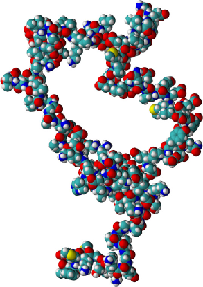
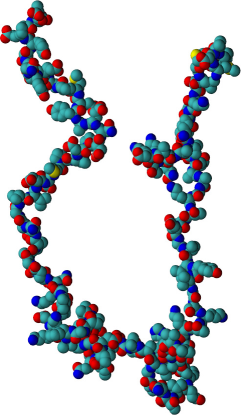
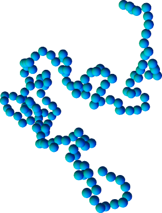
Figure 2: Snapshots of the (left) all-atom, (center) united-atom, and (right) coarse-grained representations of $\alpha$-synuclein from Langevin dynamics simulations at temperature $T_{0}=293{\rm K}$, pH $7.4$, and ratio of hydrophobic to electrostatic interactions $\alpha=1.1$. For the all-atom and united-atom models, hydrogen, carbon, oxygen, nitrogen, and sulfur atoms are colored white, cyan, red, blue, and yellow, respectively. For the coarse-grained model, each blue-shaded monomer represents an amino acid.

All-Atom Model

The all-atom model (including hydrogen atoms) matches closely the geometric properties of proteins. The average bond lengths $\langle l_{ij}\rangle$, bond angles $\langle\theta_{ijk}\rangle$, and backbone dihedral angle $\omega$ between atoms $C_{\alpha}$-$C$-$N$-$C_{\alpha}$ on successive residues were obtained from the Dunbrack database of $850$ high-resolution protein crystal structures [13]. The $242$ distinct bonds and $440$ distinct bond angles in $\alpha$-synuclein were fixed using the following spring potentials:

$$V^{bl}=\frac{k_{l}}{2}\sum_{ij}(r_{ij}-\langle l_{ij}\rangle)^{2},$$ (1)

where $k_{l}$ is the bond-length stiffness and $r_{ij}$ is the center-to-center separation between bonded atoms $i$ and $j$, and

$$V^{ba}=\frac{k_{\theta}}{2}\sum_{ijk}(\theta_{ijk}-\langle\theta_{ijk}\rangle)^{2},$$ (2)

where $k_{\theta}$ is the bond-angle stiffness and $\theta_{ijk}$ is the angle between bonded atoms $i$, $j$, and $k$. The average backbone dihedral angle between the $C_{\alpha}$-$C$-$N$-$C_{\alpha}$ atoms was constrained to zero using

$$V^{da}=\frac{k_{\omega}}{2}\sum_{ijkl}\omega_{ijkl}^{2}.$$ (3)

We chose $k_{l}=5\times 10^{3}\leavevmode\nobreak\ k_{b}T_{0}/\mbox{Å}^{2}$ and $k_{\theta}=k_{\omega}=2\times 10^{5}\leavevmode\nobreak\ k_{b}T_{0}/{\rm rad}^{2}$ (with $T_{0}=293{\rm K}$) so that the root-mean-square (rms) fluctuations in the bond lengths, bond angles, and dihedral angles were below $0.05\leavevmode\nobreak\ \mbox{Å}$ and $0.008\leavevmode\nobreak\ {\rm rad}$, respectively. These rms values occur in the protein crystal structures from the Dunbrack database. Note that no explicit interaction potentials were used to constrain the backbone dihedral angles $\phi$ and $\psi$ and side-chain dihedral angles. However, the bond lengths, bond angles, and sizes of the atoms were were calibrated so that they take on physical values. (See Appendix A.)

We included three types of interactions between nonbonded atoms: 1) the purely repulsive Lennard-Jones potential $V^{r}$ to model steric interactions, 2) attractive Lennard-Jones interactions $V^{a}$ between $C_{\alpha}$ atoms on each residue to model hydrophobicity, and 3) screened electrostatic interactions $V^{es}$ between atoms in the charged residues LYS, ARG, HIS, ASP, and GLU. Thus, the total interaction energy is $V=V^{bl}+V^{ba}+V^{da}+V^{r}+V^{a}+V^{es}$. (See Fig. 3.)

The purely repulsive Lennard-Jones potential is

$$V^{r}=\epsilon_{r}\left(4\left[\left(\frac{\sigma_{ij}^{r}}{r_{ij}}\right)^{12}-\left(\frac{\sigma_{ij}^{r}}{r_{ij}}\right)^{6}\right]+1\right)\\ \times\Theta\left(2^{1/6}\sigma_{ij}^{r}-r_{ij}\right),$$ (4)

where $\Theta\left(x\right)$ is the Heaviside step function that sets $V^{r}=0$ for $r_{ij}\geq 2^{1/6}\sigma^{r}_{ij}$, $\epsilon_{r}/k_{b}T_{0}=1$, and $\sigma_{ij}^{r}=(\sigma_{i}^{r}+\sigma_{j}^{r})/2$ is the average diameter of atoms $i$ and $j$. We used the atom sizes (for hydrogen, carbon, oxygen, nitrogen, and sulfur) from Ref. [14] after verifying that the backbone dihedral angles for the all-atom model sample the sterically allowed $\phi$ and $\psi$ values in the Ramachandran map [15] when $V=V^{bl}+V^{ba}+V^{da}+V^{r}$. (See Appendix A.)

The hydrophobic interactions between residues were modeled using the attractive Lennard-Jones potential

$$V^{a}=\epsilon_{a}\sum_{ij}\left[\lambda_{ij}\left(4\left[\left(\frac{\sigma^{a}}{R_{ij}}\right)^{12}-\left(\frac{\sigma^{a}}{R_{ij}}\right)^{6}\right]+1\right)\right.\\ \left.\times\Theta\left(R_{ij}-2^{1/6}\sigma^{a}\right)-\lambda_{ij}\right],$$ (5)

where $\epsilon_{a}$ is the attraction strength, $R_{ij}$ is the center-to-center separation between $C_{\alpha}$ atoms on residues $i$ and $j$,

$$\lambda_{ij}=\sqrt{h_{i}h_{j}},$$ (6)

$h_{i}$ is the hydrophobicity index for residue $i$ that ranges from $0$ (hydrophilic) to $1$ (hydrophobic) in Table  1, and $\sigma^{a}\approx 4.8\leavevmode\nobreak\ \mbox{Å}$ is the typical separation between centers of mass of neighboring residues. We find that the results for the conformational statistics for $\alpha$-synuclein are not sensitive to small changes in $\sigma^{a}$ and $h_{i}$ (Appendix B).

The screened Coulomb potential was used to model the electrostatic interactions between atoms $i$ and $j$ for $\alpha$-synuclein in water:

$$V^{es}=\epsilon_{es}\sum_{ij}\frac{q_{i}q_{j}}{e^{2}}\frac{\sigma^{a}}{r_{ij}}e^{-\frac{r_{ij}}{\ell}},$$ (7)

where $e$ is the fundamental charge, $\epsilon_{es}=\sigma^{a}e^{2}/4\pi\epsilon_{0}\epsilon$, $\epsilon_{0}$ is the vacuum permittivity, $\epsilon=80$ is the permittivity of water, and $\ell=9\leavevmode\nobreak\ \mbox{Å}$ is the Coulomb screening length in an aqueous solution with a $150{\rm mM}$ salt concentration. The partial charge $q_{i}$ on atom $i$ in one of the charged residues LYS, ARG, HIS, ASP, and GLU is given in Table 2.

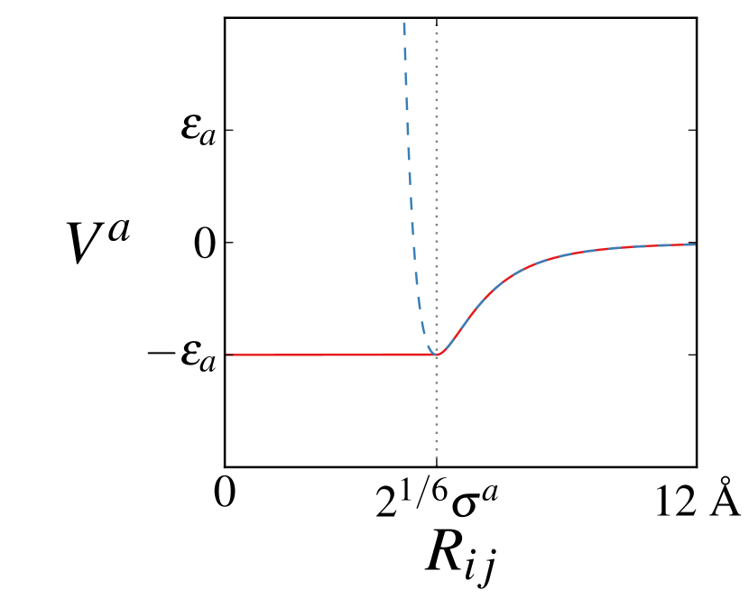
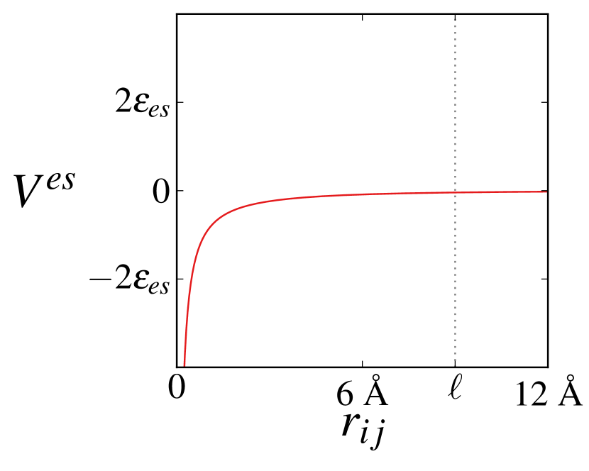
Figure 3: Schematics of (a) the purely repulsive Lennard-Jones potential $V^{r}$ in Eq. 4 (solid line), (b) attractive Lennard-Jones potential $V^{a}$ in Eq. 5 (solid line), and (c) screened Coulomb potential $V^{es}$ in Eq. 7 (solid line). The dashed line in (b) represents repulsive Lennard-Jones interactions between residues $i$ and $j$ in the coarse-grained model.

ALA	ARG	ASN	ASP	CYS	GLN	GLU	GLY	HIS	ILE
0.735	0.37	0.295	0.41	0.76	0.41	0.54	0.5	0.29	1
LEU	LYS	MET	PHE	PRO	SER	THR	TRP	TYR	VAL
0.985	0.385	0.87	1	0.27	0.475	0.565	0.985	0.815	0.88

Table 1: Hydrophobicity indices $h_{i}$ that range from $0$ (hydrophilic) to $1$ (hydrophobic) for residues in $\alpha$-synuclein at pH $7.4$ [16].

Residue	Atom	Atom Charge $q_{i}$	Residue Charge $Q_{i}$
LYS	$\ce{N_{\zeta}}$	1	1
ARG	$\ce{N_{\eta 1}}$	0.39	1
	$\ce{N_{\eta 2}}$	0.39
	$\ce{N_{\varepsilon}}$	0.22
HIS	$\ce{N^{\delta 1}}$	0.05	0.1
	$\ce{N^{\varepsilon 2}}$	0.05
ASP	$\ce{O^{\delta 1}}$	-0.5	-1
	$\ce{O^{\delta 2}}$	-0.5
GLU	$\ce{O^{\varepsilon 1}}$	-0.5	-1
	$\ce{O^{\varepsilon 2}}$	-0.5

Table 2: Partial charges $q_{i}$ on atom $i$ (left) and total charge $Q_{i}$ on residue $i$ (right) for the charged residues LYS, ARG, HIS, ASP, and GLU at pH $7.4$ [17]. The total partial charge $q=\sum_{i}q_{i}$ for the N-terminal, central, and C-terminal regions are $4.1$, $-1$, and $-12.0$, respectively.

United-Atom Model

For the united-atom model, we do not explicitly model the hydrogen atoms. Instead, we use a set of $11$ atom sizes $\sigma_{i}^{r}$ from Ref. [18], where the hydrogens are subsumed into the heavy atoms: C ($\sigma_{i}^{r}/2=1.53\leavevmode\nobreak\ \mbox{Å}$), CH ($1.80\leavevmode\nobreak\ \mbox{Å}$), C${\rm H}_{2}$ ($1.80\leavevmode\nobreak\ \mbox{Å}$), C${\rm H}_{3}$ ($1.80\leavevmode\nobreak\ \mbox{Å}$), O ($1.26\leavevmode\nobreak\ \mbox{Å}$), OH ($1.44\leavevmode\nobreak\ \mbox{Å}$), N ($1.53\leavevmode\nobreak\ \mbox{Å}$), N${\rm H}_{2}$ ($1.57\leavevmode\nobreak\ \mbox{Å}$), N${\rm H}_{3}$ ($1.80\leavevmode\nobreak\ \mbox{Å}$), and S ($1.62\leavevmode\nobreak\ \mbox{Å}$). We optimized the atom sizes by characterizing the backbone dihedral angles $\phi$ and $\psi$ as a function of $\sigma_{i}^{r}$ in the united-atom simulations with $V=V^{bl}+V^{ba}+V^{da}+V^{r}$. The $\phi$ and $\psi$ backbone dihedral angle distributions closely match that from the Ramachandran map (i.e. the $\alpha$-helix and $\beta$-sheet regions) when we scale the atom sizes in Ref. [18] by $0.9$ as shown in Appendix  A. Otherwise, the all-atom and united-atom models use the same interaction potentials in Eqs. 1-7.

Coarse-Grained Model

For the coarse-grained model, we employed a backbone-only $C_{\alpha}$ representation of $\alpha$-synuclein where each residue $i$ is represented by a spherical monomer $i$ with size $\sigma^{a}$, mass $M$, hydrophobicity $h_{i}$, and charge $Q_{i}$. The average bond length between monomers $i$ and $j$ was fixed to $\langle l_{ij}\rangle=4.0\leavevmode\nobreak\ \mbox{Å}$, which is the average separation between $C_{\alpha}$ atoms on neighboring residues, using Eq. 1 (with $r_{ij}$ replaced by $R_{ij}$). The bond-angle $\Theta$ (between three successive $C_{\alpha}$ atoms) and dihedral-angle $\Phi$ (between four successive $C_{\alpha}$ atoms) potentials were calculated so that the $\Theta$ and $\Phi$ distributions matched those from the united-atom simulations with $V=V^{bl}+V^{ba}+V^{da}+V^{r}$. The $\Theta$ distributions from the united-atom model were approximately Gaussian with mean $\langle\Theta\rangle=2.13\leavevmode\nobreak\ {\rm rad}$ and standard deviation $\sigma_{\Theta}=0.345\leavevmode\nobreak\ {\rm rad}$.

The dihedral angle potential $V^{da}$ for the coarse-grained simulations was obtained by fitting the distribution $P(\Phi)$ from the united-atom simulations to a seventh-order Fourier series

$$V^{da}(\Phi) = \sum_{k=0}^{6}a_{k}\cos\left(k\Phi\right)+b_{k}\sin\left(k\Phi\right),$$

where $a_{k}=-2k_{b}T_{0}\left\langle\cos\left(k\Phi\right)\log P\left(\Phi\right)\right\rangle$, $b_{k}=-2k_{b}T_{0}\left\langle\sin\left(k\Phi\right)\log P\left(\Phi\right)\right\rangle$, and the angle brackets indicate an average over time and dihedral angles along the protein backbone.

For steric interactions between residues, we used the purely repulsive Lennard-Jones potential in Eq. 4 with $r_{ij}$ and $\sigma^{r}_{ij}$ replaced by $R_{ij}$ and $\sigma^{a}$ respectively. The hydrophobic interactions are the same as those in Eqs. 5 and 6 with $\epsilon_{a}=\epsilon_{r}$. The electrostatic interactions between residues are given by Eq. 7 with $q_{i}$ and $r_{ij}$ replaced by $Q_{i}$ and $R_{ij}$, respectively.

Langevin Dynamics

The all-atom, united-atom, and coarse-grained models were simulated at fixed $NVT$ using a Langevin thermostat [19], modified velocity Verlet integration scheme, and free boundary conditions. We set the time step $\Delta t=10^{-2}t_{0}$ and damping coefficient $\gamma=10^{-3}t_{0}^{-1}$, where $t_{0}=\sqrt{m\langle\sigma_{ij}^{r}\rangle/\epsilon_{r}}$ and $m$ is the hydrogen mass for the all-atom and united-atom models and $t_{0}=\sqrt{M\sigma^{a}/\epsilon_{r}}$ for the coarse-grained model. The initial atomic positions were obtained from a micelle-bound NMR structure (protein data bank identifier 1XQ8) for $\alpha$-synuclein at pH $7.4$ and temperature $298{\rm K}$ [20]. The initial positions for the coarse-grained model were obtained from simulations at high temperature with only bond-length, bond-angle, and dihedral-angle constraints and repulsive Lennard-Jones interactions. The simulations were run for times much longer than the characteristic relaxation time from the decay of the radius of gyration autocorrelation function.

In the results below, we will study the radius of gyration $R_{g}$ and distribution of inter-residue separations $P(R_{ij})$ as a function of the ratio of the attractive hydrophobic and electrostatic energy scales $\alpha=\epsilon_{a}/\epsilon_{es}$ and quantitatively compare the results from smFRET experiments and all-atom, united-atom, and coarse-grained simulations.

3 Results

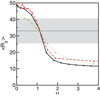
Figure 4: Average radius of gyration $\langle R_{g}\rangle$ versus the ratio of the attractive hydrophobic to electrostatic interactions $\alpha$ for the coarse-grained (black solid), united-atom (red dashed), and all-atom (green dotted) models at $T_{0}$ (or the temperature that gives $R_{g}\approx 33\leavevmode\nobreak\ \mbox{Å}$ in the coarse-grained simulations) and pH $7.4$. The horizontal line and gray shaded region indicate the average and standard deviation over recent NMR, SAXS, and smFRET experimental measurements, $\langle R_{g}\rangle=33.0\pm 7.7\leavevmode\nobreak\ \mbox{Å}$, for monomeric $\alpha$-synuclein near $T_{0}$ and neutral pH [4, 7, 9, 12, 21, 22, 23, 24].

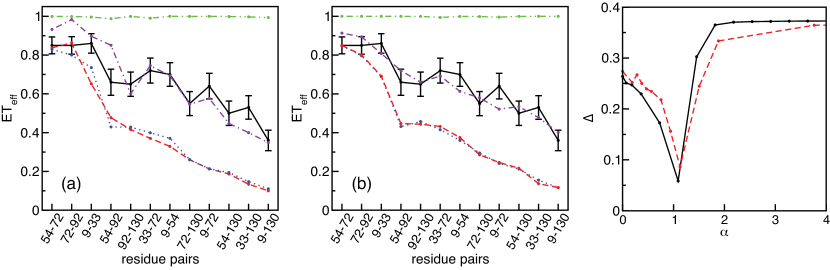
Figure 5: A comparison of FRET efficiencies $ET_{\textrm{eff}}$ for twelve residue pairs from simulations and experiments of $\alpha$-synuclein. In (a) the data includes FRET efficiencies from united-atom simulations of a random walk (red dashed), collapsed globule (green dot-dot-dashed), only electrostatic interactions at temperature $T_{0}$ (blue dotted), and ratio of attractive hydrophobic to electrostatic interactions $\alpha=1.1$ (purple dot-dashed) at $T_{0}$ and recent smFRET experiments [12] (black solid). Error bars from experiments were calculated using a resampling method that accounts for uncertainty in the determination of $ET_{\rm eff}$ ($1$-$2\%$) and variations in $R_{0}$ ($7$-$8\%$) due to the effects of the protein environment on the smFRET fluorophores. In (b) we compare the FRET efficiencies from recent smFRET experiments [12] to the coarse-grained simulations of a random walk (red dashed), collapsed globule (green dot-dot-dashed), only electrostatics interactions (blue dotted), and both attractive hydrophobic and electrostatic interactions with $\alpha=1.1$ at a temperature that yields $\langle R_{g}\rangle\approx 33\leavevmode\nobreak\ \mbox{Å}$ (purple dot-dashed). (c) The rms deviation $\Delta$ between the FRET efficiencies from the united-atom simulations and smFRET experiments (black solid) and the coarse-grained simulations and smFRET experiments (red dashed) versus $\alpha$. The minimum rms $\Delta_{\rm min}\approx 0.09$ occurs near $\alpha\approx 1.1$ for both the united-atom and coarse-grained simulations.

In Fig. 4, we show the radius of gyration that characterizes the overall protein shape for the all-atom, united-atom, and coarse-grained models,

$$R_{g}=\sqrt{\frac{1}{N}\sum_{i=1}^{N}({\vec{r}}_{i}-\langle{\vec{r}}_{i}\rangle)^{2}},$$ (8)

where ${\vec{r}}_{i}$ is the position of atom or monomer $i$, as a function of the ratio of the attractive hydrophobic to electrostatic interactions $\alpha$ at temperature $T_{0}$ and pH $7.4$. For $\alpha\gg 1$, the protein forms a collapsed globule with $\langle R_{g}\rangle\approx 12$-$15\leavevmode\nobreak\ \mbox{Å}$. Whereas for $\alpha\ll 1$, the models only include electrostatics interactions, and $\langle R_{g}\rangle$ is similar to the random walk values for the three models (all-atom: $42.8\leavevmode\nobreak\ \mbox{Å}$, united-atom: $48.6\leavevmode\nobreak\ \mbox{Å}$, coarse-grained: $48.2\leavevmode\nobreak\ \mbox{Å}$). The crossover between random walk and collapsed globule behavior for $\langle R_{g}\rangle$ occurs near $\alpha\approx 1$.

A number of recent SAXS, NMR, and smFRET experiments have measured the radius of gyration for monomeric $\alpha$-synuclein near $T_{0}$ and neutral pH [4, 7, 9, 12, 21, 22, 23, 24]. As shown in Fig. 4, the average over these experimental measurements is $\langle R_{g}\rangle=33.0\pm 7.7\leavevmode\nobreak\ \mbox{Å}$, and thus the $\langle R_{g}\rangle$ for $\alpha$-synuclein falls in between the random walk and collapsed globule values.

We can more quantitatively compare simulation and experimental studies of $\alpha$-synuclein by calculating the distributions of inter-residue distances or, equivalently, the FRET efficiencies. FRET efficiencies between residues $i$ and $j$ are obtained from

$$ET_{\rm eff}=\left\langle\frac{1}{1+\left(\frac{R_{ij}}{R_{0}}\right)^{6}}\right\rangle,$$ (9)

where $R_{0}=54\leavevmode\nobreak\ \mbox{Å}$ is the Förster distance for the fluorophore pair in Refs. [11, 25] and the angle brackets indicate an average over time. To calculate $\langle R_{ij}\rangle$ from the FRET efficiencies, one must invert Eq. 9 using the distribution of inter-residue separations $P(R_{ij})$.

The FRET efficiencies for the twelve residue pairs from recent smFRET experiments on $\alpha$-synuclein [11] and the united-atom and coarse-grained simulations are shown in Fig. 5 (a) and (b). Errors in the inter-residue separation distributions can occur in both the directly measured $ET_{\rm eff}$ values and $R_{0}$. To estimate the errors, we generated $10$ decoy sets of inter-residue separations using $ET_{\rm eff}$ and $R_{0}$ values drawn from distributions accounting for the individual uncertainties. We then calculated the rms deviation over each decoy set assuming that we know $R_{0}$ precisely.

We identify several important features in the comparison of the FRET efficiencies from experiments and simulations in Fig. 5 (a) and (b): 1) The united-atom and coarse-grained models yield qualitatively similar results for the FRET efficiencies; 2) The FRET efficiencies for the random walk and pure electrostatics models are similar to each other and much lower than most of the residue pair FRET efficiencies from experiments; 3) The FRET efficiencies for the collapsed globule $\approx 1$ and do not match those from experiments; and 4) By tuning $\alpha$, we are able to match quantitatively the FRET efficiencies from the experiments and simulations.

As shown in Fig. 5 (c), the rms deviations $\Delta$ between the FRET efficiencies from the united-atom simulations and smFRET experiments and between the FRET efficiencies from the coarse-grained simulations and smFRET experiments are minimized when $\alpha\approx 1.1$. For the united-atom model, $\alpha\approx 1.1$ gives $\langle R_{g}\rangle\approx 33\leavevmode\nobreak\ \mbox{Å}$, which is similar to that found in Ref. [12]. The largest deviations in the FRET efficiencies between the united-atom simulations and smFRET experiments occur for small inter-residue separations, which are likely caused by the finite size of the dye molecules. Note that the deviations at small inter-residue separations are much weaker for the coarse-grained simulations. Thus, we find that it is crucial to include both electrostatic and attractive hydrophobic interactions in modeling $\alpha$-synuclein in solution.

For the coarse-grained simulations, we also studied the variation of the FRET efficiencies as a function of temperature (not only at $T=T_{0}$). In Fig. 6, we show the rms deviation between the FRET efficiencies for the coarse-grained simulations and smFRET experiments for the twelve residue pairs considered in Ref. [12] as a function of $\alpha$ and $k_{b}T/\epsilon_{r}$. We find that the line of $\alpha$ and $k_{b}T/\epsilon_{r}$ values that give $\langle R_{g}\rangle\simeq 33\leavevmode\nobreak\ \mbox{Å}$ lies in the region where the rms deviations in the FRET efficiencies are minimized, which indicates that there is a class of polymeric structures with similar conformational statistics to that of $\alpha$-synuclein.

In Fig. 7, we compare the inter-residue separation distributions $P(R_{ij})$ obtained from experimentally constrained Monte Carlo (ECMC) and united-atom (with $\alpha=1.1$) simulations. For the ECMC simulations discussed in detail in Ref. [12], we assumed that $P(R_{ij})$ was similar to that for a random walk $C_{\alpha}$ model with only bond-length, bond-angle, and dihedral-angle ($\omega$) constraints and repulsive Lennard-Jones interactions to obtain $\langle R_{ij}\rangle$ from the experimentally measured FRET efficiencies. We find that $\langle R_{ij}\rangle$ for the ECMC and united-atom simulations agree to within roughly $10\%$ (Fig. 8 (left)), however, the standard deviations differ significantly, as shown in Fig. 8 (right). The standard deviation of $P(R_{ij})$ for the united-atom simulations is larger than that for the ECMC simulations for all residue pairs and scales as $\sigma_{R}\sim|i-j|^{\delta}$ with $\delta\sim 0.6$ (compared to the excluded volume random walk scaling exponent $\delta=0.69$). Further, $\sigma_{R}$ for residue pairs that are not constrained in ECMC do not obey the scaling behavior with $i-j$ as found for residue pairs that were constrained ($\sigma_{R}\sim|i-j|^{\delta}$ with $\delta\sim 0.4$ [12]).

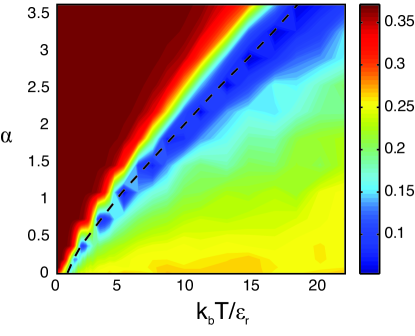
Figure 6: RMS deviations $\Delta$ between the coarse-grained and experimental FRET efficiencies for the twelve residue pairs considered in Ref.[12] as a function of $\alpha$ and $k_{b}T/\epsilon_{r}$. The dashed line indicates systems that give $\langle R_{g}\rangle\simeq 33\leavevmode\nobreak\ \mbox{Å}$. Note that this line coincides with the minimum values for the rms deviations.

Figure 7: Probability distributions for the inter-residue separations $P(R_{ij})$ for the twelve residue pairs considered in Ref. [12] and eleven additional pairs for experimentally constrained Monte Carlo (ECMC) [12] (left) and united-atom (with $\alpha=1.1$; right) simulations. The average inter-residue separations $\langle R_{ij}\rangle$ for the united atom and ECMC simulations are shown with solid and dashed lines, respectively.

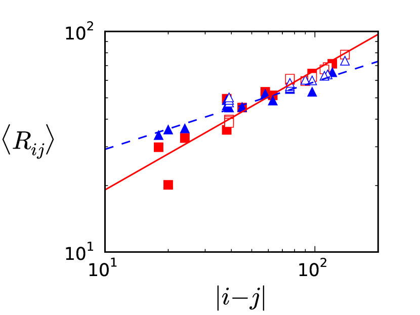
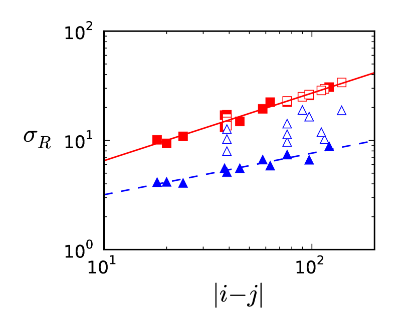
Figure 8: Average $\langle R_{ij}\rangle$ and standard deviation $\sigma_{R}$ of the inter-residue separation distributions in Fig. 7 for the united-atom (squares) and ECMC (triangles) simulations versus chemical distance between residues $|i-j|$. The filled symbols indicate residue pairs that were considered in smFRET experiments [12] and open symbols indicate other pairs. The solid and dashed lines have slopes $0.54$ and $0.31$ (left panel) and $0.62$ and $0.38$ (right panel), respectively.

4 Conclusions and Future Directions

We have shown that we are able to accurately model the conformational dynamics (i.e. the inter-residue separations) of the IDP $\alpha$-synuclein at temperature $T_{0}=293{\rm K}$ and neutral pH using all-atom, united-atom, and coarse-grained Langevin dynamics simulations. Our results show that the structure of $\alpha$-synuclein is intermediate between that for random walks and collapsed globules with the rms separation $\sigma_{R}$ between residues $i$ and $j$ scaling as $|i-j|^{\delta}$ with $\delta\sim 0.6$. The calibrated Langevin dynamics simulations presented here have the advantage over constraint methods in that physical forces act on all residues, not only on residue pairs that are monitored experimentally, and can be tuned to match FRET efficiencies from experiments. In future work, we will employ calibrated Langevin dynamics simulations to study the conformational dynamics of $\alpha$-synuclein at low pH and the interaction and association between two or more $\alpha$-synuclein monomers as a function of pH to identify mechanisms for $\alpha$-synuclein oligomerization. In preliminary calibrated coarse-grained Langevin dynamics simulations, we find that two monomeric $\alpha$-synuclein proteins only associate for sufficiently strong attractive hydrophobic interactions ($\alpha\geq 1.1$), as shown in Fig. 9.

Figure 9: Snapshots from preliminary aggregation studies of two monomeric $\alpha$-synuclein proteins (dark green and light blue) using coarse-grained simulations with the temperature set so that $\langle R_{g}\rangle\approx 33\leavevmode\nobreak\ \mbox{Å}$ at $\alpha=1.1$ (for individual protein monomers) for (a) $\alpha=0.7$ (b) $1.1$, (c) $1.3$, (d) $1.5$, and (e) $1.8$.

5 Acknowledgments

This research was supported by the National Science Foundation under Grant Nos. DMR-1006537 (CO, CS), PHY-1019147 (WS), BIO-0919853 (ER), and the Raymond and Beverly Sackler Institute for Biological, Physical, and Engineering Sciences (CO, ER). This work also benefited from the facilities and staff of the Yale University Faculty of Arts and Sciences High Performance Computing Center and NSF Grant No. CNS-0821132 that partially funded acquisition of the computational facilities.

Appendix A Calibration of Atom Sizes

In this Appendix, we test the choice of the atom sizes used in the all-atom and united-atom models by measuring the Ramachandran plot [15] for the backbone dihedral angles $\phi$ and $\psi$. In Fig. 10, we show that the Ramachandran plot for the random walk all-atom model of $\alpha$-synuclein with no attractive hydrophobic and electrostatic interactions and atom sizes from Ref. [14] closely resembles that for dipeptides with highly populated $\alpha$-helix and $\beta$-sheet regions. In Fig. 11, we show the Ramachandran plots for the backbone dihedral angles $\phi$ and $\psi$ obtained from the random walk united-atom model of $\alpha$-synuclein with no attractive hydrophobic and electrostatic interactions and atom sizes $0.8$, $0.85$, $0.9$, $0.95$, and $1.0$ times those from Ref. [18]. We find that the Ramachandran plot for united-atom model with a factor of $0.9$ for the atom sizes is similar to that for the all-atom model.

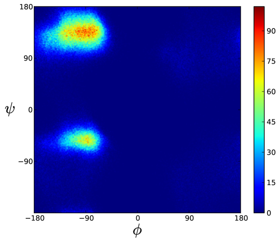
Figure 10: Ramachandran plot for the backbone dihedral angles $\phi$ and $\psi$ obtained from the all-atom random walk simulations with no attractive hydrophobic and electrostatic interactions, and atom sizes given in Ref. [14]. The highly populated $\phi$ and $\psi$ angles indicate $\beta$-sheet (upper left) and $\alpha$-helix (lower left) conformations.

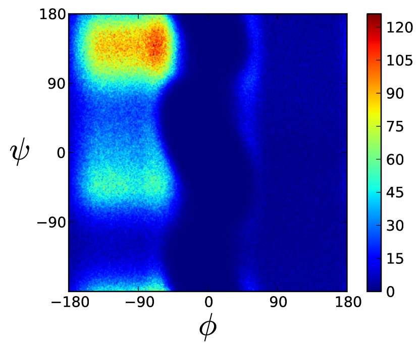
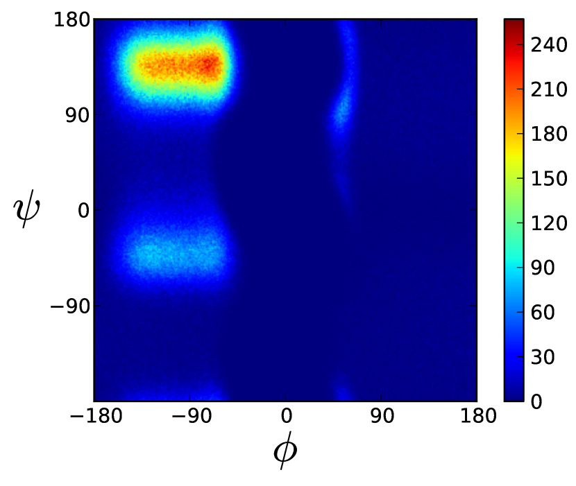
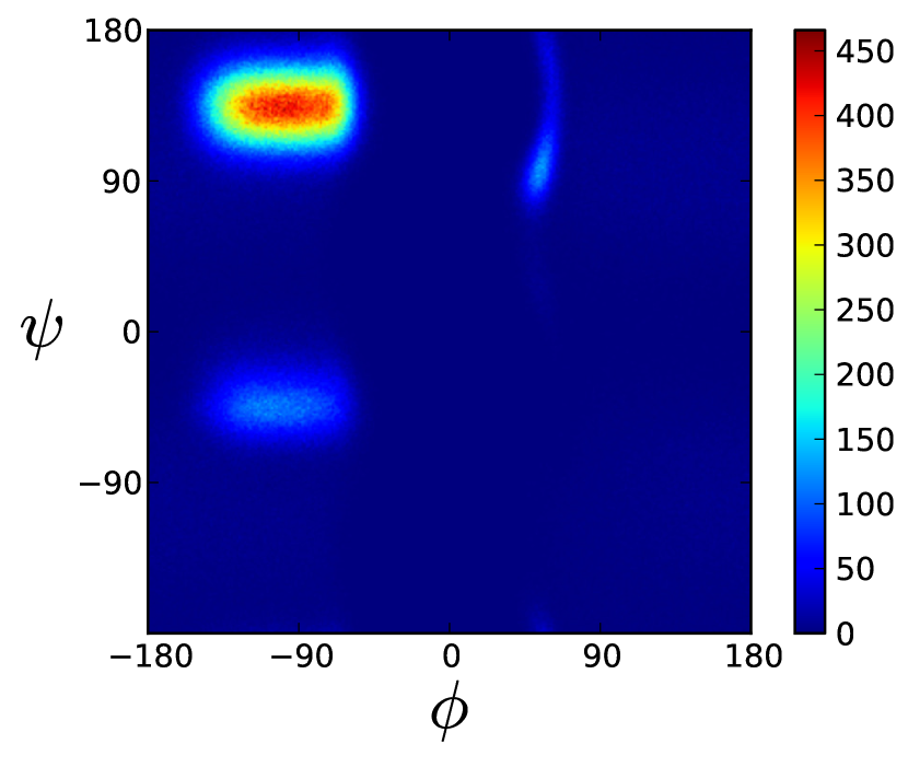
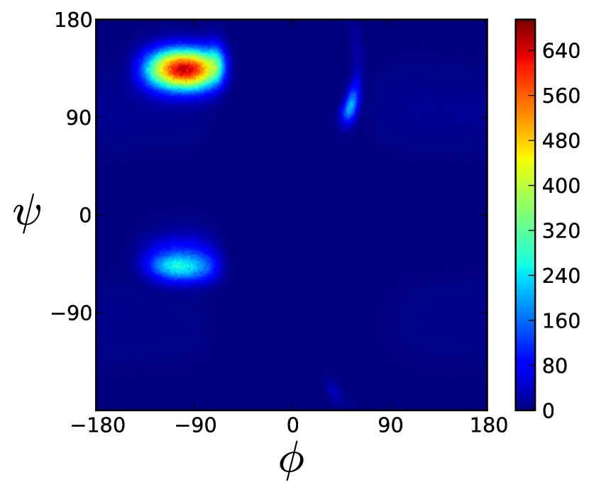
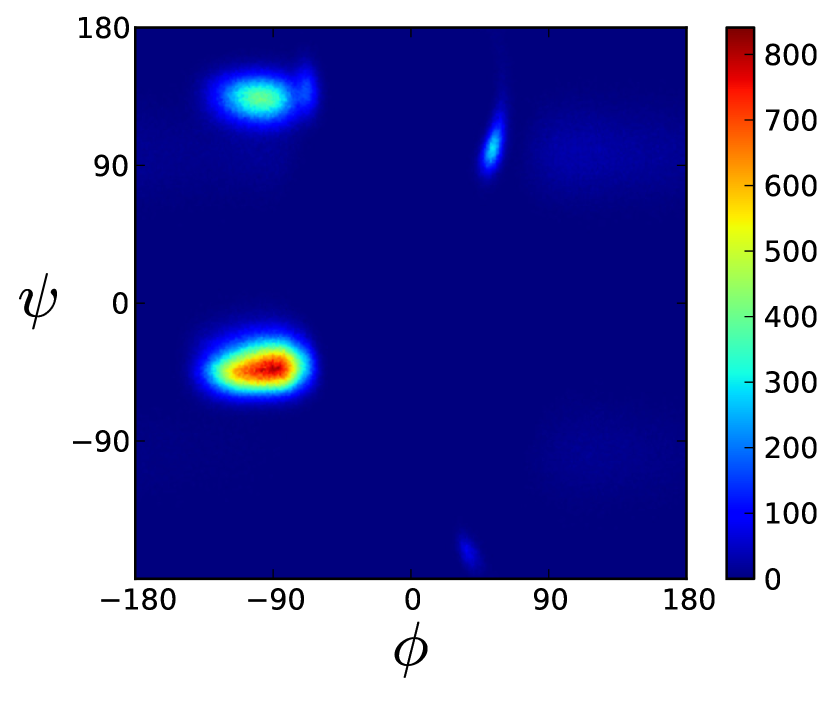
Figure 11: Ramachandran plot for the backbone dihedral angles $\phi$ and $\psi$ obtained from the united-atom random walk simulations with no attractive hydrophobic and electrostatic interactions and atom sizes $0.8$ (upper left), $0.85$ (upper right), $0.9$ (middle left), $0.95$ (middle right), and $1.0$ (bottom) times those given in Ref. [18].

Appendix B Robustness of the Hydrophobic Interactions

In this Appendix, we study the sensitivity of the FRET efficiencies for the united-atom simulations to small variations in the lengthscale $\sigma^{a}$ above which the attractive hydrophobic interactions are nonzero and relative strengths $h_{i}$ of the attractive hydrophobic interactions for different residues. In Fig. 12 (left), we show that the FRET efficiencies for the twelve residue pairs show only small variations with $\sigma^{a}$ over the range from $4.3\leavevmode\nobreak\ \mbox{Å}$ to $5.2\leavevmode\nobreak\ \mbox{Å}$ (except for $9$-$72$ with $\sigma^{a}=4.3\leavevmode\nobreak\ \mbox{Å}$). In Fig. 12 (right), we show that the FRET efficiencies for the twelve residue pairs are robust for $\Delta h<0.5$.

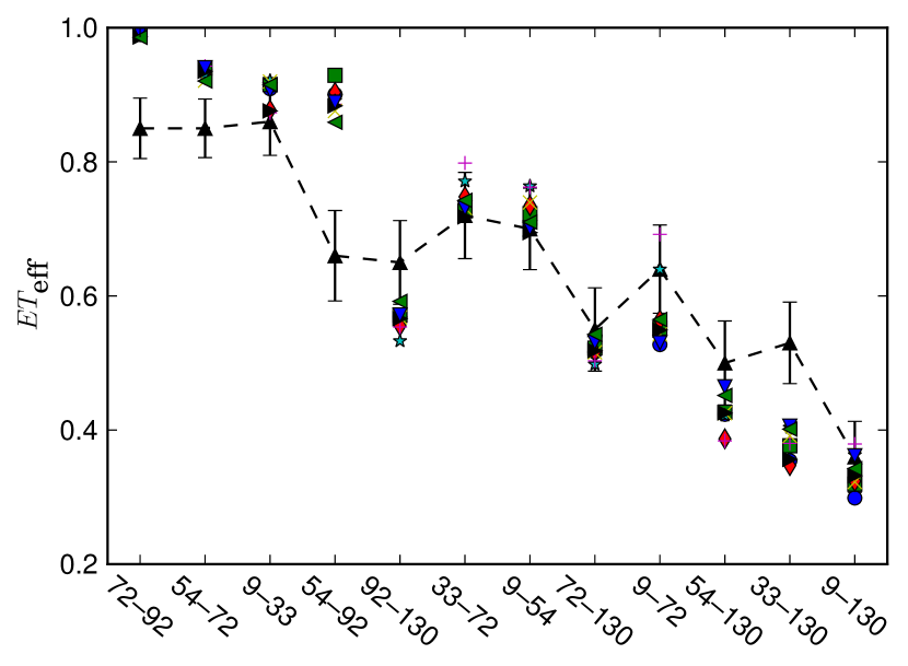
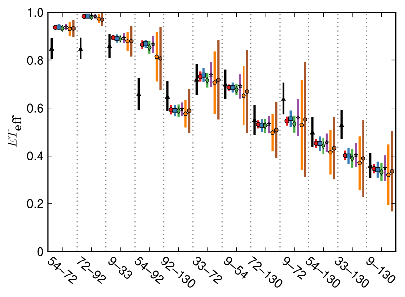
Figure 12: (left) FRET efficiencies $ET_{\rm eff}$ for the twelve residue pairs considered in Ref. [12] from smFRET experiments (upward triangles) and united-atom simulations with $\alpha$ set so that $R_{g}\approx 33\leavevmode\nobreak\ \mbox{Å}$ and $\sigma^{a}=4.4\leavevmode\nobreak\ \mbox{Å}$ (circles), $4.6\leavevmode\nobreak\ \mbox{Å}$ (squares), $4.8\leavevmode\nobreak\ \mbox{Å}$ (diamonds), $5.0\leavevmode\nobreak\ \mbox{Å}$ (stars), and $5.2\leavevmode\nobreak\ \mbox{Å}$ (pentagons). (right) FRET efficiencies $ET_{\rm eff}$ for the twelve residue pairs considered in Ref. [12] for the united-atom simulations for $\alpha=1.1$ and varying hydrophobicity indices $h_{i}^{\prime}=h_{i}+\Delta h$, where $\Delta h$ is chosen from a zero-mean Gaussian distribution with standard deviation $0.0$ (circles), $0.02$ (squares), $0.05$ (diamonds), $0.05$ (diamonds), $0.1$ (stars), $0.3$ (pentagons), $0.5$ (hexagons). The average $ET_{\rm eff}$ and its standard deviation for $32$ samples are shown for each $\Delta h$.

References

- [1] Vucetic, S.; Brown, C. J.; Dunker, A. K.; Obradovic, Z. Proteins: Structure, Function, and Bioinformatics 2003, 52, 573–584.
- [2] Sugase, K.; Dyson, H. J.; Wright, P. E. Nature 2007, 447, 1021–1025.
- [3] Uversky, V. N.; Oldfield, C. J.; Dunker, A. K. Annu. Rev. Biophys. 2008, 37, 215–246.
- [4] Dedmon, M. M.; Lindorff-Larsen, K.; Christodoulou, J.; Vendruscolo, M.; Dobson, C. M. J. Am. Chem. Soc. 2004, 127, 476–477.
- [5] Vilar, M.; Chou, H.-T.; Lührs, T.; Maji, S. K.; Riek-Loher, D.; Verel, R.; Manning, G.; Stahlberg, H.; Riek, R. Proceedings of the National Academy of Sciences 2008, 105, 8637–8642.
- [6] Eliezer, D.; Kutluay, E.; Bussell Jr, R.; Browne, G. Journal of Molecular Biology 2001, 307, 1061–1073.
- [7] Li, J.; Uversky, V. N.; Fink, A. L. NeuroToxicology 2002, 23, 553–567.
- [8] Tsigelny, I. F.; Bar-On, P.; Sharikov, Y.; Crews, L.; Hashimoto, M.; Miller, M. A.; Keller, S. H.; Platoshyn, O.; Yuan, J. X. J.; Masliah, E. FEBS Journal 2007, 274, 1862–1877.
- [9] Uversky, V. N.; Yamin, G.; Munishkina, L. A.; Karymov, M. A.; Millett, I. S.; Doniach, S.; Lyubchenko, Y. L.; Fink, A. L. Molecular Brain Research 2005, 134, 84–102.
- [10] Ullman, O.; Fisher, C. K.; Stultz, C. M. Journal of the American Chemical Society 2011, 133, 19536–19546.
- [11] Trexler, A. J.; Rhoades, E. Biophysical Journal 2010, 99, 3048–3055.
- [12] Nath, A.; Sammalkorpi, M.; DeWitt, D. C.; Trexler, A. J.; S., E.-G.; O’Hern, C. S.; Rhoades, E. Biophysical Journal 2012, To appear.
- [13] Dunbrack Jr., R. L.; Cohen, F. E. Protein Science 1997, 6, 1661–1681.
- [14] Zhou, A. Q.; O’Hern, C. S.; Regan, L. Biophysical Journal 2012, 102, 2345–2352.
- [15] Ramachandran, G.; Ramakrishnan, C.; Sasisekharan, V. Journal of Molecular Biology 1963, 7, 95 – 99.
- [16] Monera, O. D.; Sereda, T. J.; Zhou, N. E.; Kay, C. M.; Hodges, R. S. Journal of Peptide Science 1995, 1.
- [17] Oostenbrink, C.; Villa, A.; Mark, A. E.; Van Gunsteren, W. F. Journal of Computational Chemistry 2004, 25, 1656–1676.
- [18] Richards, F. Journal of Molecular Biology 1974, 82, 1–14.
- [19] Ermak, D. L.; Buckholz, H. Journal of Computational Physics 1980, 35, 169 – 182.
- [20] Ulmer, T. S.; Bax, A.; Cole, N. B.; Nussbaum, R. L. Journal of Biological Chemistry 2005, 280, 9595–9603.
- [21] Uversky, V. N.; Li, J.; Fink, A. L. FEBS Letters 2001, 509, 31–35.
- [22] Tashiro, M.; Kojima, M.; Kihara, H.; Kasai, K.; Kamiyoshihara, T.; Uéda, K.; Shimotakahara, S. Biochemical and Biophysical Research Communications 2008, 369, 910–914.
- [23] Rekas, A.; Knott, R.; Sokolova, A.; Barnham, K.; Perez, K.; Masters, C.; Drew, S.; Cappai, R.; Curtain, C.; Pham, C. European Biophysics Journal 2010, 39, 1407–1419.
- [24] Salmon, L.; Nodet, G.; Ozenne, V.; Yin, G.; Jensen, M. R.; Zweckstetter, M.; Blackledge, M. Journal of the American Chemical Society 2010, 132, 8407–8418.
- [25] Schuler, B.; Lipman, E. A.; Eaton, W. A. Nature 2002, 419, 743–747.