Highly anisotropic dissipative hydrodynamics

Abstract

The quark gluon plasma generated in ultrarelativistic heavy ion collisions may possess sizable momentum-space anisotropies that cause the longitudinal and transverse pressures in the local rest frame to be significantly different. We review recent attempts to derive a dynamical framework that can reliably describe systems that possess a high degree of momentum-space anisotropy. The dynamical framework that has been developed can describe the evolution of the quark gluon plasma ranging from the longitudinal free-streaming limit to the ideal hydrodynamical limit.

1 Introduction

The Relativistic Heavy Ion Collider (RHIC) and the Large Hadron Collider (LHC) are studying the behavior of nuclear matter at high energy densities, $\epsilon\gg 1\;{\rm GeV/fm}^{3}$, using relativistic heavy ion collisions. The goal of these experiments is not only to generate a deconfined quark-gluon plasma (QGP), but to also study its properties such as transport properties, color opacity, etc. One complicating factor is that the QGP generated in such collisions lasts for only a few fm/c and during this time the bulk properties of the system, e.g. energy density and pressure, can change rapidly. In addition, it is possible that in certain regimes the system is far from equilibrium/isotropy. Dynamical models that can reliably describe the evolution of the system on the fm/c timescale are necessary in order to make sound phenomenological predictions.

One of the key outstanding questions in dynamical models of the QGP is to what extent is the QGP isotropic in the local rest frame. Early indications from ideal hydrodynamical fits to experimental data for the elliptic flow of hadrons indicated that the data were consistent with isotropization at $\tau\sim 0.5$ fm/c after the initial nuclear impact Huovinen et al. (2001); Hirano and Tsuda (2002). This rather short time scale prompted a plethora of papers attempting to solve the early isotropization/thermalization puzzle. In the intervening ten years ideal hydrodynamics has been replaced by viscous hydrodynamics Israel and Stewart (1979); Muronga (2007); Luzum and Romatschke (2008); Dusling and Teaney (2008) as the method of choice for simulating the bulk dynamics of the QGP.

In viscous hydrodynamics the energy-momentum tensor in the local rest frame is naturally anisotropic with ${\cal P}_{T}\neq{\cal P}_{L}$, where ${\cal P}_{T}$ and ${\cal P}_{L}$ are the local rest frame transverse and longitudinal pressures, respectively. The relative amount of momentum-space anisotropy is encoded in the shear tensor and in viscous hydrodynamics one has the freedom to choose, in addition to initial temperature and flow profiles, an initial value for the shear profile. In the last years it has emerged that phenomenological predictions are rather insensitive to the assumed initial shear profile, see e.g. Shen et al. (2011). Further studies have shown that the period of large momentum-space anisotropy can persist for a few fm/c Ryblewski and Florkowski (2012). In addition, it can be shown that momentum-space anisotropies will be particularly large at the longitudinal and transverse edges of the plasma where the system is dilute and poorly approximated by naïve viscous hydrodynamical treatments Martinez and Strickland (2009).

In order to properly address the question of the evolution of systems that possess large momentum-space anisotropies, one needs to go beyond traditional viscous hydrodynamical treatments. Viscous hydrodynamics relies on an implicit assumption that the shear correction is small and that one can linearize around the isotropic ideal background. If the shear correction is large, a new framework is needed. This has motivated the development of reorganizations of viscous hydrodynamics in which one incorporates the possibility of large momentum-space anisotropies into the leading order of the approximation Florkowski and Ryblewski (2011); Martinez and Strickland (2010a); Ryblewski and Florkowski (2011a); Martinez and Strickland (2011); Ryblewski and Florkowski (2011b); Martinez et al. (2012); Ryblewski and Florkowski (2012). The framework developed has been dubbed anisotropic hydrodynamics. This method is capable of describing ideal hydrodynamics through free streaming in a single framework in which the expansion is organized around the smallness of the off-diagonal components of the energy-momentum tensor.

2 Formalism

If we have a system that is azimuthally symmetric in local rest frame (LRF) momenta, then the energy momentum tensor can be expressed in terms a timelike four-vector $u^{\mu}$ and a spacelike four-vector $z^{\mu}$ which are mutually orthogonal Ryblewski and Florkowski (2011b); Martinez et al. (2012)

$$T^{\mu\nu}=({\cal E}+{\cal P}_{T})u^{\mu}u^{\nu}-{\cal P}_{T}g^{\mu\nu}+({\cal P}_{L}-{\cal P}_{T})z^{\mu}z^{\nu}\,,$$ (1)

where ${\cal E}$ is the energy density, ${\cal P}_{T}$ is the transverse pressure, and ${\cal P}_{L}$ is the longitudinal pressure. The spacelike four-vector $z^{\mu}$ is directed along the beamline direction of a heavy ion collision and $u^{\mu}$ is the four-velocity of the LRF.

One can derive dynamical equations for the energy density, pressures, and $u^{\mu}$ by taking moments of the Boltzmann equation $p^{\mu}\partial_{\mu}f(x,p)=-C[f]$ where $f$ is the one-particle distribution function and $C$ is the collision kernel. The moments are defined by multiplying the left and right hand sides of the Boltzmann equation by various powers of the four-momentum and then integrating over momentum space. This can be achieved via the $n^{\rm th}$ moment integral operator ${\hat{\cal I}}_{n}\,=\int d\chi\,p^{\mu_{1}}p^{\mu_{2}}\cdots p^{\mu_{n}}$ where $n\geq 0$ is an integer and

$$\int\!d\chi=\int\!\!\frac{d^{4}{\bf p}}{(2\pi)^{3}}\,\delta(p_{\mu}p^{\mu}-m^{2})\,2\theta(p^{0})=\int\!\!\frac{d^{3}{\bf p}}{(2\pi)^{3}}\frac{1}{p^{0}}\,.$$ (2)

The resulting zeroth moment of the Boltzmann equation can be compactly written as

$$Dn+n\theta=J_{0}\,,$$ (3)

where $D=u^{\mu}\partial_{\mu}$, $\theta=\partial_{\mu}u^{\mu}$, $n$ is the number density, and $J_{0}=(2\pi)^{-3}\int d^{3}{\bf p}\,p^{\mu}f/p_{0}$ is a particle number source. This equation governs the evolution of the number density. In number conserving theories $J_{0}=0$; however, in number non-conserving theories such as QCD, $J_{0}\neq 0$.

The first moment of the Boltzmann equation is equivalent to the requirement of energy and momentum conservation

$$\partial_{\mu}T^{\mu\nu}=0\,,$$ (4)

Taking projections parallel and tranverse to $u^{\mu}$ one obtains

$$D{\cal E}+({\cal E}+{\cal P}_{\perp})\theta+({\cal P}_{L}-{\cal P}_{\perp})u_{\nu}D_{L}z^{\nu}=0\,,$$ (5)

and

$$({\cal E}+{\cal P}_{\perp})Du^{\alpha}-{\nabla}^{\alpha}{\cal P}_{\perp}+z^{\alpha}D_{L}({\cal P}_{L}-{\cal P}_{\perp})+z^{\alpha}({\cal P}_{L}-{\cal P}_{\perp})\theta_{L}$$

$$\hskip 42.67912pt+({\cal P}_{L}-{\cal P}_{\perp})D_{L}z^{\alpha}-({\cal P}_{L}-{\cal P}_{\perp})u^{\alpha}u_{\nu}D_{L}z^{\nu}=0\,,$$ (6)

respectively, where $D_{L}=z^{\mu}\partial_{\mu}$ and $\theta_{L}=z^{\mu}\partial_{\mu}$.

In order to proceed one can use symmetries to restrict the form of the one-particle distribution function. In the case that the system is azimuthally symmetric in LRF momenta and consists of massless particles, it suffices to introduce a single scale, $\Lambda$, and a dimensionless anisotropy parameter $\xi$ Martinez et al. (2012). These parameters define a deformation of an arbitrary isotropic LRF distribution function originally introduced in Ref. Romatschke and Strickland (2003)

$$f(t,{\bf x},{\bf p})=f_{\rm iso}\!\left((p_{T}^{2}+[1+\xi(t,{\bf x})]p_{L}^{2})/\Lambda^{2}(t,{\bf x})\right),$$ (7)

where we have explicitly indicated that $\Lambda$ and $\xi$ are functions of space and time. With this form for the one-particle LRF distribution function and the general equations for the components of the energy momentum tensor obtained by taking moments of the Boltzmann equation, one can derive dynamical equations for $\Lambda$ and $\xi$ using

$$n=\int\frac{d^{3}{\bf p}}{(2\pi)^{3}}f=\frac{n_{\rm iso}(\Lambda)}{\sqrt{1+\xi}}\,,$$ (8)

where $n_{\rm iso}$ is the isotropic ($\xi=0$) number density. One can also evaluate the energy-momentum tensor in the LRF

$$T^{\mu\nu}=\int\frac{d^{3}{\bf p}}{(2\pi)^{3}}\frac{p^{\mu}p^{\nu}}{p_{0}}f(t,{\bf x},{\bf p})\,.$$ (9)

and obtain Martinez and Strickland (2010b)

$${\cal E}(\Lambda,\xi) = T^{\tau\tau}={\cal R}(\xi)\,{\cal E}_{\rm iso}(\Lambda)\,,$$ (10)

$${\cal P}_{T}(\Lambda,\xi) = \frac{1}{2}\left(T^{xx}+T^{yy}\right)={\cal R}_{T}(\xi){\cal P}_{\rm iso}(\Lambda)\,,$$ (11)

$${\cal P}_{L}(\Lambda,\xi) = -T^{\varsigma}_{\varsigma}={\cal R}_{\rm L}(\xi){\cal P}_{\rm iso}(\Lambda)\,,$$ (12)

where ${\cal P}_{\rm iso}$ and ${\cal E}_{\rm iso}$ are the isotropic ($\xi=0$) pressure and energy density, respectively, and

$${\cal R}(\xi) = \frac{1}{2}\left(\frac{1}{1+\xi}+\frac{\arctan\sqrt{\xi}}{\sqrt{\xi}}\right)\,,$$ (13)

$${\cal R}_{T}(\xi) = \frac{3}{2\xi}\left(\frac{1+(\xi^{2}-1){\cal R}(\xi)}{\xi+1}\right)\,,$$ (14)

$${\cal R}_{L}(\xi) = \frac{3}{\xi}\left(\frac{(\xi+1){\cal R}(\xi)-1}{\xi+1}\right)\,.$$ (15)

The equation of state can be imposed as a relationship between ${\cal E}_{\rm iso}$ and ${\cal P}_{\rm iso}$.

In the case that the system is boost invariant along the beamline direction and one assumes an ideal equation of state, the form (7) results in

$$\frac{1}{1+\xi}D\xi-6D(\log\Lambda)-2\theta=2\Gamma\left(1-{\cal R}^{3/4}(\xi)\sqrt{1+\xi}\right)\,,$$ (16)

from the zeroth moment of the Boltzmann equation, where we have used the relaxation time approximation for the collision kernel with a relaxation rate $\Gamma=2{\cal R}^{1/4}(\xi)\Lambda/5\bar{\eta}$ with $\bar{\eta}=\eta/S$ with $\eta$ being the shear viscosity and $S$ being the entropy density Martinez and Strickland (2010a). The first moment in the boost-invariant case becomes

$${\cal R}^{\prime}(\xi)D\xi+4{\cal R}(\xi)D(\log\Lambda)=$$

$$\hskip 56.9055pt-\left({\cal R}(\xi)+\frac{1}{3}{\cal R}_{\perp}(\xi)\right)\Delta_{\perp}-\left({\cal R}(\xi)+\frac{1}{3}{\cal R}_{L}(\xi)\right)\frac{u_{0}}{\tau}\,,$$

$$\left[3{\cal R}(\xi)+{\cal R}_{\perp}(\xi)\right]Du_{\perp}=$$

$$\hskip 56.9055pt-u_{\perp}\left[{\cal R}_{\perp}^{\prime}(\xi)\tilde{D}\xi+4{\cal R}_{\perp}(\xi)\tilde{D}(\log\Lambda)+\frac{u_{0}}{\tau}({\cal R}_{\perp}(\xi)-{\cal R}_{L}(\xi))\right],$$

$$u_{y}^{2}\left[3{\cal R}(\xi)+{\cal R}_{\perp}(\xi)\right]D\left(\frac{u_{x}}{u_{y}}\right)={\cal R}_{\perp}^{\prime}(\xi)D_{\perp}\xi+4{\cal R}_{\perp}(\xi)D_{\perp}(\log\Lambda)\,,$$ (17)

from the first moment, where $\Delta_{\perp}=\partial_{\tau}u_{0}+\nabla_{\perp}\cdot{\bf u}_{\perp}$, $\tilde{D}=u_{0}\partial_{\tau}+\frac{u_{0}^{2}}{u_{\perp}^{2}}{\bf u}_{\perp}\cdot\nabla_{\perp}$, $D_{\perp}=\hat{\bf z}\cdot({\bf u}_{\perp}\times\nabla_{T})=u_{x}\partial_{y}-u_{y}\partial_{x}$, ${\bf u}_{\perp}=(u_{x},u_{y})$, and $u_{0}^{2}=1+u_{\perp}^{2}$.

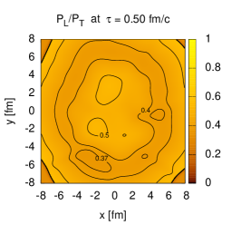
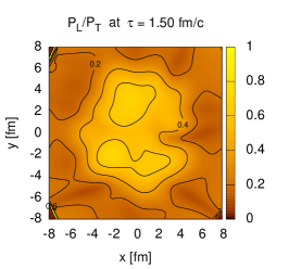
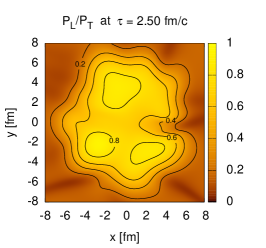
Figure 1: (Color online) Evolution of the pressure anisotropy in a (2+1)-dimensional boost-invariant system subject to a Monte-Carlo Glauber initial condition.

3 Results and Outlook

Having obtained Eqs. (16) and (17) one can solve them to find the spatio-temporal evolution of the energy momentum tensor of an anisotropic system. By construction the transverse and longitudinal pressures obtained in the evolution are guaranteed to be positive. This should be contrasted to solutions to second order viscous hydrodynamics which can result in negative pressures at early times and near the edges of the matter Martinez and Strickland (2009, 2010a). In Fig. 1 we plot the ratio of the LRF longitudinal and transverse pressures at three different proper times. For this figure we assumed a non-central $b=7$ fm collision and used a Monte-Carlo sampled Glauber wounded-nucleon profile, a central $b=0$ isotropic temperature of $\Lambda_{0}=T_{0}=0.6$ GeV at $\tau_{0}=0.25$ fm/c, $\xi_{0}=0$, and $4\pi\eta/S=1$.

As can be seen from Fig. 1, even though the system starts out being perfectly isotropic at $\tau_{0}$, after a very short amount of time the system develops a pressure anisotropy on the order of ${\cal P}_{L}/{\cal P}_{T}\sim$ 0.4 – 0.5 that only slowly relaxes back towards isotropy. One should note, importantly, that this figure is generated assuming the best case scenario for isotropization, namely that $4\pi\eta/S=1$. If one chooses larger values of $\eta$, then one finds larger momentum-space anisotropies at all times. However, regardless of the value of $\eta$, when evolved using Eqs. (16) and (17), the pressures (and in particular the longitudinal pressure) remain positive at all times in the entire transverse plane.

In closing I have briefly reviewed the derivation of (2+1)-dimensional anisotropic hydrodynamics. The full detailed derivation of the equations along with the numerical algorithms necessary are contained in Ref. Martinez et al. (2012). The next step in the development of anisotropic hydrodynamics is to relax the assumption of azimuthal symmetry of the LRF one-particle distribution function in momentum-space. This represents work in progress.

References

- Huovinen et al. (2001) P. Huovinen, P. F. Kolb, U. W. Heinz, P. V. Ruuskanen, and S. A. Voloshin, Phys. Lett. B503, 58–64 (2001), hep-ph/0101136.
- Hirano and Tsuda (2002) T. Hirano, and K. Tsuda, Phys. Rev. C66, 054905 (2002), nucl-th/0205043.
- Israel and Stewart (1979) W. Israel, and J. M. Stewart, Ann. Phys. 118, 341–372 (1979).
- Muronga (2007) A. Muronga, Phys. Rev. C76, 014910 (2007), nucl-th/0611091.
- Luzum and Romatschke (2008) M. Luzum, and P. Romatschke, Phys. Rev. C78, 034915 (2008), 0804.4015.
- Dusling and Teaney (2008) K. Dusling, and D. Teaney, Phys. Rev. C77, 034905 (2008), 0710.5932.
- Peschanski and Saridakis (2009) R. Peschanski, and E. N. Saridakis, Phys.Rev. C80, 024907 (2009), 0906.0941.
- Shen et al. (2011) C. Shen, U. Heinz, P. Huovinen, and H. Song, Phys.Rev. C84, 044903 (2011), 1105.3226.
- Ryblewski and Florkowski (2012) R. Ryblewski, and W. Florkowski, Phys.Rev. C85, 064901 (2012), 1204.2624.
- Martinez and Strickland (2009) M. Martinez, and M. Strickland, Phys. Rev. C79, 044903 (2009), 0902.3834.
- Florkowski and Ryblewski (2011) W. Florkowski, and R. Ryblewski, Phys.Rev. C83, 034907 (2011), %****␣307_Strickland.bbl␣Line␣50␣****1007.0130.
- Martinez and Strickland (2010a) M. Martinez, and M. Strickland, Nucl. Phys. A848, 183–197 (2010a), 1007.0889.
- Ryblewski and Florkowski (2011a) R. Ryblewski, and W. Florkowski, J.Phys.G G38, 015104 (2011a), 1007.4662.
- Martinez and Strickland (2011) M. Martinez, and M. Strickland, Nucl.Phys. A856, 68–87 (2011), 1011.3056.
- Ryblewski and Florkowski (2011b) R. Ryblewski, and W. Florkowski, Eur.Phys.J. C71, 1761 (2011b), 1103.1260.
- Martinez et al. (2012) M. Martinez, R. Ryblewski, and M. Strickland, Phys.Rev. C85, 064913 (2012), 1204.1473.
- Romatschke and Strickland (2003) P. Romatschke, and M. Strickland, Phys. Rev. D68, 036004 (2003).
- Martinez and Strickland (2010b) M. Martinez, and M. Strickland, Phys. Rev. C81, 024906 (2010b).