Magnetic moment of the Roper resonance

Abstract

The magnetic moment of the Roper resonance is calculated in the framework of a low-energy effective field theory of the strong interactions. A systematic power-counting procedure is implemented by applying the complex-mass scheme.

I Introduction

Chiral perturbation theory Weinberg:1979kz ; Gasser:1983yg provides a successful description of the Goldstone boson sector of QCD (see, e.g., Ref. Scherer:2009bt for a recent review). A straightforward power counting, i.e. correspondence between the loop expansion and the chiral expansion in terms of momenta and quark masses at a fixed ratio Gasser:1983yg , is obtained by using dimensional regularization in combination with the modified minimal subtraction scheme. Therefore, a systematic and controllable improvement is possible in perturbative calculations of physical quantities at low energies. The construction of a consistent power counting in effective field theories with heavy degrees of freedom turns out to be a more complex problem. For example, power counting is violated in baryon chiral perturbation theory if dimensional regularization and the minimal subtraction scheme are applied Gasser:1987rb . The problem has been handled by employing the heavy-baryon approach Jenkins:1990jv and, alternatively, by choosing a suitable renormalization scheme Tang:1996ca ; Becher:1999he ; Gegelia:1999gf ; Fuchs:2003qc . Using the mass difference between the nucleon and the $\Delta(1232)$ resonance as an additional expansion parameter, the $\Delta$ resonance can also be consistently included in the framework of effective field theory Hemmert:1997ye ; Pascalutsa:2002pi ; Bernard:2003xf ; Pascalutsa:2006up ; Hacker:2005fh . On the other hand, the inclusion of heavier baryon resonances such as the Roper resonance requires a non-trivial generalization. In this case the problem of power counting can be solved by using the complex-mass scheme (CMS) Stuart:1990 ; Denner:1999gp ; Denner:2006ic ; Actis:2006rc ; Actis:2008uh which can be understood as an extension of the on-mass-shell renormalization scheme to unstable particles. In previous papers we have calculated the pole masses and the widths of the $\rho$ meson and the Roper resonance Djukanovic:2009zn ; Djukanovic:2009gt . In the current paper we consider the magnetic moment of the Roper up to ${\cal O}(q^{3})$. While the extraction of these quantities from experimental measurements at present seems to be unfeasible, our expression for the magnetic moment may be used in the context of lattice QCD. Effective field theories predict the quark-mass dependence of physical observables and can be used to extrapolate simulations in the framework of lattice QCD performed at unphysically large masses of the light quarks. In return, lattice QCD provides a way to determine the low-energy constants from the underlying theory.

II Effective Lagrangian

In this section we specify the effective Lagrangian relevant for the subsequent calculation of the electromagnetic vertex of the Roper at ${\cal O}(q^{3})$. We include the pion, the nucleon, the Roper, and the $\Delta$ as explicit degrees of freedom. The effects of other degrees of freedom are buried in low-energy coupling constants. We write the effective Lagrangian as

$$\mathcal{L}=\mathcal{L}_{0}+{\cal L}_{\pi}+\mathcal{L}_{R}+\mathcal{L}_{NR}+\mathcal{L}_{\Delta R}\,,$$ (1)

where $\mathcal{L}_{0}$ is given by

$$\mathcal{L}_{0} = \bar{N}\,(iD/\hskip 1.00006pt-m_{N0})N+\bar{R}(iD/\hskip 1.00006pt-m_{R0})R$$ (2)

$$-\bar{\Psi}_{\mu}\xi^{\frac{3}{2}}\biggl{[}(i{D/\hskip 1.00006pt}-m_{\Delta 0})\,g^{\mu\nu}-i\,(\gamma^{\mu}D^{\nu}+\gamma^{\nu}D^{\mu})+i\,\gamma^{\mu}{D/\hskip 3.00003pt}\gamma^{\nu}+m_{\Delta 0}\,\gamma^{\mu}\gamma^{\nu}\biggr{]}\xi^{\frac{3}{2}}\Psi_{\nu}.$$

Here, $N$ and $R$ denote nucleon and Roper isospin doublets with bare masses $m_{N0}$ and $m_{R0}$, respectively. $\Psi_{\nu}$ represents the vector-spinor isovector-isospinor Rarita-Schwinger field of the $\Delta$ resonance Rarita:1941mf with bare mass $m_{\Delta 0}$, $\xi^{\frac{3}{2}}$ is the isospin-$3/2$ projector (see Ref. Hacker:2005fh for more details). The covariant derivatives are defined as follows:

$$D_{\mu}H = \left(\partial_{\mu}+\Gamma_{\mu}-i\,v_{\mu}^{(s)}\right)H\,,$$

$$\left(D_{\mu}\Psi\right)_{\nu,i} = \partial_{\mu}\Psi_{\nu,i}-2\,i\,\epsilon_{ijk}\Gamma_{\mu,k}\Psi_{\nu,j}+\Gamma_{\mu}\Psi_{\nu,i}-i\,v_{\mu}^{(s)}\Psi_{\nu,i}\,,$$

$$\Gamma_{\mu} = \frac{1}{2}\,\left[u^{\dagger}\partial_{\mu}u+u\partial_{\mu}u^{\dagger}-i\,\left(u^{\dagger}v_{\mu}u+uv_{\mu}u^{\dagger}\right)\right]=\tau_{k}\Gamma_{\mu,k},$$ (3)

where $H$ stands either for the nucleon or the Roper. The pion fields are contained in the unimodular, unitary, $(2\times 2)$ matrix $U$ and $u=\sqrt{U}$. The external electromagnetic four-vector potential ${\cal A}_{\mu}$ enters into $v_{\mu}=-e\,\frac{\tau_{3}}{2}\,{\cal A}_{\mu}$ and $v_{\mu}^{(s)}=-\frac{e}{2}\,{\cal A}_{\mu}$ ($e^{2}/(4\pi)\approx 1/137,e>0$).

The lowest-order Goldstone-boson Lagrangian including the quark-mass term and the interaction with the external electromagnetic four-vector potential ${\cal A}_{\mu}$ reads

$${\cal L}_{\pi}^{(2)}=\frac{F^{2}}{4}\mbox{Tr}\left(\partial_{\mu}U\partial^{\mu}U^{\dagger}\right)+\frac{F^{2}M^{2}}{4}\mbox{Tr}\left(U^{\dagger}+U\right)+i\,\frac{F^{2}}{2}\mbox{Tr}\left[\left(\partial_{\mu}UU^{\dagger}+\partial_{\mu}U^{\dagger}U\right)v^{\mu}\right]\,.$$ (4)

$F$ denotes the pion-decay constant in the chiral limit: $F_{\pi}=F[1+{\cal O}(q^{2})]=92.4$ MeV; $M$ is the pion mass at leading order in the quark-mass expansion: $M^{2}=2B\hat{m}$, where $B$ is related to the quark condensate $\langle\bar{q}q\rangle_{0}$ in the chiral limit Gasser:1983yg .

The interaction terms $\mathcal{L}_{R}$, $\mathcal{L}_{NR}$, and $\mathcal{L}_{\Delta R}$ are constructed in analogy to Ref. Borasoy:2006fk . The leading-order (${\cal O}(q)$) pion-Roper coupling is given by

$${\cal L}_{R}^{(1)}=\frac{g_{R}}{2}\,\bar{R}\gamma^{\mu}\gamma_{5}u_{\mu}R\,,$$ (5)

where $g_{R}$ is an unknown coupling constant and

$$u_{\mu}=i\left[u^{\dagger}\partial_{\mu}u-u\partial_{\mu}u^{\dagger}-i\,\left(u^{\dagger}v_{\mu}u-uv_{\mu}u^{\dagger}\right)\right].$$ (6)

The second- and third-order Roper Lagrangians relevant for our calculation read

$${\cal L}_{R}^{(2)} = \bar{R}\left[\frac{c_{6}^{*}}{2}\,f^{+}_{\mu\nu}+\frac{c_{7}^{*}}{2}\,v^{(s)}_{\mu\nu}\right]\,\sigma^{\mu\nu}R+\cdots\,,$$

$${\cal L}_{R}^{(3)} = \frac{i}{2}\,d_{6}^{*}\bar{R}\left[D^{\mu},f^{+}_{\mu\nu}\right]\,D^{\nu}R+{\rm H.c.}+2\,i\,d_{7}^{*}\bar{R}\left(\partial^{\mu}v^{(s)}_{\mu\nu}\right)\,D^{\nu}R+{\rm H.c.}+\cdots\,,$$ (7)

where

$$v_{\mu\nu}^{(s)} = \partial_{\mu}v^{(s)}_{\nu}-\partial_{\nu}v^{(s)}_{\mu}\,,$$

$$f_{\mu\nu}^{+} = uf_{\mu\nu}u^{\dagger}+u^{\dagger}f_{\mu\nu}u\,,$$

$$f_{\mu\nu} = \partial_{\mu}v_{\nu}-\partial_{\nu}v_{\mu}-i[v_{\mu},v_{\nu}],$$ (8)

and $c_{6}^{*}$, $c_{7}^{*}$, $d_{6}^{*}$, and $d_{7}^{*}$ are unknown coupling constants. The ellipsis denote those terms of the most general second- and third-order Roper Lagrangians which do not contribute to the electromagnetic vertex of the Roper at ${\cal O}(q^{3})$ and H.c. refers to the Hermitian conjugate. The leading-order interaction between the nucleon and the Roper is given by

$${\cal L}_{NR}^{(1)}=\frac{g_{NR}}{2}\,\bar{R}\gamma^{\mu}\gamma_{5}u_{\mu}N+{\rm H.c.}\,$$ (9)

with an unknown coupling constant $g_{NR}$. Finally, the leading-order interaction between the $\Delta$ and the Roper reads

$${\cal L}_{\Delta R}^{(1)}=-g_{\Delta R}\,\bar{\Psi}_{\mu}\,\xi^{\frac{3}{2}}\,(g^{\mu\nu}+\tilde{z}\,\gamma^{\mu}\gamma^{\nu})\,u_{\nu}\,R+{\rm H.c.}\,,$$ (10)

where $g_{\Delta R}$ is a coupling constant and we take the ”off-mass-shell parameter” $\tilde{z}=-1$. Note that at ${\cal O}(q^{3})$ the $N\Delta$ Lagrangian does not contribute.

III Perturbation theory, renormalization, and power counting

The CMS Stuart:1990 ; Denner:1999gp ; Denner:2006ic ; Actis:2006rc ; Actis:2008uh originates from the Standard Model where it was developed to derive properties of $W$, $Z_{0}$, and Higgs bosons obtained from resonant processes. What makes the situation somewhat different in the case of the strong interactions is the fact that hadrons, including resonances, are thought to be composite objects made of quarks and gluons. The characteristic properties of hadron resonances eventually have to be described by QCD. Within the present effective-field-theory approach, to a given resonance we assign an explicit field with corresponding spin, isospin, and parity content. Furthermore, for a generic resonance $R$, we introduce a complex renormalized mass $z_{\chi}$ defined as the location of the corresponding complex pole position in the chiral limit, $z_{\chi}=m_{R\chi}-i\Gamma_{R\chi}/2$. We assume $\Gamma_{R\chi}$ to be small in comparison to both $m_{R\chi}$ and the scale of spontaneous chiral symmetry breaking, $\Lambda_{\chi}=4\pi F$. Corrections to the complex pole position due to the finite quark masses are treated perturbatively. Our perturbative approach to EFT is based on the path integral formalism. In this framework the physical quantities are obtained from Green’s functions represented by functional integrals. The integration over classical fields corresponding to particles is performed in the standard way, i.e., the Gaussian part is treated non-perturbatively and the rest perturbatively. In particular, the functional integral is performed for both stable and unstable degrees of freedom. For stable particles the path integral formalism is equivalent to the operator formalism based on the Dirac interaction representation. Unfortunately, it is not obvious how to apply this representation to field operators for unstable particles, because, strictly speaking, there is no free Hamiltonian for unstable particles. Therefore, we stick to the functional integral where one can perform the integration independently of the nature of the field.

In the following, we apply the CMS to have a consistent power counting also applicable to loop diagrams. This renormalization scheme is realized by splitting the bare parameters (and fields) of the Lagrangian into, in general, complex renormalized parameters and counter terms. We choose the renormalized masses as the poles of the dressed propagators in the chiral limit:

$$m_{R0} = z_{\chi}+\delta z_{\chi}\,,$$

$$m_{N0} = m_{\chi}+\delta m\,,$$

$$m_{\Delta 0} = z_{\Delta\chi}+\delta z_{\Delta\chi}\,,$$ (11)

where $z_{\chi}$ is the complex pole of the Roper propagator in the chiral limit, $m_{\chi}$ is the mass of the nucleon in the chiral limit, and $z_{\Delta\chi}$ is the complex pole of the $\Delta$ propagator in the chiral limit. We include the renormalized parameters $z_{\chi}$, $m$, and $z_{\Delta\chi}$ in the propagators and treat the counter terms perturbatively. The renormalized couplings $c_{6}^{*}$ and $c_{7}^{*}$ of ${\cal L}_{R}^{(2)}$ are chosen such that the corresponding counter terms exactly cancel the power-counting-violating parts of the loop diagrams.

While the starting point is a Hermitian Lagrangian in terms of bare parameters and fields, the CMS involves complex parameters in the basic Lagrangian and complex counter terms. Although the application of the CMS seems to violate unitarity, the bare Lagrangian is unchanged and unitarity cannot be violated in the complete theory. On the other hand, it is not obvious that the approximate expressions to the $S$-matrix generated by perturbation theory also satisfy the unitarity condition since the conventional Cutkosky cutting equations Cutkosky:1960sp are not valid in the framework of CMS. However, it is possible to derive generalized cutting rules for loop integrals involving propagators with complex masses to show that unitarity is satisfied perturbatively BGJS . In agreement with Ref. Veltman:1963th , the $S$-matrix connecting stable states only is unitary.

We organize our perturbative calculation by applying the standard power counting of Refs. Weinberg:1991um ; Ecker:1995gg to the renormalized diagrams, i.e., an interaction vertex obtained from an ${\cal O}(q^{n})$ Lagrangian counts as order $q^{n}$, a pion propagator as order $q^{-2}$, a nucleon propagator as order $q^{-1}$, and the integration of a loop as order $q^{4}$. In addition, we assign the order $q^{-1}$ to the $\Delta$ propagator and to the Roper propagator. Within the CMS, such a power counting is respected by the renormalized loop diagrams in the range of energies close to the Roper mass. In practice, we implement this scheme by subtracting the loop diagrams at complex ”on-mass-shell” points in the chiral limit.

When calculating an observable, we do not perform an expansion in powers of the mass differences between the Roper and the nucleon or the Roper and the $\Delta$. Rather we calculate the chiral corrections to the magnetic moment of the Roper as a series in powers of the pion mass which is either divided by large scales, like $4\pi F$ and the heavy masses, or multiplied by coupling constants which contain (inverse powers of) hidden large scales. As the omitted neighboring resonances, like $N(1535)$, couple weakly to the Roper resonance, inverse powers of small scales (mass differences between the Roper and the omitted resonances) which are hidden in low-energy coupling constants of our effective theory are enhanced by inverse powers of small couplings (corresponding to the weak coupling of the Roper resonance to its neighbors) and therefore effectively appear as large scales.

The dressed propagator of the Roper can be written as

$$iS_{R}(p)=\frac{i}{p/\hskip 1.00006pt-z_{\chi}-\Sigma_{R}(p/\hskip 1.00006pt)}\,,$$ (12)

where $-i\Sigma_{R}(p/\hskip 1.00006pt)$ denotes the sum of one-particle-irreducible diagrams contributing to the Roper two-point function. The pole of the dressed propagator $S_{R}$ is obtained by solving the equation

$$z-z_{\chi}-\Sigma_{R}(z)=0\,.$$ (13)

We define the pole mass and the width as the real part and $(-2)$ times the imaginary part of the pole Djukanovic:2007bw , respectively,

$$z=m_{R}-i\,\frac{\Gamma_{R}}{2}\,.$$ (14)

Some of the phenomenological analyses and dynamical models describe the Roper as a double-pole structure (see, e.g., Refs. Arndt:1985vj ; Cutkosky:1990zh ). As the self energy in Eq. (13) is a multi-valued function, one might be tempted to look for several solutions of this equation. Although the numbering of sheets is a matter of convention, it is our understanding that in the standard nomenclature only poles on the second sheet are relevant for the physical amplitude and should be interpreted as resonances. Within our perturbative approach, Eq. (13) has a unique solution on the second sheet. This solution is obtained as a power series in terms of the expansion parameter(s) of the perturbation theory.

Figure 1: One-loop self-energy diagrams of the Roper. Dashed and solid lines refer to the pion and nucleon, respectively, and double-solid lines correspond to the Roper and delta. The numbers in the vertices indicate the chiral order.

Close to the pole the Roper propagator can be parameterized as

$$iS_{R}(p)=\frac{i\,Z_{R}}{p/\hskip 1.00006pt-z}+{\rm n.p.}\,.$$ (15)

The residue $Z_{R}$ (wave function renormalization constant of the Roper) is a complex-valued quantity and n.p. stands for the non-pole part. This is in full agreement with Ref. Gegelia:2009py , where we have shown that physical quantities characterizing unstable particles have to be extracted at pole positions using complex-valued wave function renormalization constants. Up to ${\cal O}(q^{3})$, $Z_{R}$ is obtained by calculating the Roper self-energy diagrams shown in Fig. 1. We do not give its explicit expression here.

Figure 2: Tree diagrams contributing to the elastic electromagnetic form factors of the Roper resonance. Double-solid and wiggly lines correspond to the Roper and external electromagnetic source, respectively. The numbers in the vertices indicate the chiral order.

Figure 3: Loop diagrams contributing to the elastic electromagnetic form factors of the Roper resonance. Dashed, wiggly, and solid lines correspond to pion, nucleon, and external electromagnetic source, respectively; double-solid lines correspond to the Roper and $\Delta$. The numbers in the vertices indicate the chiral order.

IV Magnetic moment

Using Lorentz covariance and the discrete symmetries, the most general electromagnetic vertex of a spin-1/2 field may be parameterized in terms of 12 Dirac structures multiplied by form functions depending on three scalar variables, e.g., $p_{i}^{2}$, $p_{f}^{2}$, and $q^{2}$, where $q=p_{f}-p_{i}$ Bincer:1959tz ; Naus:1987kv ; Koch:2001ii . For charged fields, the Ward-Takahashi Ward:1950xp ; Takahashi:1957xn identity provides certain constraints among the form functions. For a stable particle such as the nucleon, on-shell kinematics corresponds to $p_{i}^{2}=p_{f}^{2}=m^{2}_{N}$, and the form functions reduce to conventional form factors of $q^{2}$, say, Dirac and Pauli form factors $F_{1}$ and $F_{2}$, respectively. For unstable particles such as the Roper resonance, the analogous kinematical point is given by the pole position, i.e., $p_{i}^{2}=p_{f}^{2}=z^{2}$. In Ref. Gegelia:2009py we described a method how to extract from the general vertex only those pieces which survive at the pole. To that end, we introduced ”Dirac spinors” $\bar{w}^{i}$ and $w^{j}$ with complex masses $z$ which essentially correspond to half of the projection operators $\Lambda_{+}=\sum_{j}w^{j}\bar{w}^{j}$ used in Refs. Naus:1987kv ; Koch:2001ii for the initial and final lines. In terms of these ”Dirac spinors,” the renormalized vertex function for $p_{f}^{2}=p_{i}^{2}=z^{2}$ may be written in terms of two form factors,

$$\sqrt{Z_{R}}\,\bar{w}^{i}(p_{f})\Gamma^{\mu}(p_{f},p_{i})w^{j}(p_{i})\sqrt{Z_{R}}=\bar{w}^{i}(p_{f})\left[\,\gamma^{\mu}\,F_{1}(q^{2})+\frac{i\,\sigma^{\mu\nu}\,q_{\nu}}{2\,m_{N}}\,F_{2}(q^{2})\,\right]w^{j}(p_{i})\,,$$ (16)

where $m_{N}$ is the physical mass of the nucleon. Both electromagnetic form factors of the Roper are complex-valued functions even for $q^{2}<0$ because of the resonance character of the Roper. As in the case of an on-shell nucleon, the third form function vanishes at the pole because of current conservation or time-reversal invariance.

To ${\cal O}(q^{3})$, the vertex function $\Gamma^{\mu}(p_{f},p_{i})$ obtains contributions from three tree diagrams (see Fig. 2) and fourteen loop diagrams (see Fig. 3). By multiplying the tree-order contribution with the wave function renormalization constant, one subtracts all power-counting-violating contributions of loop diagrams to the $F_{1}$ form factor. We obtain $F_{1}(0)=(1+\tau_{3})/2$ in agreement with the Ward identity. This means that, as expected, the electric charge of the Roper does not receive any strong corrections. On the other hand, the loop contributions to the magnetic form factor contain power-counting-violating terms. These parts are analytic in the squared pion mass and momenta. They are subtracted from the loop diagrams and absorbed in the renormalization of the couplings $c_{6}^{*}$ and $c_{7}^{*}$.

The anomalous magnetic moment in units of the nuclear magneton is defined as

$$\kappa_{R}=F_{2}(0).$$ (17)

Since both the four-momentum $q^{\mu}$ as well as the polarization vector $\epsilon^{\mu}$ count as ${\mathcal{O}}(q)$ our calculation yields the magnetic moment to ${\mathcal{O}}(q)$. The tree-order result for $\kappa_{R}$ is given by

$$\kappa_{R}^{\rm tree}=2\,m_{N}\left(\frac{c_{7}^{*}}{2}+\tau_{3}\,c_{6}^{*}\right).$$ (18)

In order to show that the subtracted loop contributions satisfy the power counting we divide the diagrams of Fig. 3 into three separate classes. Diagrams potentially violating the power counting are loop diagrams with internal Roper, nucleon, and delta lines which we refer to as classes A, B, and C, respectively. We denote the respective contributions to the magnetic moment by $\kappa^{A,B,C}_{R}$.

At first, we consider the contribution of $\kappa^{A}_{R}$. Dividing the expression by $M$ and taking the limit $M\rightarrow 0$ yields

$$\lim_{M\to 0}\frac{\kappa^{A}_{R}}{M}=-g_{R}^{2}\frac{m_{N}}{8\pi F^{2}}\>\tau_{3}.$$ (19)

Replacing the low-energy constant $g_{R}$ with $g_{A}$, this expression coincides with the non-analytic contribution to the anomalous magnetic moment of the nucleon Gasser:1987rb ; Fuchs:2003ir . Next, we analyze the contributions stemming from $\kappa^{B}_{R}$. For a fixed and finite mass difference $z_{\chi}-m_{\chi}$, the limit $M\rightarrow 0$ is zero

$$\lim_{M\rightarrow 0}\frac{\kappa^{B}_{R}}{M}=0.$$ (20)

If $z_{\chi}-m_{\chi}$ scales as $\alpha M$ the limit $M\rightarrow 0$ is given by

$$\lim_{M\rightarrow 0}\frac{\kappa^{B}_{R}}{M}=g_{NR}^{2}\,\frac{m_{N}}{4\pi^{2}F^{2}}\,g\left(\alpha\right)\,\tau_{3},$$ (21)

with

$$g\left(\alpha\right)=i\pi\left(\sqrt{\alpha^{2}-1}-\alpha\right)+\alpha\ln(2\alpha)-\sqrt{\alpha^{2}-1}\ln(\alpha+\sqrt{\alpha^{2}-1}).$$ (22)

Taking the limit $M\rightarrow 0$ after the limit $z_{\chi}\rightarrow m_{\chi}$ results in

$$\lim_{M\rightarrow 0}\,\left(\lim_{m_{\chi}\rightarrow z_{\chi}}\frac{\kappa^{B}_{R}}{M}\right)=-g_{NR}^{2}\,\frac{m_{N}}{8\pi F^{2}}\tau_{3}.$$ (23)

Similar results are obtained for $\kappa^{C}_{R}$. For fixed and finite mass difference $z_{\chi}-z_{\Delta\chi}$ the limit $M\rightarrow 0$ yields

$$\lim_{M\rightarrow 0}\frac{\kappa^{C}_{R}}{M}=0.$$ (24)

If $z_{\chi}-z_{\Delta\chi}$ scales as $\beta M$ the limit $M\rightarrow 0$ is given by

$$\lim_{M\rightarrow 0}\frac{\kappa^{C}_{R}}{M}=g_{\Delta R}^{2}\,\frac{m_{N}}{9\pi^{2}F^{2}}\,g\left(\beta\right)\,\tau_{3}.$$ (25)

Taking the limit $M\rightarrow 0$ after $z_{\chi}\rightarrow z_{\Delta\chi}$ one finds

$$\lim_{M\rightarrow 0}\,\left(\lim_{m_{\Delta}\rightarrow z_{\chi}}\frac{\kappa^{C}_{R}}{M}\right)=-g_{\Delta R}^{2}\,\frac{m_{N}}{18\pi F^{2}}\,\tau_{3}.$$ (26)

The above analysis shows that the renormalized loop diagrams satisfy the power counting regardless of how the various mass differences are treated.

To estimate the loop contributions to the anomalous magnetic moment of the Roper we substitute PDG $F=0.092\,\,{\rm GeV}$, $M=0.140\,\,{\rm GeV}$, $m_{\chi}=0.940\,\,{\rm GeV}$, $z_{\Delta\chi}=(1.210-0.100\,i/2)\,\,{\rm GeV}$, $z_{\chi}=(1.365-0.190\,i/2)\,\,{\rm GeV}$, $\mu=1\,\,{\rm GeV}$, $g_{R}=1$, $g_{\Delta R}=1$, $g_{NR}=0.45$ Borasoy:2006fk and obtain

$$\kappa_{R}=(0.055+0.090\,i)-(0.223+0.156\,i)\,\tau_{3}.$$ (27)

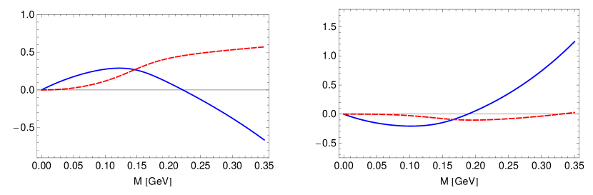
Figure 4: One-loop contributions to the anomalous magnetic moment of the Roper as functions of the pion mass. The left figure corresponds to the neutral and the right to the charged resonances. The solid and dashed lines indicate the real and imaginary parts, respectively.

Figure 4 shows the loop contribution to the anomalous magnetic moment of the Roper as a function of the lowest-order pion mass $M$, where $M^{2}=2B\hat{m}$ GellMann:1968rz .

V Summary

To summarize, we have calculated the magnetic moment of the Roper resonance up to and including order $q^{3}$ using effective-field-theory techniques. To obtain a systematic power counting for energies around the mass of the Roper, we applied the CMS which is a generalization of the on-mass-shell renormalization for unstable particles. Unrenormalized contributions of loop diagrams to the magnetic moment contain power-counting-violating terms. However, these terms are analytic in the squared pion mass and the momenta and can be systematically absorbed in the renormalization of the available low-energy coupling constants. The renormalized loop diagrams satisfy the power counting regardless of how the Roper and nucleon as well as the Roper and delta mass differences are treated.

At next-to-next-to-leading order, ${\mathcal{O}}(q^{3})$, only the isovector anomalous magnetic moment receives a loop contribution. Analogously to the nucleon, the loop contribution to the isoscalar anomalous magnetic moment starts with order ${\mathcal{O}}(q^{4})$. Due to the unstable character of the Roper, the loop contributions to the anomalous magnetic moment feature an imaginary part which is of the same order of magnitude as the corresponding real part.

At present, an extraction of the elastic electromagnetic form factors of the Roper from experimental measurements appears to be unrealistic. However, our expressions for the anomalous magnetic moment may be used in the context of lattice extrapolations. Moreover, lattice QCD provides for an opportunity to determine the five unkown parameters. A fit of our expressions to lattice data at different values for the pion mass results in a complete theoretical prediction of the anomalous magnetic moments of the Roper.

VI appendix

Making use of dimensional regularization with $n$ the number of space-time dimensions, the loop functions are given as Denner:2005nn

$$A_{0}\left(m^{2}\right) = \frac{(2\pi\,\mu)^{4-n}}{i\,\pi^{2}}\,\int\frac{d^{n}k}{k^{2}-m^{2}+i\epsilon}=-32\pi^{2}\lambda\,m^{2}-2\,m^{2}\ln\frac{m}{\mu}\,,$$

$$B_{0}\left(p^{2},m_{1}^{2},m_{2}^{2}\right) = \frac{(2\pi\,\mu)^{4-n}}{i\,\pi^{2}}\,\int\frac{d^{n}k}{\left[k^{2}-m_{1}^{2}+i\epsilon\right]\left[(p+k)^{2}-m_{2}^{2}+i\epsilon\right]}$$

$$= -32\pi^{2}\lambda+2\ln\frac{\mu}{m_{2}}-1-\frac{\omega}{2}\ {}_{2}F_{1}\left(1,2;3;\omega\right)$$

$$-\frac{1}{2}\left(1+\frac{m_{2}^{2}}{m_{1}^{2}(\omega-1)}\right)\,{}_{2}F_{1}\left(1,2;3;1+\frac{m_{2}^{2}}{m_{1}^{2}(\omega-1)}\right)\,,$$

$$\omega = \frac{m_{1}^{2}-m_{2}^{2}+p^{2}+\sqrt{\left(m_{1}^{2}-m_{2}^{2}+p^{2}\right)^{2}-4m_{1}^{2}p^{2}}}{2m_{1}^{2}}\,,$$ (28)

where ${}_{2}F_{1}\left(a,b;c;z\right)$ is the standard hypergeometric function, $\mu$ is the scale parameter of the dimensional regularization and

$$\lambda=\frac{1}{16\,\pi^{2}}\left\{\frac{1}{n-4}-\frac{1}{2}\,\left[\ln(4\pi)+\Gamma^{\prime}(1)+1\right]\right\}\,.$$ (29)

By writing

$$F_{2}(t)=m_{N}[\,G_{1}(t)+\tau_{3}G_{2}(t)],$$ (30)

we obtain the loop contributions as:

$$G_{1}^{\rm loop}(0) = \frac{3g_{R}^{2}}{16F^{2}z_{\chi}\left(M^{2}-4z_{\chi}^{2}\right)\pi^{2}}\Biggl{\{}\left[z_{\chi}^{2}-A_{0}\left(z_{\chi}^{2}\right)-\left(M^{2}-3z_{\chi}^{2}\right)B_{0}\left(z_{\chi}^{2},M^{2},z_{\chi}^{2}\right)\right]M^{2}$$ (31)

$$+\left(M^{2}-2z_{\chi}^{2}\right)A_{0}\left(M^{2}\right)\Biggr{\}}+\frac{3g_{NR}^{2}(m_{\chi}+z_{\chi})^{2}}{64F^{2}m_{\chi}z_{\chi}^{3}\left[(m_{\chi}+z_{\chi})^{2}-M^{2}\right]\pi^{2}}$$

$$\times \Biggl{\{}z_{\chi}A_{0}\left(m_{\chi}^{2}\right)M^{2}+m_{\chi}\left(m_{\chi}(m_{\chi}+z_{\chi})-M^{2}\right)A_{0}\left(M^{2}\right)$$

$$- m_{\chi}\Biggl{[}M^{2}z_{\chi}^{2}+m_{\chi}(m_{\chi}-z_{\chi})\left((m_{\chi}+z_{\chi})^{2}-M^{2}\right)B_{0}\left(z_{\chi}^{2},0,m_{\chi}^{2}\right)$$

$$+ \left(-M^{4}+m_{\chi}(2m_{\chi}+z_{\chi})M^{2}-m_{\chi}(m_{\chi}-z_{\chi})(m_{\chi}+z_{\chi})^{2}\right)B_{0}\left(z_{\chi}^{2},M^{2},m_{\chi}^{2}\right)\Biggr{]}\Biggr{\}}$$

$$+ \frac{g_{\Delta R}^{2}}{864F^{2}z_{\Delta\chi}^{4}z_{\chi}^{3}\pi^{2}}\,\Biggl{\{}-2(z_{\Delta\chi}-z_{\chi})\left(9z_{\Delta\chi}^{4}-14z_{\chi}z_{\Delta\chi}^{3}+8z_{\chi}^{2}z_{\Delta\chi}^{2}+2z_{\chi}^{3}z_{\Delta\chi}+z_{\chi}^{4}\right)$$

$$\times B_{0}\left(z_{\chi}^{2},0,z_{\Delta\chi}^{2}\right)(z_{\Delta\chi}+z_{\chi})^{3}+M^{2}z_{\chi}^{2}\biggl{[}\left(9z_{\Delta\chi}^{2}+4z_{\chi}z_{\Delta\chi}-z_{\chi}^{2}\right)M^{2}$$

$$+ 4z_{\chi}\left(-6z_{\Delta\chi}^{3}-8z_{\chi}z_{\Delta\chi}^{2}+z_{\chi}^{2}z_{\Delta\chi}+4z_{\chi}^{3}\right)\biggr{]}+2\biggl{[}\left(9z_{\Delta\chi}^{2}+4z_{\chi}z_{\Delta\chi}-z_{\chi}^{2}\right)M^{4}$$

$$- (z_{\Delta\chi}+z_{\chi})\left(18z_{\Delta\chi}^{3}-10z_{\chi}z_{\Delta\chi}^{2}+7z_{\chi}^{2}z_{\Delta\chi}-3z_{\chi}^{3}\right)M^{2}$$

$$+ (z_{\Delta\chi}+z_{\chi})^{2}\left(9z_{\Delta\chi}^{4}-14z_{\chi}z_{\Delta\chi}^{3}+8z_{\chi}^{2}z_{\Delta\chi}^{2}+2z_{\chi}^{3}z_{\Delta\chi}+z_{\chi}^{4}\right)\biggr{]}A_{0}\left(M^{2}\right)$$

$$- 2M^{2}\left[\left(9z_{\Delta\chi}^{2}+4z_{\chi}z_{\Delta\chi}-z_{\chi}^{2}\right)M^{2}+2\left(-9z_{\Delta\chi}^{4}-4z_{\chi}z_{\Delta\chi}^{3}+6z_{\chi}^{2}z_{\Delta\chi}^{2}+z_{\chi}^{4}\right)\right]$$

$$\times A_{0}\left(z_{\Delta\chi}^{2}\right)-2\left[M^{2}-(z_{\Delta\chi}+z_{\chi})^{2}\right]\biggl{[}\left(9z_{\Delta\chi}^{2}+4z_{\chi}z_{\Delta\chi}-z_{\chi}^{2}\right)M^{4}$$

$$- 2\biggl{[}9z_{\Delta\chi}^{4}-5z_{\chi}z_{\Delta\chi}^{3}-10z_{\chi}^{2}z_{\Delta\chi}^{2}+z_{\chi}^{3}z_{\Delta\chi}-z_{\chi}^{4}\biggr{]}M^{2}$$

$$+ (z_{\Delta\chi}^{2}-z_{\chi}^{2})\left(9z_{\Delta\chi}^{4}-14z_{\chi}z_{\Delta\chi}^{3}+8z_{\chi}^{2}z_{\Delta\chi}^{2}+2z_{\chi}^{3}z_{\Delta\chi}+z_{\chi}^{4}\right)\biggr{]}B_{0}\left(z_{\chi}^{2},M^{2},z_{\Delta\chi}^{2}\right)\Biggr{\}},$$

$$G_{2}^{\rm loop}(0) = \frac{g_{R}^{2}}{16F^{2}z_{\chi}\left(M^{2}-4z_{\chi}^{2}\right)\pi^{2}}\,\Biggl{\{}-A_{0}\left(z_{\chi}^{2}\right)M^{2}+\left(3M^{2}-10z_{\chi}^{2}\right)A_{0}\left(M^{2}\right)$$ (32)

$$+ z_{\chi}^{2}\left[M^{2}-2\left(M^{2}-4z_{\chi}^{2}\right)B_{0}\left(z_{\chi}^{2},0,z_{\chi}^{2}\right)\right]-\left(3M^{4}-13z_{\chi}^{2}M^{2}+8z_{\chi}^{4}\right)B_{0}\left(z_{\chi}^{2},M^{2},z_{\chi}^{2}\right)\Biggr{\}}$$

$$+ \frac{g_{NR}^{2}(m_{\chi}+z_{\chi})}{64F^{2}m_{\chi}z_{\chi}^{3}\left[(m_{\chi}+z_{\chi})^{2}-M^{2}\right]\pi^{2}}\,\Biggl{\{}(3m_{\chi}-z_{\chi})z_{\chi}A_{0}\left(m_{\chi}^{2}\right)M^{2}+m_{\chi}(m_{\chi}+z_{\chi})$$

$$\times \left(-3M^{2}+3m_{\chi}^{2}+4z_{\chi}^{2}+3m_{\chi}z_{\chi}\right)A_{0}\left(M^{2}\right)+m_{\chi}\Biggl{[}M^{2}(z_{\chi}-3m_{\chi})z_{\chi}^{2}+m_{\chi}\left(3m_{\chi}^{2}+z_{\chi}^{2}\right)$$

$$\times \left[M^{2}-(m_{\chi}+z_{\chi})^{2}\right]B_{0}\left(z_{\chi}^{2},0,m_{\chi}^{2}\right)+(m_{\chi}+z_{\chi})\biggl{[}3M^{4}-\left(6m_{\chi}^{2}+3z_{\chi}m_{\chi}+4z_{\chi}^{2}\right)M^{2}$$

$$+ m_{\chi}(m_{\chi}+z_{\chi})\left(3m_{\chi}^{2}+z_{\chi}^{2}\right)\biggr{]}B_{0}\left(z_{\chi}^{2},M^{2},m_{\chi}^{2}\right)\Biggr{]}\Biggr{\}}$$

$$+ \frac{g_{\Delta R}^{2}}{2592F^{2}z_{\Delta\chi}^{4}z_{\chi}^{3}\pi^{2}}\,\Biggl{\{}z_{\chi}^{2}\Biggl{[}\left(27z_{\Delta\chi}^{2}+20z_{\chi}z_{\Delta\chi}-5z_{\chi}^{2}\right)M^{2}+4z_{\chi}\biggl{(}-18z_{\Delta\chi}^{3}-13z_{\chi}z_{\Delta\chi}^{2}$$

$$+ 5z_{\chi}^{2}z_{\Delta\chi}+20z_{\chi}^{3}\biggr{)}\Biggr{]}M^{2}-2\biggl{[}-54z_{\Delta\chi}^{4}-40z_{\chi}z_{\Delta\chi}^{3}+60z_{\chi}^{2}z_{\Delta\chi}^{2}+10z_{\chi}^{4}$$

$$+ M^{2}\left(27z_{\Delta\chi}^{2}+20z_{\chi}z_{\Delta\chi}-5z_{\chi}^{2}\right)\biggr{]}A_{0}\left(z_{\Delta\chi}^{2}\right)M^{2}+2\biggl{[}5z_{\chi}^{6}+20z_{\Delta\chi}z_{\chi}^{5}$$

$$+ 5\left(3M^{2}-5z_{\Delta\chi}^{2}\right)z_{\chi}^{4}-2z_{\Delta\chi}\left(10M^{2}+53z_{\Delta\chi}^{2}\right)z_{\chi}^{3}-\left(5M^{4}-33z_{\Delta\chi}^{2}M^{2}+55z_{\Delta\chi}^{4}\right)z_{\chi}^{2}$$

$$+ 20z_{\Delta\chi}\left(M^{2}-z_{\Delta\chi}^{2}\right)^{2}z_{\chi}+27\left(z_{\Delta\chi}^{3}-M^{2}z_{\Delta\chi}\right)^{2}\biggr{]}A_{0}\left(M^{2}\right)-2(z_{\Delta\chi}+z_{\chi})^{2}$$

$$\times \left(27z_{\Delta\chi}^{6}-34z_{\chi}z_{\Delta\chi}^{5}-41z_{\chi}^{2}z_{\Delta\chi}^{4}+98z_{\chi}^{3}z_{\Delta\chi}^{3}-17z_{\chi}^{4}z_{\Delta\chi}^{2}-10z_{\chi}^{5}z_{\Delta\chi}-5z_{\chi}^{6}\right)$$

$$\times B_{0}\left(z_{\chi}^{2},0,z_{\Delta\chi}^{2}\right)-2(M-z_{\Delta\chi}-z_{\chi})(M+z_{\Delta\chi}+z_{\chi})\biggl{[}27z_{\Delta\chi}^{6}-34z_{\chi}z_{\Delta\chi}^{5}-41z_{\chi}^{2}z_{\Delta\chi}^{4}$$

$$+ 98z_{\chi}^{3}z_{\Delta\chi}^{3}-17z_{\chi}^{4}z_{\Delta\chi}^{2}-10z_{\chi}^{5}z_{\Delta\chi}-5z_{\chi}^{6}+M^{4}\left(27z_{\Delta\chi}^{2}+20z_{\chi}z_{\Delta\chi}-5z_{\chi}^{2}\right)$$

$$- 2M^{2}\biggl{(}27z_{\Delta\chi}^{4}-7z_{\chi}z_{\Delta\chi}^{3}-50z_{\chi}^{2}z_{\Delta\chi}^{2}+5z_{\chi}^{3}z_{\Delta\chi}-5z_{\chi}^{4}\biggr{)}\biggr{]}B_{0}\left(z_{\chi}^{2},M^{2},z_{\Delta\chi}^{2}\right)\Biggr{\}}.$$

References

• (1) S. Weinberg, Physica A96, 327 (1979).
• (2) J. Gasser and H. Leutwyler, Annals Phys.  158, 142 (1984).
• (3) S. Scherer, Prog. Part. Nucl. Phys.  64, 1 (2010).
• (4) J. Gasser, M. E. Sainio, and A. Švarc, Nucl. Phys.  B307, 779 (1988).
• (5) E. E. Jenkins and A. V. Manohar, Phys. Lett.  B 255, 558 (1991).
• (6) H. B. Tang, arXiv:hep-ph/9607436.
• (7) T. Becher and H. Leutwyler, Eur. Phys. J.  C 9, 643 (1999).
• (8) J. Gegelia and G. Japaridze, Phys. Rev.  D 60, 114038 (1999).
• (9) T. Fuchs, J. Gegelia, G. Japaridze, and S. Scherer, Phys. Rev.  D 68, 056005 (2003).
• (10) T. R. Hemmert, B. R. Holstein, and J. Kambor, J. Phys. G 24, 1831 (1998).
• (11) V. Pascalutsa and D. R. Phillips, Phys. Rev.  C 67, 055202 (2003).
• (12) V. Bernard, T. R. Hemmert, and U.-G. Meißner, Phys. Lett.  B 565, 137 (2003).
• (13) V. Pascalutsa, M. Vanderhaeghen, and S. N. Yang, Phys. Rept.  437, 125 (2007).
• (14) C. Hacker, N. Wies, J. Gegelia, and S. Scherer, Phys. Rev.  C 72, 055203 (2005).
• (15) R. G. Stuart, in ${\rm Z}^{0}$ Physics, ed. J. Tran Thanh Van (Editions Frontieres, Gif-sur-Yvette, 1990), p. 41.
• (16) A. Denner, S. Dittmaier, M. Roth, and D. Wackeroth, Nucl. Phys.  B560, 33 (1999).
• (17) A. Denner and S. Dittmaier, Nucl. Phys. Proc. Suppl.  160, 22 (2006).
• (18) S. Actis and G. Passarino, Nucl. Phys. B777, 100 (2007).
• (19) S. Actis, G. Passarino, C. Sturm, and S. Uccirati, Phys. Lett. B 669, 62 (2008).
• (20) D. Djukanovic, J. Gegelia, A. Keller, and S. Scherer, Phys. Lett.  B 680, 235 (2009).
• (21) D. Djukanovic, J. Gegelia, and S. Scherer, Phys. Lett.  B 690, 123 (2010).
• (22) W. Rarita and J. S. Schwinger, Phys. Rev.  60, 61 (1941).
• (23) B. Borasoy, P. C. Bruns, U.-G. Meißner, and R. Lewis, Phys. Lett.  B 641, 294 (2006).
• (24) R. E. Cutkosky, J. Math. Phys.  1, 429 (1960).
• (25) T. Bauer, J. Gegelia, G. Japaridze, and S. Scherer, in preparation.
• (26) M. J. G. Veltman, Physica 29, 186 (1963).
• (27) S. Weinberg, Nucl. Phys.  B 363, 3 (1991).
• (28) G. Ecker, Prog. Part. Nucl. Phys.  35, 1 (1995).
• (29) D. Djukanovic, J. Gegelia, and S. Scherer, Phys. Rev.  D 76, 037501 (2007).
• (30) J. Gegelia and S. Scherer, Eur. Phys. J.  A 44, 425 (2010).
• (31) R. A. Arndt, J. M. Ford and L. D. Roper, Phys. Rev.  D 32, 1085 (1985).
• (32) R. E. Cutkosky and S. Wang, Phys. Rev.  D 42, 235 (1990).
• (33) A. M. Bincer, Phys. Rev.  118, 855 (1960).
• (34) H. W. L. Naus and J. H. Koch, Phys. Rev. C 36, 2459 (1987).
• (35) J. H. Koch, V. Pascalutsa, and S. Scherer, Phys. Rev. C 65, 045202 (2002).
• (36) J. C. Ward, Phys. Rev.  78, 182 (1950).
• (37) Y. Takahashi, Nuovo Cim.  6, 371 (1957).
• (38) T. Fuchs, J. Gegelia, and S. Scherer, J. Phys. G 30, 1407 (2004).
• (39) K. Nakamura et al. [ Particle Data Group Collaboration ], J. Phys. G 37, 075021 (2010).
• (40) M. Gell-Mann, R. J. Oakes, B. Renner, Phys. Rev.  175, 2195-2199 (1968).
• (41) R. Mertig, M. Bohm, and A. Denner, Comput. Phys. Commun.  64, 345 (1991).
• (42) A. Denner and S. Dittmaier, Nucl. Phys.  B 734, 62 (2006).