Why, when, and how fast innovations are adopted

Abstract

When the full stock of a new product is quickly sold in a few days or weeks, one has the impression that new technologies develop and conquer the market in a very easy way. This may be true for some new technologies, for example the cell phone, but not for others, like the blue-ray. Novelty, usefulness, advertising, price, and fashion are the driving forces behind the adoption of a new product. But, what are the key factors that lead to adopt a new technology? In this paper we propose and investigate a simple model for the adoption of an innovation which depends mainly on three elements: the appeal of the novelty, the inertia or resistance to adopt it, and the interaction with other agents. Social interactions are taken into account in two ways: by imitation and by differentiation, i.e., some agents will be inclined to adopt an innovation if many people do the same, but other will act in the opposite direction, trying to differentiate from the “herd”. We determine the conditions for a successful implantation of the new technology, by considering the strength of advertising and the effect of social interactions. We find a balance between the advertising and the number of anti-herding agents that may block the adoption of a new product. We also compare the effect of social interactions, when agents take into account the behavior of the whole society or just a part of it. In a nutshell, the present model reproduces qualitatively the available data on adoption of innovation.

1 Introduction

What are the factors that determine the adoption by the society of a new technology? The diffusion of technology is an old and classic problem. The usual approach is the one of Everett Rogers Rogers and, according to him, people in a society are Gaussian distributed over the time they take to attach to the novelty. On the left side of the distribution are the innovators, the very first ones to adopt the new technology —even when it has not proven to be useful or reliable—, followed by the early adopters. At the rightmost part of the distribution are located the “laggards” who accept the innovation reluctantly, only when the rest of the society have already changed to it. The majority of the population fits in the middle of the distribution, between an standard deviation of the mean. Integration of the Gaussian gives the total number of adopters as a function of time. A stylized representation of Rogers’ ideas is represented in Figure 1. Empirical results of the consumers behavior of several technologies all along the 20^th century appeared in several sources, including an article of Brimelow in Forbes Forbes , a New York Times article NYT and several blogs blog1 ; blog2 . All the curves exhibit a qualitative behavior similar to the one proposed by Rogers, with the exception that in some cases fully adoption is not attained.

Figure 1: (color online) Dynamics of the adoption of a new technology, according to Rogers Rogers . The extreme left of the Gaussian curve (full line, in blue) correspond to the innovators, while the extreme right to those who resist to adopt. Integrating this Gaussian curve we obtain the total number of adopters as a function of time that follows an error function (dashed line, in red).

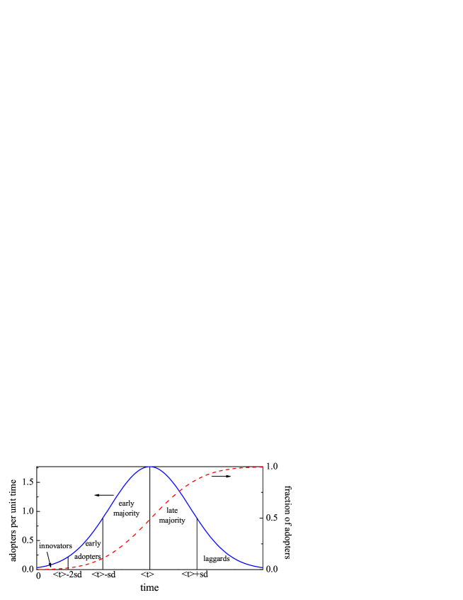
Indeed, some innovations were adopted by practically the totality of the society, like the TV or the refrigerator, while others, like the dishwasher, were adopted by a fraction of the households. Also, the time scales are different for different technologies. Moreover, and as the title of Ref. NYT remarks: innovations are adopted at faster speed today. Examples of this are the following: it was necessary almost forty years (with World War II in between) for the totality of the households to have a refrigerator, thirty years for $90\%$ to have a microwave oven, but only fifteen years for almost $90\%$ to have a cell phone. There is a tendency to faster adoptions in recent times, even if the rapid grow of the B&W TV was omitted in the graphic of Ref. NYT (as discussed in Ref. blog2 ).

The rapid spread of technological novelties is probably a result of massive advertising but also of some kind of fashion and herding effects. As an example, many homes kept the same phone set or refrigerator for many years, while nowadays it is usual to change the cell phone apparatus every one or two years just because of small changes in the functionality upgrade. We should also mention that in some cases the old technology simply disappears and there is no possibility of buying products with the old technology. For instance, electronic injection in automobiles is the standard and cars are no longer made with carburetor. We identify three fundamental external factors in favor of a new technology: utility, advertising pressure, and price. The factors against changing technology are many, but we can mention the facility of keeping a technology which people have a good know-how, a comparable or even better quality (compare the celluloid film with the CCD of the early digital cameras). The lower price is also a relevant factor. However, there is an important factor that have been neglected in classic microeconomics theory masco : the social influence. Collective effects induced by positive (or negative) externalities can be determinant on the decision of buying a good nuttall . Understanding these collective effects is therefore of primary importance vicky ; mirta1 . Social interactions are responsible of the timing in epidemics kup-abram , opinion changes castellano ; us ; galam , outbreaks of social and political unrest galam ; spain , and the willingness to buy a given good mirta2 . Using similar methods other authors studied the fashion market galam2005 or the dynamics of wine purchasing galam2011 . The same kind of social interactions is relevant for the spread of technological innovations. A detailed discussion of social interaction effects may be found in Refs. vicky ; castellano ; galam

Here we describe an artificial society where the external factors in favor of the technological innovation (utility, advertising, and even price) are reduced to a single parameter, that we call “$A$” and assume as objective, i.e. the same for all the agents. This parameter is equivalent in physics to an external field. On the other hand, the resistance to change to a new paradigm, being because of stubbornness, price or familiarity with the old technology, is condensed in the idiosyncratic parameter, $u_{i}$, which is different for each member $i$ of the society. Finally we introduce a social interaction term that may act reinforcing the change of technology, or going contrary to it, if the agent resist to follow the herd. These last agents will be called contrarians, as they will have the tendency to act against the majority. The expression contrarian has been introduced by Galam galam but here we will use it with a slightly different meaning, as it will be discussed below.

The article is organized as follows: In the next section we describe the model, while in Section 3 we present the results, first without the presence of contrarians, and then with a given percentage of them, distinguishing the case where the agents interact with the society as a whole or with a reduced group. Finally, in the last section we discuss the results and present our conclusions, comparing with the data exhibited in Fig. 1.

2 Model

We present a model aim at describing the evolution and dynamics of adoption of a new product, implying a new technology, after it is placed in the market. While consumers can either adopt (buy) or not the novelty, our purpose is to mimic, as good as possible (by comparison with available data) the consumers behavior at large, using the minimal or essential ingredients. The new product can exhibit a completely new technological content, as the personal computer for example, or it may imply an improvement over an existing one, like the new models of smart phones. We assume there is a tendency for the consumer to attach to the old technology for many reasons: to save money, resistance to learn, etc. On the other hand there are advantages in the new product, and the manufacturer tries to emphasize these advantages by means of advertising. Besides, for anyone who has witnessed the teenagers filling the book-stores to grasp the last Harry Potter or Twilight book, or the long lines at the computer stores to buy the new i-Pad, it should be clear that the “imitation” factor has an important role too.

Rogers Rogers calls “innovators” or early adopters the people who gather at the shop entrance the launch day: they are not sure whether the new product is valuable, but they want it because it is new and/or because her/his friend has one. Regarding social interactions, other factors come to play, as in the professional environment, where it is important to share similar technology (smart phones, social networks). Other elements are not less important and act as external pressure, like the widespread use of credit cards or e-forms for bank accounting, airplane or hotel reservations, and tax declarations. The present model tries to include all these factors, plus an additional one: the existence of people acting against fashion, or against the majority. These are the individuals which resist to use cell phones, microwave ovens, or make Internet shopping.

The model consider a set of $N$ interacting agents, each one characterized by two parameters. The first one is the idiosyncratic resistance to change represented by $u_{i}$ ($i$ labels the agent), which is uniformly distributed among the members and assumes values at random in the $[0,1]$ interval. The second parameter, $J_{i}$, is the mean field coupling with the other agents. It can take positive or negative values, the latter case representing contrarian agents. Its effect is to weight the interaction with the people that have already adopted the new technology. Both parameters remain fixed during the adoption process. The marketing force or advertising effect is represented by the parameter $A$ (the same for all members) which acts as an external field.

The dynamics of the system is as follows: each individual $i$ checks the value of the pay-off of adopting the innovation. The pay-off is defined as:

$$P=A-u_{i}+J_{i}n$$ (1)

where $n$ is the fraction of adopters of the new technology ($n=\frac{N_{adop}}{N}$). Agent $i$ adopts the new technology if the pay-off is positive ($P>0$). Otherwise it remains with the old one. We remark that the pay-off of Eq. 1 with $J_{i}>0$ is very similar to the one used in a study of markets with externalities mirta1 . The difference resides in the fact that in Ref. mirta1 the positive quantity is the willingness to buy, that changes from agent to agent, and the negative term is the price that is the same for all agents. Here the positive term (advertising) is constant and the resistance to adoption is negative and idiosyncratic (changes from agent to agent).

The present model, condensed in the pay-off expression Eq.(1), is a mean field model, meaning that every agent “feels” the influence of all the rest. As it was stated previously, we have added a second feature: the presence of a certain percentage of agents with $J_{i}<0$ which act against the innovation, being the opposition stronger the higher the number of adopters. We denominate these agents, following Ref. galam , “contrarians”, even when our definition is not exactly the same of Galam. He defines a contrarian as an agent that acts always against the majority, here, a contrarian agent, when selected in the simulation, interacts with the adopting agents with a negative $J_{i}$. While Eq. 1 for $J_{i}<0$ resembles an anti-ferromagnetic interaction, it is not, because $J_{i}$ does not weigh a pair interaction between two agents, but it weighs the interaction between one agent and the bulk.

Another variant of the model considers groups of influence. In this case, each agent, instead of experiencing the effect of all the others, feels the influence of a subset of them, selected at random from the population.

We also investigate a different distribution of the idiosyncratic resistance to change $u_{i}$, considering a triangular distribution as the simplest approach to the Gaussian distribution proposed in Ref. Rogers .

In the next section we present the results for the basic model and the three variants.

3 Results

A mean field analysis of the basic model (no contrarians, i.e., $J_{i}=J>0$ for all the agents, uniform distribution of $u_{i}$, and no groups of influence) is readily straightforward. We first describe this case where some results can be obtained in an analytical way and verified by the simulations.

3.1 Basic model

Starting with the whole population not having the new technology ($n=0$ in Eq. 1), the fraction of agents for which $u_{i}\leq A$ will shift to the new technology. They will become the new adopters, or the innovators according to Rogers Rogers , those who can be convinced by the sole effect of publicity. How many individuals will adopt the new product as soon as they are aware of it will depend on the force of the campaign measured by $A$. As the values of $u_{i}$ are randomly and uniformly distributed in the $[0,1]$ interval, the number of individuals with values of $u_{i}$ below $A$ is $N_{adop}\approx AN$. Then, after the first time step we have a fraction $n=N_{adop}/N=A$ of new adopters. In the next step (of an arbitrary unit time) those who have $u_{i}\leq(A+Jn)=(A+JA)$ will convert too, i.e. those who had less temptation to try the novelty but will go after seeing that some people already adopted it. If $J=1$, the adopters after the second step will be those with $u_{i}\leq 2A$. Following in this way, the society evolves, at constant pace, into full adoption after a finite number of steps, equal to $A^{-1}$. If $J<1$ however, the iterative process give rise to a geometric series describing the dynamics: $n(t)=A\sum_{i=0}^{t}J^{i}$, with asymptotic value $n(\infty)=A/(1-J)$. Thus, for $J=1$, at any value of $A$, the whole society will adopt the new technology; the intensity of $A$ will just determine the speed of this transformation. For lower values of $J$ there will be a finite fraction of the population adopting the innovation. These results are verified by numerical simulations, as can be seen in Fig. 2. The simulation is performed using a Monte Carlo (MC) method, i.e., choosing one agent at random and applying Eq. 1. If the payoff is positive the agent become an adopter. One MC step corresponds to choosing N agents at random, where N is the size of the system.

Figure 2: (color online) Fraction of new adopters as a function of time (in MC steps) for marketing value $A=0.01$, system size $N=10^{7}$, and for different values of the coupling parameter $J$. The effect of the social interactions is remarkable. It is evident that it is not possible to have full adoption when $J<1$.

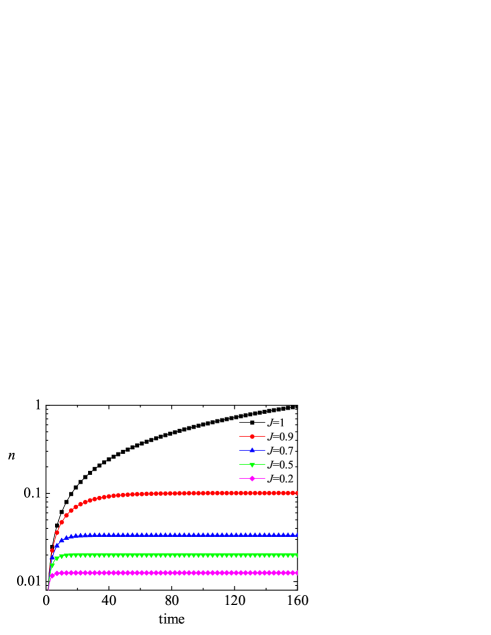
We can see in the figure (Fig. 2) some examples of the temporal evolution of the fraction of new adopters for $N=10^{7}$, different values of the coupling parameter $J$ and a fixed marketing value $A=0.01$. The effect of the social interactions is remarkable. It is evident that it is not possible to have full adoption when $J<1$. On the other hand, in Fig. 3 we show a complementary point of view: considering again $N=10^{7}$ agents, but for a fixed value of the coupling parameter, $J=1$, we show the fraction of adopters as a function of time for different values of the advertising $A$. We can verify that the number of adopters increases linearly with time but the slope is lower than $A$, the analytically predicted value. This is so because when doing the MC simulation in a finite system, the population is not covered exhaustively. As a consequence, agents will change opinion only when “visited” in the MC dynamics. The probability of an agent not to be chosen in a MC step is $(1-1/N)^{N}$, which in the limit of large $N$ is equal to $\exp(-1)$; then the fraction of chosen agents is $1-\exp(-1)=0.632$, so the slope is $0.632A$ (as can be checked in Fig. 3). If the simulations are performed sequentially, picking all the agents at each MC step, the speed of the adoption is very close to $A$ (open symbols in Fig. 3). But even if the evolution is slower in the non-sequential MC dynamics, the final values are not affected by the type of simulation. Therefore, we decided to keep the MC type simulation as we think it better represents the dynamics of a real society.

Figure 3: (color online) Fraction of new adopters as a function of time (in MC steps) for $J=1$, $N=10^{7}$ and different marketing values $A$. Each curve is a single run. Even for a very small advertising ($A=0.001$) full adoption is obtained if $J=1$. Full symbols correspond to pick agents randomly, whereas open symbols correspond to select them sequentially.

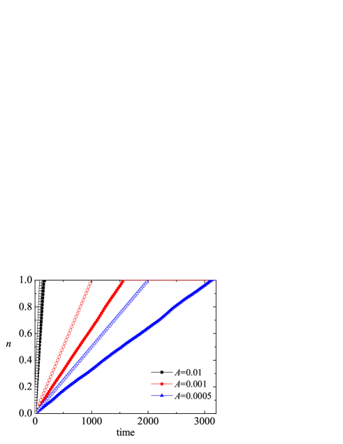
The results for this kind of society are quite simple: if the social interaction $J$ is strong enough, after a time that depends on the intensity of the advertising, the full society will adopt the innovation. On the other hand if the social influence is weak compared with the maximum value of the idiosyncrasy $u_{i}$ of the agents, only a finite fraction, which depends on the values of $J$ and $A$, will adopt the innovation.

3.2 Model with contrarians

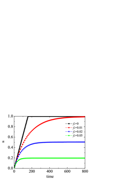
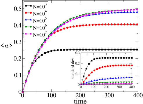
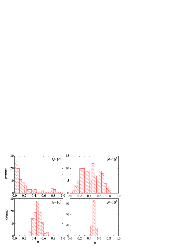
In this section we explore the effect of having a part of the population reacting in opposition to the majority. We call these agents contrarians and they are characterized, in terms of the model, by having a negative $J_{i}$ coupling. All along this section we assume $|J_{i}|=1$ and, as agents do not change their idiosyncrasy in time, the number of contrarians will be constant in time. We define the fraction of contrarians, $f_{c}$, as the portion of the population having $J_{i}=-1$. We have represented in Fig. 4 the fraction of agents adopting the new technology as a function of time for a fixed value of the advertising, $A=0.01$, and four different fractions of contrarians. The size of the system is $N=10^{7}$ agents. In the absence of contrarians we recover the previous result: the entire society adopts the innovation. Yet, a small concentration of contrarians is enough to reduce the fraction of adopters by a significant fraction; for example $f_{c}=0.02$ decreases the fraction of adopters by a half. We must say, however, that these results strongly depend on the size of the samples. On Fig. 5 we represent an average over $100$ samples of the temporal evolution for different system sizes, for the case $A=0.01$, and $f_{c}=0.02$. While in the previous figure (Fig. 4, $N=10^{7}$) the fraction of adopters converge to $50\%$ for $f_{c}=0.02$, we can see that for smaller samples the number of adopters may be bigger, up to $75\%$ for $N=10^{3}$. Also, the fraction of adopters exhibit large fluctuations for small systems at all times, as it can also be observed on Fig. 5. The dispersion goes down with $1/\sqrt{N}$. The finite size effects can also be visualized by performing an statistical study over the final state for the different samples. On Fig. 6 we have represented by histograms the distribution of the asymptotic number of adopters over $100$ samples and four different sizes of the system. We can verify that for smaller systems the distribution is very wide —even Poisson-like for $N=10^{3}$ agents—, but they became narrower as the system size increases. After these considerations, in the following (and as it was in the previous section) we consider a number of agents $N=10^{7}$.

Figure 4: (color online) Fraction of adopters of the new technology as a function of time, for four different values of the fraction of contrarians: $f_{c}=0$, $0.01$, $0.02$ and $0.05$. In all cases, $A=0.01$ and $N=10^{7}$.

Figure 5: (color online) Finite size effects: Average time evolution of the system for different sizes. For each curve, symbols represent averages taken over $100$ runs. Inset: The standard deviation of the averages shown in the main panel. For $N\geqslant 10^{6}$ we can say that the evolution is independent of the size of the sample.

Figure 6: Finite size effects: Histograms of the final number of adopters for $100$ samples and four different system sizes from $10^{3}$ to $10^{6}$, with $A=0.01$ and a fraction of contrarians $f_{c}=0.02$.

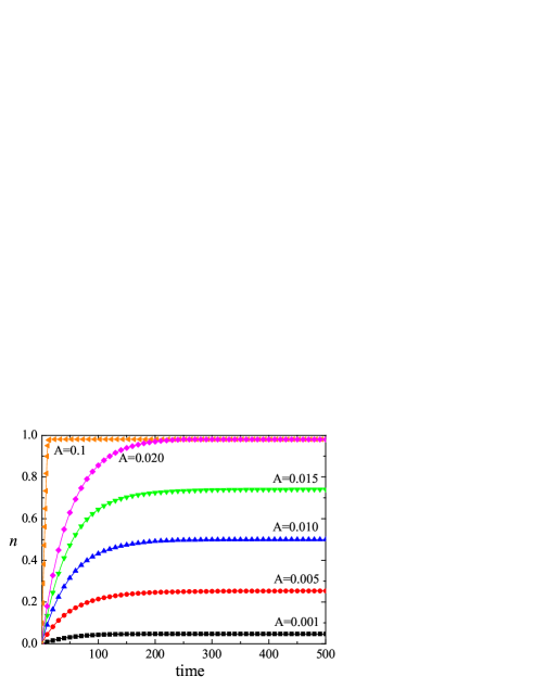
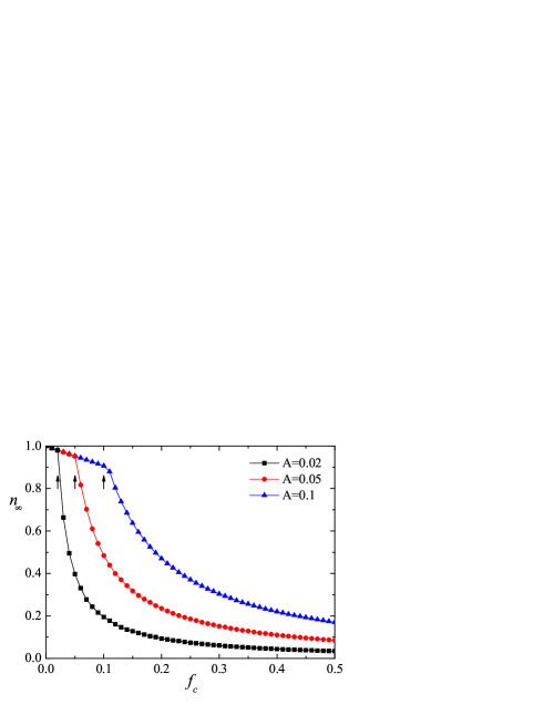
Now we turn to analyze the simultaneous effect of advertising and contrarians. This is represented in Fig. 7 for a fixed percentage of contrarians ($f_{c}=0.02$) and different values of $A$. It is clear from the figure that there is a critical value of advertising to obtain the maximum adoption of the innovation by the society. Due to the presence of contrarians the maximum fraction of adopters is bounded by $1-f_{c}$. The number of adopters increases linearly as the number of contrarians decreases or as the advertising increases, until $f_{c}=A$, when a clear change in the behavior is observed. Fig. 7 shows that when $A\geq f_{c}$ the maximum possible adoption ($1-f_{c}$) is reached. This can be best appreciated by looking at it from another angle: for a fixed advertising value $A$, above the critical value $f_{c}=A$ the number of adopter falls abruptly and in inverse proportion to $f_{c}$, as shown in Fig. 8. Interestingly, a relatively small percentage of contrarians may block the maximum possible adoption of the innovation or force a stronger advertising (i.e. $A\geq f_{c}$) campaign in order to impose the innovation. Therefore, it is evident from Figs. 7 and 8 that the system converges to the maximum adoption only when the advertising is strong enough, $A\geq f_{c}$, and also that the number of adopters grows with time, more and less linearly, up to a saturation point.

Figure 7: (Color online) Effect of the advertising $A$ for a fixed percentage of contrarians $f_{c}=0.02$. Each curve is a single run with $N=10^{7}$.

Figure 8: (Color online) Final proportion of adopters as a function of the fraction of contrarians for three different values of the advertising. Each point represents the final state of a single run with $N=10^{7}$ (lines are just a guide to the eye). Arrows indicate the critical value $f_{c}=A$.

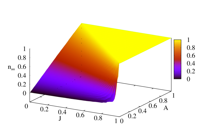
The results of the first two subsections can be summarized in a $3D$ diagram. On Fig. 9 we show the final fraction of adopters on the $z$-axis as a function of the social interaction $J$ on the $x$-axis and of the advertising $A$ on the $y$-axis, for a fixed fraction of contrarians: $f_{c}=0.02$. A sharp but continuous transition as a function of $A$ is observed for high values of $J$, while the transition is smoother and converges to a smaller number of adopters for intermediate values of $J$ and $A$.

Figure 9: (Color online) Final fraction of adopters as a function of $J$ and $A$, for $f_{c}=0.02$

Finally, we would like to emphasize that allowing or not the contrarians to adopt the new technology is mostly irrelevant. In other words, allow them to check their pay-off function (Eq. 1) to take a decision, or keep them in a permanent non-adopter state, yields the same result. This is because the higher the number of adopters $n$, the stronger the negative effect on the payoff of the contrarians, and thus it will be very difficult for a whimsical contrarian to become an adopter, even if her/his resistance $u_{i}$ is low. In effect, our contrarians are much closer to inflexibles than to the contrarians of Galam galam2011b .

3.3 Groups of influence

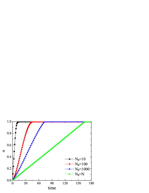
In the preceding section we have implicitly considered that each agent in the society knows exactly what all the other agents have chosen, because we used $n=N_{adop}/N$ (where $N_{adop}$ is the number of adopters of the new technology and $N$ is the total number of agents) as the fraction of adopters to plug into its payoff. However, nobody can have such instant and exact account of how the rest of the society (or country, or city) is reacting to the novelty. Most probably he/she will have an imperfect sense of that through the news, or better from what people around him/her (family, friends, colleagues, etc) are doing. Besides, from the technical point of view, we have seen that the size of the sample is important for the results. Then, we consider in this subsection that people interact with a group much smaller than the whole society, i.e. the number of members of the influence group is $N_{g}<<N$. We calculate the payoff using the same Eq. 1 but now with $n^{\prime}=N_{adop,g}/N_{g}$, where $N_{adop,g}$ is the number of adopters within the group of influence of size $N_{g}$.

While in the real life the groups of influence can vary from person to person, we make a simpler approach here assuming that all the groups of influence have the same size, and that the members of the groups are chosen at random. In other words, at each MC step and for each agent, we choose a set of $N_{g}$ other agents at random from the population and the state of them is used in the payoff. So the size of the groups is fixed and the same for all agents, while the members of them are chosen at random at every time step. Notice that groups are not isolated because any group has overlapping members with another group (in principle it is possible but highly improbable for a group to be isolated). We first analyze the case without contrarians. We have represented on Fig. 10 the time evolution of the number of adopters for similar parameters than in the previous section: $J=1$, $A=0.01$, $N=10^{7}$ and for different sizes of the groups of influence. It can be observed that the system converges to full adoption faster when the size of the groups of influence is smaller. This means that the effect of small groups is more effective to spread the new technology. Comparing this results with the case with zero contrarians, represented in Fig. 4, is clear that the time necessary to converge to complete adoption is much shorter with than without groups of influence. Moreover, we have verified that in the case of groups of influence the determinant factor is the size of the groups and not the size of the whole society. In other words, the evolution of the number of adopters for a fixed size of the group of influence is almost independent of the sample size.

Figure 10: (Color online) Number of adopters for $N=10^{7}$, $A=0.01$, $J=1$, and zero contrarians, with three different sizes of the groups of influence: $N_{g}=10$, $100$ and $1000$. It is worth to note that the convergence to a state of complete adoption is faster the smaller is the group of influence. This means that close contacts are more effective than the “diluted” interaction with all the agents.

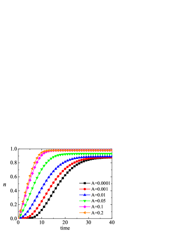
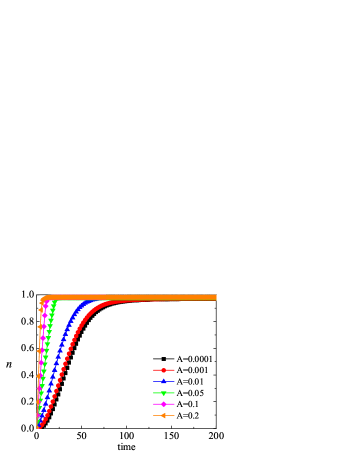
If we include now the contrarians, the results are very rich and in some cases correspond very well to the adoption empirical curves of US consumers, represented in Fig.1. To study in full detail the combined effect of contrarians and groups of influence we have represented different cases in Fig. 11. One evident result is that the number of adopters increases as swiftly as in the case without contrarians. However, and at variance with previous results, even for $A\geq f_{c}$ the system does not arrives at full adoption, i.e. the effect of the contrarians is somehow amplified by the groups of influence: the smaller the group, the bigger the effect. To verify this result, in the left panel of Fig. 11 we have represented the results for a group of influence $N_{g}=10$, while in the right panel we show the results for $N_{g}=100$. When increasing the size of the group of influence, other parameters fixed, the system approaches a behavior closer to the mean field results.

Figure 11: (Color online) Evolution of the number of adopters for $J=1$, $f_{c}=0.02$, and $N=10^{7}$, for different values of the advertising $A$ and for two groups of influence: $N_{g}=10$ (left panel) and $N_{g}=100$ (right panel). Notice that the time scale is different in the two panels, although the final fraction of adopters is, in all the cases, $n=1-f_{c}=0.98$.

In short, the effect of groups of influence is very interesting and induces behaviors that are different from the mean field results, and closer to practical situations. The importance of the effect of interactions in small groups in driven the society to adopt a given opinion or decision has been extensively discussed by Galam galam ; galam2011 and similar results are also reported in ref. Hub when comparing the effect of friends and global opinions when taking a decision to buy or not a product. In any case, it is worth notice that the adoption curves, when groups of influence are included, look more similar to the empirical results quoted in the introduction Rogers ; Forbes ; NYT .

3.4 Triangular Distribution

A possible objection to the preceding results is that we considered a uniform distribution of the idiosyncratic resistance to change $u_{i}$, while the hypothesis of Rogers Rogers is that this distribution is Gaussian (See Fig. 1). We can argue that the results with groups of influence reproduce in a qualitative way the proposed curve of adoption of Rogers, and also the empirical curves Forbes ; NYT , but for the seek of completeness we investigate a different distribution of the idiosyncratic resistance to change. Let us briefly consider a triangular distribution centered in $\langle u\rangle=0.5$, that is a rough but simple approach to the Gaussian distribution.

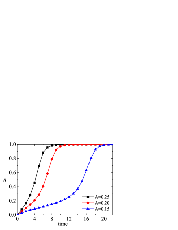
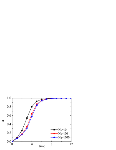
On Fig. 12 we have represented the adoption curves for a triangular distribution of $u_{i}$ and without contrarians. The left panel shows the results for the mean field model (i.e., the model with no groups of influence) and three different values of the advertising $A$. In the right panel, the effect of different sizes for the groups of influence is displayed. It is worth to say that, in order to have the expected behavior, we have to consider higher values of the advertising. This is because the triangular distribution has a smaller number of early adopters when compared with the uniform distribution. We have also verified that with the triangular distribution of $u_{i}$, contrarians have a very weak effect, so results considering contrarians have been omitted.

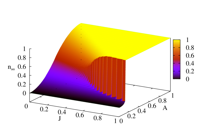
Besides, the inclusion of a non-uniform (triangular) distribution of $u_{i}$ brings a novel result which is showed in Fig. 13. Such figure represents, in $3D$, the asymptotic fraction of adopters, $n$, as a function of $J$ and $A$, exhibiting a clear phase transition as a function of $A$ for values of $J\geq 0.5$. This is in agreement with the phase transition obtained in Ref. mirta1 and it means that the number of adopters can suffer an abrupt and discontinuous change as a function of the advertising.

Figure 12: (Color online) Evolution of the number of adopters for a triangular distribution of idiosyncratic resistance to change and for $J=1$, $N=10^{7}$, and no contrarians. Left panel: different values of the advertising $A$ without groups of influence. Right panel: different sizes of the groups of influence for $A=0.2$.

Figure 13: (Color online) Phase diagram of the final fraction of new adopters $n$ as a function of the coupling parameter $J$ and of the advertising $A$.

4 Discussion and Conclusions

We have presented a model of adoption of a new technology that, in spite of its simplicity, captures the essential features of the behavior of societies: a distribution of an idiosyncratic resistance to change, the power of advertising, the effect of social interactions, and the presence of people who act against the general behavior. The effect of each one of these factors has been investigated separately as well as in combination.

A relatively weak social interaction (either because of a low value of the interaction parameter $J$ or by a low advertising $A$), can impede the adoption of the new technology by the full society. Such can be the case of products with a limited penetration like the dishwasher or the blue-ray player.

Moreover, the inclusion of a small concentration of contrarians in the model is enough to reduce the fraction of adopters by a significant fraction. They may force a stronger advertising campaign in order to impose the innovation.

Regarding again the social interaction, we observed that small groups of influence may be a determinant factor both in the speed of adoption as well as in the percentage of the population adopting the new technology. We have verified that the interaction with small groups instead of with the full society may explain the general behavior of the empirical adoption curves Forbes ; NYT . Also, different speeds of adoption may be obtained by changing the size of the groups of influence, the strength of the advertising, or the percentage of contrarians.

Considering a triangular distribution of the idiosyncratic resistance to change can also result in adoption curves with profiles similar to the empirical results. Besides, in this case it can exists an abrupt transition in the final number of adopters as a function of the advertising. Otherwise, even if a relatively slow growth of adoption may be observed in some cases in Fig 12, the triangular distribution does not provide a wide variety of speeds of adoption. In other words, the triangular distribution seems to be insensitive to the size of the groups of influence.

Our results indicate that, on one side, the acceleration of the adoption velocity is a combined effect of the advertising (Fig. 2) and of the size of the groups of influence (Fig. 11). On the other side, attaining or not full adoption depends on both, the strength of the social interaction and the fraction of contrarians.

Finally we want to emphasize that the present model represents a mean field approach, regarding the interaction with the bulk (or a random subgroup), without taking into account any possible network topology. Remarkably, in spite of that, the model is able to reproduce the essential features of the adoption of a new technology. However, we realize that the effect of distributing the agents on a network could have some relevant effect in the dynamics of technology adoption, and such is the subject of a work already in progress.

5 Acknowledgments

JRI thanks the kind hospitality of the Statistical and Interdisciplinary Physics Group of Instituto Balseiro in S.C. de Bariloche, Argentina and acknowledges the financial support of a “Dr. César Milstein” grant from the program Raíces of the Ministerio de Ciencia Tecnología e Innovación Productiva of Argentina.

The authors acknowledge support from Brazilian agency CNPq and from projects CNPq/Prosul 49044/2007 and FAPERGS-Pronex.

References

- (1) E. M. Rogers. Diffusion of Innovations. 5th edition, Free Press, 2003.
- (2) P. Brimelow. The silent boom. Forbes, http://www.forbes.com/forbes/1997/0707/6001170a.html, 1997.
- (3) Michael Cox and Richard Alm. You are what you spend. New York Times, February 10th 2008.
- (4) A. Thierer. On Measuring Technology Diffusion Rates. http://techliberation.com/2009/05/28/on-measuring-technology-diffusion-rates/, 2009.
- (5) D. Algoso. What does complexity mean? What do we do about it?. Find What Works. http://findwhatworks.wordpress.com/tag/technology-adoption/, 2010.
- (6) A. Mas-Collel, M.D. Whiston, and J.R. Green. Microeconomic Theory. Oxford University Press, New York, 1995.
- (7) W.J. Nuttall, T. Zhang, D.J. Hamilton, and F.A. Roques. Sociophysics Simulations of Technology Adoption and Consumer Behavior. Second International Symposium on Engineering Systems MIT, Cambridge, Massachusetts, June 15-17, 2009. (http://ima.ac.uk/papers/zhang2009.pdf)
- (8) V. Semeshenko. Interacting learning agents: Models, Simulations and Experiments. VDM Verlag. ISBN-13: 978-3639190946, 2009.
- (9) Jean-Pierre Nadal, Denis Phan, Mirta B. Gordon, Jean Vannimenus. Multiple equilibria in a monopoly market with heterogeneous agents and externalities. Quantitative Finance vol 5, No6, 557-568, 2005.
- (10) M. Kuperman and G. Abramson. Small world effect in an epidemiological model. Phys Rev Lett. 86, 2909, 2001.
- (11) C. Castellano, S. Fortunato and V. Loreto. Statistical physics of social dynamics. Rev. Mod. Phys. 81, 591646, 2009.
- (12) M. F. Laguna, S. R. Gusman, G. Abramson, S. Gonçalves, and J. R. Iglesias. Dynamics of opinion in hierarchical organizations. Physica A 351, 580-592, 2005.
- (13) S. Galam. Sociophysics: a review of Galam models. International Journal of Modern Physics C 19, No3, 409440, 2008.
- (14) http://en.wikipedia.org/wiki/2011_Spanish_protests
- (15) Mirta B. Gordon, Jean-Pierre Nadal, Denis Phanc, and Jean Vannimenus. Sellers dilemma due to social interactions between customers. Physica A 356, 628640, 2005.
- (16) S. Galam and A. Vignes. Fashion, novelty and optimality: an application from Physics. Physica A 351, 605-619, 2005.
- (17) T. Bouzdine-Chameeva and S. Galam. Word-of-mouth versus Experts and Reputation in the Individual Dynamics of Wine Purchasing. Advances in Complex Systems 14, 871885, 2011.
- (18) S. Galam. Collective Beliefs versus Individual Inflexibility: The Unavoidable Biases of a Public Debate. Physica A 390, 30363054, 2011.
- (19) Z. Abbassi, Christina Aperjis and Bernardo A. Huberman. Swayed by Friends or by the Crowd?. arXiv:1111.0307v2, 2011.