Shear-Driven Circulation Patterns in Lipid Membrane Vesicles

Abstract

Recent experiments have shown that when a near-hemispherical lipid vesicle attached to a solid surface is subjected to a simple shear flow it exhibits a pattern of membrane circulation much like a dipole vortex. This is in marked contrast to the toroidal circulation that would occur in the related problem of a drop of immiscible fluid attached to a surface and subjected to shear. This profound difference in flow patterns arises from the lateral incompressibility of the membrane, which restricts the observable flows to those in which the velocity field in the membrane is two-dimensionally divergence free. Here we study these circulation patterns within the simplest model of membrane fluid dynamics. A systematic expansion of the flow field based on Papkovich–Neuber potentials is developed for general viscosity ratios between the membrane and the surrounding fluids. Comparison with experimental results [C. Vézy, G. Massiera, and A. Viallat, Soft Matter 3, 844 (2007)] is made, and it is shown how such studies could allow measurements of the membrane viscosity. Issues of symmetry-breaking and pattern selection are discussed.

1 Introduction

One of the defining features of plant cells is the vacuole, an organelle filled with water that acts as a nutrient storehouse for the cytoplasm. The vacuole is contained within the vacuolar membrane, a lipid bilayer structure known also as the tonoplast. It is a nearly ubiquitous feature of plants that the cytoplasm, the thin fluid layer surrounding the vacuolar membrane, is in constant motion through the phenomenon of cytoplasmic streaming (Verchot-Lubicz & Goldstein, 2010) in which motor proteins move along filaments and entrain fluid. Dating back to important work by Pickard (1972) it has been suggested that the shear created in the cytoplasm is fully transmitted through the tonoplast into the vacuolar fluid, a conjecture supported indirectly by recent whole-cell measurements of the streaming velocity profile in large plant cells (van de Meent et al., 2010).

In considering the dynamics of shear transmission across the tonoplast, ideas may be drawn from the large body of work on the response to flow of lipid vesicles. These are closed bilayer membrane structures enclosing fluid, whose membrane is generally in the ‘fluid’ phase with zero shear modulus. These studies constitute a highly active area of research complementing the well-established understanding of membranes in thermal equilibrium (Seifert, 1997). The first insights into vesicle motion under flow were made when Keller & Skalak (1982) described prototypical ‘tank-treading’ and ‘tumbling’ behaviour. Further developments were quickly made in the context of red blood cell dynamics; Barthes-Biesel & Sgaier (1985) used a visco-elastic membrane model to understand the observed tank-treading behaviour, and Feng et al. (1989) provided detailed insights into the precise structure of the area-preserving membrane flow patterns. However, it is more recently that advances have been made in understanding the full three-dimensional behaviour of nearly-spherical vesicles (Seifert, 1999), revealing a rich phase space of both stable (Misbah, 2006; Lebedev et al., 2007; Deschamps et al., 2009; Zhao & Shaqfeh, 2011) and unstable (Kantsler et al., 2007) behaviours.

Less well-studied has been the hydrodynamics of vesicles when constrained to lie stuck to a surface. Such problems arise as the natural extension of considering the flow of these objects near to walls, since adhesion can occur upon the vesicle coming into contact with the surface (Abkarian & Viallat, 2008). Indeed, the elementary problem of an immiscible fluid droplet in contact with a no-slip plane immersed in a bulk flow, absent the interfacial membrane of a vesicle, is one that has attracted detailed study. Dussan V. (1987) performed a comprehensive theoretical study of the behaviour of shallow droplets in such situations, deriving a flow pattern whereby the droplet flows with the applied shear on the surface and recirculates back underneath inside. Sugiyama & Sbragaglia (2008) considered a perfectly hemispherical droplet with similar conclusions. The presence of an interfacial membrane disallows such flows, since they are not area-conserving and the membrane is unable to flow back through the vesicle, and so a qualitatively different flow pattern is guaranteed simply by the inclusion of the membrane.

Lorz et al. (2000) studied the weak adhesion of vesicles and observed a tank-treading type behaviour of the membrane under shear flow, with symmetric recirculating regions on either side of the vesicle midline. To further quantify the membrane hydrodynamics, Vézy et al. (2007) studied adhered vesicles in shear flow with varying contact areas, and observed the same symmetric doubly-recirculating pattern of motion of the membrane in all cases. These experiments have yet to be complemented by any theoretical modelling and calculation of the expected membrane and bulk flow patterns in such geometries. Therefore, as a first step towards understanding these observations we formulate here a simplified theory for a vesicle adhered to a flat substrate subjected to shear flow. The vesicle is assumed to be an axisymmetric spherical cap, and the membrane to be an impermeable, two-dimensional, incompressible Newtonian fluid, where we approximate the bilayer structure of the membrane as a single layer by assuming zero inter-layer slip. On the phenomenological length scales of this problem ($\sim 1-100\;\math@atom{\mu}{\mathchoice{\hbox{$\displaystyle\mu$}}{\hbox{$\textstyle\mu$}}{\hbox{$\scriptstyle\mu$}}{\hbox{$\scriptscriptstyle\mu$}}}\text{m}$) the inter-layer dissipation is low (Seifert & Langer, 1993), and so this simplification is justified. We will also assume that the vesicle adheres sufficiently strongly to the surface so that we may neglect any shear-driven deformations allowed by remaining excess area. (Typical experimental shear rates fall in the range $1-10\;\text{s}^{-1}$; see Vézy et al. 2007). Throughout we work in the Stokes regime $\mbox{{Re}}\ll 1$ for all fluids.

2 Theory

2.1 Problem formulation

The vesicle is a spherical cap of radius $R$ and origin $x=y=0,z=H$, adhered to the plane $z=0$. Let $(r,\theta,\phi)$ be spherical polars centred on $x=y=z=0$, and similarly let $(s,\psi,\phi)$ be centred on the origin of the adhering vesicle. The vesicle then has a maximum extent $\psi=\alpha$ at $\theta=\math@atom{\pi}{\mathchoice{\hbox{$\displaystyle\pi$}}{\hbox{$\textstyle\pi$}}{\hbox{$\scriptstyle\pi$}}{\hbox{$\scriptscriptstyle\pi$}}}/2$, where $\alpha=\math@atom{\pi}{\mathchoice{\hbox{$\displaystyle\pi$}}{\hbox{$\textstyle\pi$}}{\hbox{$\scriptstyle\pi$}}{\hbox{$\scriptscriptstyle\pi$}}}-\arccos(H/R)$. Figure 1 illustrates the geometry. We solve for three velocity fields: the flow $\bm{u}^{-}$ inside the vesicle $s<R$, the 2D flow $\bm{u}^{m}$ on the membrane $s=R$, and the flow $\bm{u}^{+}$ outside the vesicle $s>R$ which we will write as $\bm{u}^{+}=\bm{U}^{+}+\dot{\gamma}z\hat{\bm{x}}$, where here and henceforth hatted quantities denote coordinate system basis vectors. To these fluids we associate respective viscosities $\eta_{-}$, $\eta_{m}$, $\eta_{+}$.

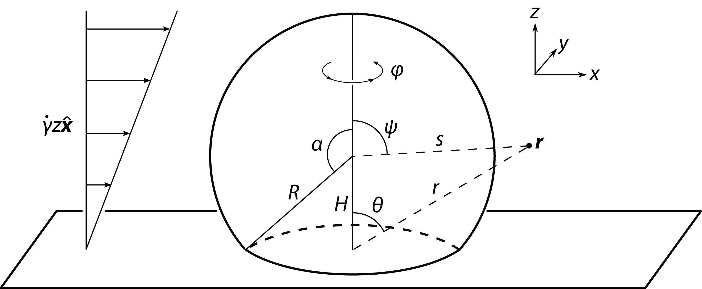
Figure 1: Geometry of the problem.

In what follows we non-dimensionalise space by $R$, velocities by $R\dot{\gamma}$ and volume pressures by $\dot{\gamma}^{2}\rho R^{2}$. Boundary conditions are then applied on $s=1$ and the imposed shear rate is unity. We also define $h\equiv H/R$, the effective height in this scaling. The external flows obey the unforced Stokes and incompressibility equations,

$$\kappa_{\pm}\nabla^{2}\bm{u}^{\pm}-\bm{\nabla}p^{\pm}=\bm{0},\qquad\bm{\nabla}\bm{\cdot}\bm{u}^{\pm}=0,$$ (1)

where $\kappa_{\pm}=\eta_{\pm}/\dot{\gamma}\rho R^{2}$. We impose far-field asymptotics, planar no-slip and radial no-penetration:

$$\bm{u}^{+}\sim z\hat{\bm{x}} \text{ as }r\rightarrow\infty,$$ (2)

$$\bm{u}^{\pm}=\bm{0} \text{ on }\theta=\math@atom{\pi}{\mathchoice{\hbox{$\displaystyle\pi$}}{\hbox{$\textstyle\pi$}}{\hbox{$\scriptstyle\pi$}}{\hbox{$\scriptscriptstyle\pi$}}}/2,$$ (3)

$$\bm{u}^{\pm}\bm{\cdot}\hat{\bm{s}}=0 \text{ on }s=1.$$ (4)

All three velocities must be continuous across the membrane,

$$\bm{u}^{+}=\bm{u}^{m}=\bm{u}^{-} \text{ on }s=1,$$ (5)

which, along with (3), implies the planar no-slip condition $\bm{u}^{m}=\bm{0}$ at $\psi=\alpha$.

In the absence of the membrane, we would only impose continuity of the bulk fluids’ normal stresses at the interface, but since membranes can support tension, the bulk stresses may be discontinuous. By assumption the membrane satisfies the Stokes equations and incompressibility constrained to the surface $s=1$. For a planar membrane this is simple (e.g.  Lubensky & Goldstein, 1996), but curvature induces an extra term. Henle & Levine (2010) (see also Henle et al., 2008) formulate the Stokes equations in terms of covariant derivatives on an arbitrary manifold, from which the membrane tension (equivalent to a two-dimensional pressure) may be eliminated by taking the curl, as in the familiar derivation of the vorticity equation. In our notation,

$$\hat{\bm{s}}\bm{\cdot}\bm{\nabla}\times[\hat{\nabla}^{2}\bm{u}^{m}+\bm{u}^{m}]+\hat{\bm{s}}\bm{\cdot}\bm{\nabla}\times\left[\frac{2\bm{e}^{+}_{\parallel}}{r_{+}}-\frac{2\bm{e}^{-}_{\parallel}}{r_{-}}\right]_{s=1}=0,\quad\hat{\bm{\nabla}}\bm{\cdot}\bm{u}^{m}=0,$$ (6)

where $\bm{e}^{\pm}_{\parallel}=e_{s\psi}\hat{\bm{\psi}}+e_{s\phi}\hat{\bm{\phi}}$ are the bulk fluids’ in-plane normal rates-of-strain, $\hat{\bm{\nabla}}$ denotes the gradient operator constrained to the surface $s=1$, and we define

$$r_{\pm}\equiv\frac{\eta_{m}}{R\eta_{\pm}}.$$ (7)

These are the non-dimensional form of the ‘Saffman-Delbrück’ lengths $\ell_{\pm}\equiv\eta_{m}/\eta_{\pm}$ (Saffman & Delbrück, 1975; Saffman, 1976; Henle & Levine, 2010), and are the parameters with which we control the membrane dynamics. Using the typical values $\eta_{\pm}\sim 10^{-2}\;\text{Poise}$ (water), $\eta_{m}\sim 10^{-7}-10^{-5}\;\text{Poise cm}$ (Camley et al., 2010) and $R\sim 1-100\;\math@atom{\mu}{\mathchoice{\hbox{$\displaystyle\mu$}}{\hbox{$\textstyle\mu$}}{\hbox{$\scriptstyle\mu$}}{\hbox{$\scriptscriptstyle\mu$}}}\text{m}$, we find relevant experimental ranges to be $r_{\pm}\sim 10^{-3}-10$.

2.2 Solution method

We will first construct a set of basis functions for the bulk fluids such that the planar no-slip condition (3) is automatically satisfied. A common approach to solving Stokes flow problems is to use Lamb’s solution (Happel & Brenner, 1991), and Ozarkar & Sangani (2008) showed that it is possible to write down a no-slip image system for each individual Lamb mode in the manner of the original solution of Blake (1971) for a simple Stokeslet. However, this becomes algebraically unwieldy, and we adopt a slightly different approach.

A method similar to using a Lamb expansion is to write down the solution in terms of Papkovich–Neuber potentials (Tran-Cong & Blake, 1982): if $\nabla^{2}\bm{A}=\bm{0}$ and $\nabla^{2}B=0$,

$$\bm{v} =\bm{\nabla}(\bm{r}\bm{\cdot}\bm{A}+B)-2\bm{A}, \quad p =2\eta\bm{\nabla}\bm{\cdot}\bm{A},$$ (8)

is a solution to the incompressible Stokes equations $\eta\nabla^{2}\bm{v}=\bm{\nabla}p$, $\bm{\nabla}\bm{\cdot}\bm{v}=0$. This reduces the problem to one of solving the vector and scalar harmonic equations. Shankar (2005) uses this representation to solve for Stokes flow inside a circular cone using three harmonic basis functions, one scalar and two vector. The scalar harmonic is the usual solution to Laplace’s equation in spherical coordinates,

$$B(\bm{r};\nu,m)=r^{\nu}e^{\mathrm{i}m\phi}P^{m}_{\nu}(\cos\theta),$$ (9)

where $\nu\in\mathbb{R}$ (since the solution need not be analytic in $z<0$) and $m\in\mathbb{Z}$, and $P^{m}_{\nu}$ are the generalised associated Legendre functions. Two independent vector harmonics can then be derived from $B$ as $\bm{A}_{1}=\hat{\bm{r}}\times\bm{\nabla}(rB)$ and $\bm{A}_{2}=B\hat{\bm{z}}$, which evaluate to

$$\bm{A}_{1}(\bm{r};\nu,m) =-r^{\nu}e^{\mathrm{i}m\phi}[m\csc\theta P^{m}_{\nu}(\cos\theta)\hat{\bm{\theta}}+\mathrm{i}{P^{m}_{\nu}}^{\prime}(\cos\theta)\hat{\bm{\phi}}],$$ (10)

$$\bm{A}_{2}(\bm{r};\nu,m) =r^{\nu}e^{\mathrm{i}m\phi}[\cos\theta P^{m}_{\nu}(\cos\theta)\hat{\bm{r}}-\sin\theta P^{m}_{\nu}(\cos\theta)\hat{\bm{\theta}}],$$ (11)

where primes indicate differentiation with respect to $\theta$. Since the only non-zero imposed velocity is simple shear flow we only need the $m=1$ mode, and can take the real part of all basis functions, whose $m$-dependence we henceforth omit. We also write $\mathcal{P}_{\nu}(x)\equiv P^{1}_{\nu}(x)$.

The next step is to find combinations of these harmonics such that the no-slip condition (3) is satisfied. In Shankar (2005) this is done by evaluating the velocity field on the cone using one unit of $B(\bm{r};\nu+1)$, $a$ units of $\bm{A}_{1}(\bm{r};\nu)$ and $b$ units of $\bm{A}_{2}(\bm{r};\nu)$. However, the case of a flat plane is a special one and solutions with no contribution from $B$ are possible, so here we must take an arbitrary $c$ units of $B(\bm{r};\nu+1)$; then (8) gives

$$v_{r} =r^{\nu}\cos\phi\left[c(\nu+1)\mathcal{P}_{\nu+1}+b(\nu-1)\cos\theta\,\mathcal{P}_{\nu}\right],$$ (12a)

$$v_{\theta} =r^{\nu}\cos\phi\left[c\mathcal{P}^{\prime}_{\nu+1}+2a\csc\theta\,\mathcal{P}_{\nu}+b\left\{\sin\theta\,\mathcal{P}_{\nu}+\cos\theta\,\mathcal{P}^{\prime}_{\nu}\right\}\right],$$ (12b)

$$v_{\phi} =-r^{\nu}\sin\phi\left[c\csc\theta\,\mathcal{P}_{\nu+1}+2a\mathcal{P}^{\prime}_{\nu}+b\cot\theta\,\mathcal{P}_{\nu}\right].$$ (12c)

(From here on, where unspecified the argument of $\mathcal{P}_{\nu}$ is $\cos\theta$.) It is simple to find that demanding $\bm{v}=\bm{0}$ at $\theta=\math@atom{\pi}{\mathchoice{\hbox{$\displaystyle\pi$}}{\hbox{$\textstyle\pi$}}{\hbox{$\scriptstyle\pi$}}{\hbox{$\scriptscriptstyle\pi$}}}/2$ leads to two possible conditions:

Either $$2a+b-(\nu+2)c=0 \mathcal{P}_{\nu+1}(0) =0,$$ and (13)

or $$a=c=0 \mathcal{P}_{\nu}(0) =0.$$ and (14)

The condition $\mathcal{P}_{\nu}(0)=0$ has solutions $\nu=0,2,4,\ldots$ and $\nu=-1,-3,-5,\ldots$. (Note that $\mathcal{P}_{0}\equiv\mathcal{P}_{-1}\equiv 0$.)

With this basis the general solution with no-slip on $z=0$ can be written

$$\bm{v}(r,\theta,\phi)=\sum_{\nu=-\infty}^{\infty}r^{\nu}[a_{\nu}\bm{F}_{\nu}(\theta,\phi)+b_{\nu}\bm{G}_{\nu}(\theta,\phi)+c_{\nu}\bm{H}_{\nu}(\theta,\phi)],$$ (15)

where the functions $\bm{F},\bm{G},\bm{H}$ may be read off from (12) as the coefficients of $a,b,c$ respectively. The coefficients must satisfy

$$2a_{\nu}+b_{\nu}-(\nu+2)c_{\nu}=0 \nu =1,3,5,\ldots,\nu=-2,-4,-6,\ldots,$$ for (16)

$$a_{\nu}=c_{\nu}=0 \nu =2,4,6,\ldots,\nu=-3,-5,-7,\ldots.$$ for (17)

These constraints can be incorporated directly into the expansion by writing

$$\bm{v}(r,\theta,\phi)=\sum_{\begin{subarray}{c}\nu=2,4,6,\ldots\\ \nu=-3,-5,\ldots\end{subarray}}r^{\nu}b_{\nu}\bm{G}_{\nu}(\theta,\phi)+\sum_{\begin{subarray}{c}\nu=1,3,5,\ldots\\ \nu=-2,-4,\ldots\end{subarray}}r^{\nu}[a_{\nu}\bm{F}^{(1)}_{\nu}(\theta,\phi)+c_{\nu}\bm{F}^{(2)}_{\nu}(\theta,\phi)]$$ (18)

where $\bm{F}^{(1)}_{\nu}=\bm{F}_{\nu}-2\bm{G}_{\nu}$ and $\bm{F}^{(2)}_{\nu}=\bm{H}_{\nu}+(\nu+2)\bm{G}_{\nu}$.

We now expand $\bm{u}^{-}$ and $\bm{U}^{+}$ in this fashion. Requiring regularity of $\bm{u}^{-}$ at $r=0$ implies that $a^{-}_{\nu},b^{-}_{\nu},c^{-}_{\nu}$ are non-zero only for $\nu>0$. Similarly, for $\bm{u}^{+}=z\hat{\bm{x}}+\bm{U}^{+}$ to satisfy the asymptotic condition (2) we must have $\bm{U}^{+}\rightarrow 0$ as $r\rightarrow\infty$ and so $a^{+}_{\nu},b^{+}_{\nu},c^{+}_{\nu}$ are non-zero only for $\nu<0$.

We now turn our attention to the flow on the membrane surface $s=1$. In Henle & Levine (2010) it is shown that the surface flow $\bm{u}^{m}(\bm{r})$ can be decomposed into a sum of incompressible shear modes $\bm{w}(\psi,\phi;\mu)=\bm{s}\times\bm{\nabla}\Phi(\psi,\phi;\mu)$ where the scalar functions $\Phi(\psi,\phi;\mu)$ are eigenfunctions of the Laplacian, $\nabla^{2}\Phi(\psi,\phi;\mu)=-\mu(\mu+1)\Phi(\psi,\phi;\mu)$. For the same reasons as in the bulk flow, we may take $\Phi(\psi,\phi;\mu)=\cos\phi\mathcal{P}_{\mu}(\cos\psi)$, whence

$$\bm{w}(\psi,\phi;\mu)=\frac{2}{\sin\psi}\mathcal{P}_{\mu}(\cos\psi)\cos\phi\,\hat{\bm{\psi}}-2\mathcal{P}^{\prime}_{\mu}(\cos\psi)\sin\phi\,\hat{\bm{\phi}}.$$ (19)

Given a mode spectrum $\{\mu_{n}\}$, expand the velocity as $\bm{u}^{m}(\psi,\phi)=\sum_{n}A_{n}\bm{w}(\psi,\phi;\mu_{n})$. Incompressibility is satisfied for each mode by construction. Then the membrane dynamics (6) become (Henle & Levine, 2010)

$$\sum_{n}A_{n}[2-\mu_{n}(\mu_{n}+1)]\mu_{n}(\mu_{n}+1)\Phi(\psi,\phi;\mu_{n})+\hat{\bm{s}}\bm{\cdot}\bm{\nabla}\times\left[\frac{2\bm{e}^{+}_{\parallel}}{r_{+}}-\frac{2\bm{e}^{-}_{\parallel}}{r_{-}}\right]_{s=1}=0.$$ (20)

There still remains the question of which modes $\mu$ to sum over. The ideal basis set would satisfy no-slip at $\psi=\alpha$ in the same way as the bulk fluid basis functions. For the membrane basis there is not enough freedom, so we can only choose one component to automatically be zero. We choose to set $u^{m}_{\psi}(\alpha,\phi;\mu)=0$ for all $\phi$, which implies

$$0=\mathcal{P}^{\prime}_{\mu}(\cos\alpha)=(1+\mu)\cot\alpha\mathcal{P}_{\mu}(\cos\alpha)-\mu\csc\alpha\mathcal{P}_{\mu+1}(\cos\alpha).$$ (21)

We can also take $\mu>0$ by the identity $\mathcal{P}_{-(\mu+1)}\equiv\mathcal{P}_{\mu}$. For the case $\alpha=\math@atom{\pi}{\mathchoice{\hbox{$\displaystyle\pi$}}{\hbox{$\textstyle\pi$}}{\hbox{$\scriptstyle\pi$}}{\hbox{$\scriptscriptstyle\pi$}}}/2$, i.e. a perfect hemisphere ($h=0$), this equation has exact solutions $\mu=1,3,5,\ldots$; if $\alpha>\math@atom{\pi}{\mathchoice{\hbox{$\displaystyle\pi$}}{\hbox{$\textstyle\pi$}}{\hbox{$\scriptstyle\pi$}}{\hbox{$\scriptscriptstyle\pi$}}}/2$, this must be solved numerically by a method such as Newton–Raphson to obtain the spectrum of allowed modes. Figure 2 shows streamlines of three different recirculatory modes for the hemispherical case, demonstrating the increase in number of circulation centres as the mode number increases. The same qualitative patterns persist for $h>0$.

Figure 2: Streamlines of recirculating modes for $h=0$, projected onto the $z$-plane.

We now have seven sets of coefficients to solve for in the expansions: $a^{\pm}_{\nu},b^{\pm}_{\nu},c^{\pm}_{\nu}$ for $\bm{u}^{\pm}$, and $A_{n}$ for $\bm{u}^{m}$. These will be determined by satisfying the simple boundary conditions (4) and (5), and the stress boundary condition (20). Each component of each boundary condition will only have $\phi$ dependence in the form of an overall factor of $\sin\phi$ or $\cos\phi$, so we may factor these out and need only satisfy boundary conditions for the $\psi$-dependent factors.

The complexity of the system does not lend itself easily to significant analytic progress, and so we choose to proceed via numerical methods to determine the coefficients. Our chosen solution method is the least-squares error minimisation procedure as outlined by Shankar (2005). The velocity expansions are truncated at orders $N_{1}$ and $N_{2}$ for the bulk and membrane velocities respectively – note that use of least-squares minimisation is crucial here, since any attempt to solve exactly for a finite set of coefficients will yield poorly-determined systems. The boundary conditions are to be satisfied on $0\leq\psi\leq\alpha$. Divide the interval $[\epsilon,\alpha]$ ($\epsilon\ll 1$) into $M$ equal subintervals, separated by points $\{\psi_{k}\}$. For each boundary condition $\mathcal{C}_{i}$ to be enforced, write $\varepsilon_{ik}$ for the error in satisfying that condition at $\psi_{k}$. Minimising $E^{2}=\sum_{i,k}\varepsilon_{ik}^{2}$ with respect to $a^{\pm}_{\nu},b^{\pm}_{\nu},c^{\pm}_{\nu},A_{n}$ then gives a linear system which can be solved for the coefficients. As $N_{1},N_{2},M\rightarrow\infty$ the coefficients quickly approach limiting values. (In what follows, we typically use magnitudes $N_{1},N_{2},M\sim O(100)$.) Care must be taken in satisfying the stress condition (20), since the stress becomes divergent in the neighbourhood of $\psi=\alpha$ due to the discontinuous geometry. To avoid this we truncate the collocation points $\{\psi_{k}\}$ a small distance before $\psi=\alpha$ for this condition.

Due to the choice of origin for the bulk fluid expansion, the system quickly becomes numerically unstable as $h$ increases due to divergences in $r^{\nu}$ for $\nu>0,r>1$ and $\nu<0,r<1$ in evaluating the velocity expansions on $s=1$. However, if the bulk velocity were expanded about the origin of the vesicle we would no longer have a basis set satisfying planar no-slip, and would have to enforce boundary conditions along the entire $y=z=0$ line as well, which would also possess highly divergent coefficients.

3 Results and discussion

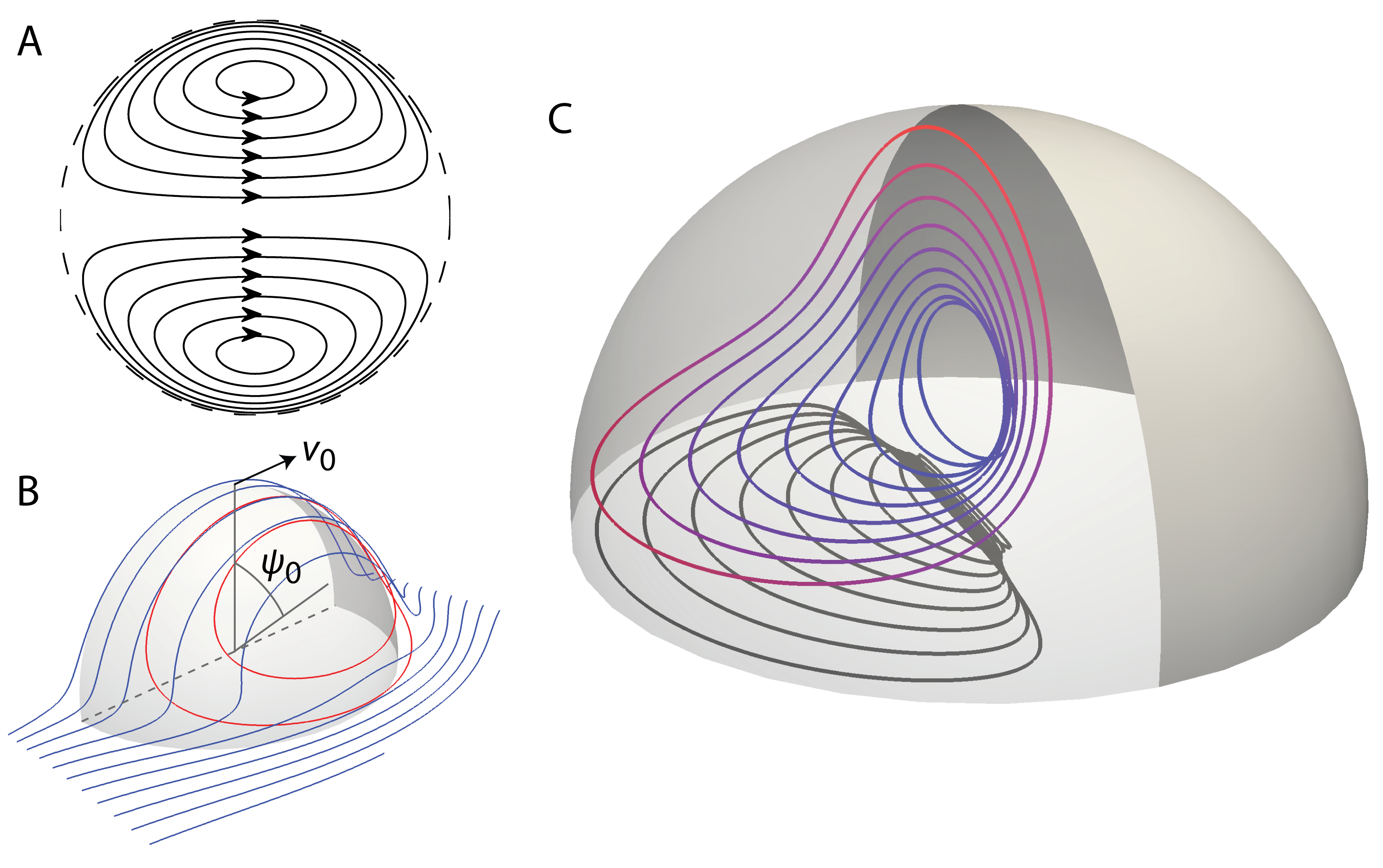
Figure 3: Streamlines for $r_{+}=r_{-}=0.01,h=0$. (a) Top view of membrane. (b) External flow, with closed streamlines in red. (c) Internal flow; brighter red indicates faster flow.

Figure 3a illustrates the typical flow induced on the surface of the vesicle. The closed, two-lobed symmetric recirculating patterns as observed by Vézy et al. (2007) are clearly reproduced, indicating a dynamical preference for motion rather than remaining stationary. The same structure persists for non-zero values of $h$ and for varying viscosity ratios $r_{\pm}$. The recirculatory flow of the membrane induces a flow inside the vesicle appearing to possess entirely closed streamlines, as illustrated in figure 3c. Similarly, the external flow shows regions of recirculation on either side of the membrane which also appear to contain closed streamlines (figure 3b).

The qualitative difference seen between this problem and that of an immiscible hemispherical droplet (Sugiyama & Sbragaglia, 2008) is due to the presence of the membrane. As described in §1, simple droplet flow permits both a surface-compressible structure and mass exchange with the interior. Due to the membrane structure, adhesion and incompressibility here, no such globally circulatory flow is possible.

The dynamical insistence on motion can be understood by the following argument. Consider the related problem of a free, spherical vesicle in uniform, unidirectional flow, for which it is known no membrane motion occurs. This problem is axisymmetric about the flow direction, and so the membrane experiences a tension constant along ‘lines of latitude’ perpendicular to the flow direction. Such a tension has no shearing component, and so the membrane is able to remain stationary. When the symmetry is broken by the introduction of the adhesive wall and the application of shear flow, the tension on the membrane is no longer uniform across ‘lines of latitude’. The membrane is unable to support this shear, forcing it to flow. The same symmetry-breaking effects have been observed in vesicle membrane flows driven by electric fields (Staykova et al., 2008) where a small field inhomogeneity develops shear stresses, causing the membrane to flow.

It should be noted that many surface-incompressible patterns are possible whilst remaining consistent with the symmetries of the problem; figure 2 shows the first three recirculatory modes of the membrane flow basis constructed in § 2.2. We observe that the flow adopts a pattern containing only two circulation centres rather than four or more, and pose the explanation that this is a consequence of dissipation reduction: the membrane is adopting the fewest number of topological ‘defects’ while still minimising dissipation within the bulk fluids.

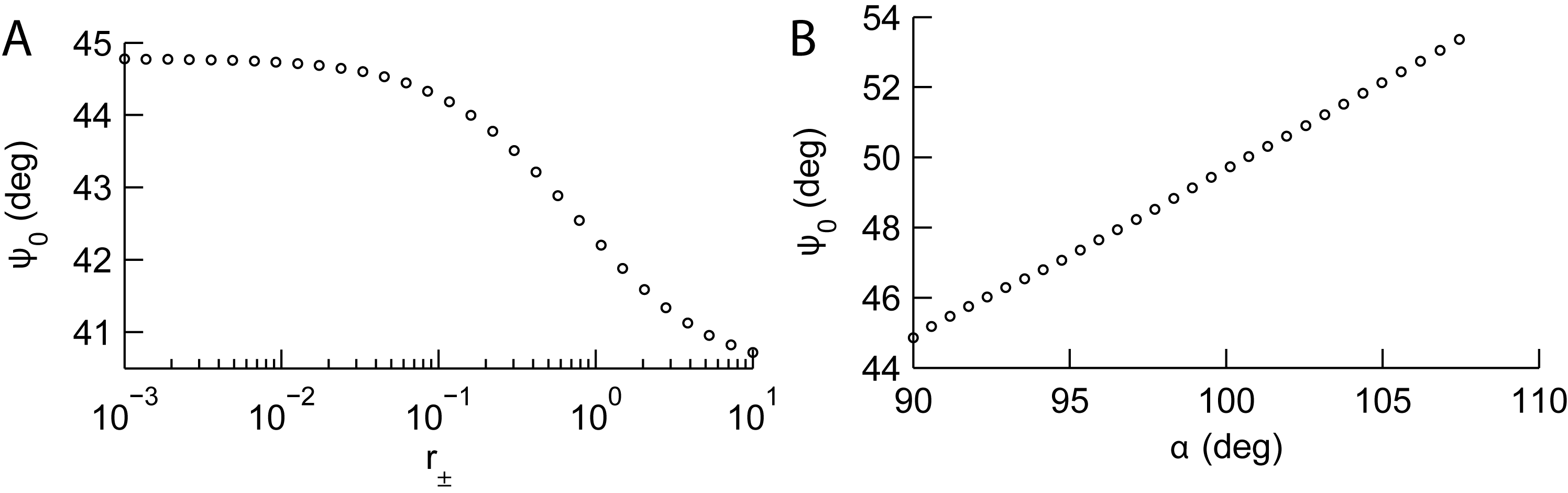
Figure 4: Dependence of the surface stagnation point angle on $r_{\pm}$ and $\alpha$. (a) $\alpha=\frac{\pi}{2}$, $r_{+}=r_{-}$, $10^{-3}\leq r_{\pm}\leq 10$, log scale in $r_{\pm}$. (b) $r_{+}=r_{-}=10^{-2}$, $0<h<0.3$.

As the membrane viscosity is increased through the physical range, the angle $\psi_{0}$ of the stagnation point from the vertical (see figure 3b) on either side shifts downwards, illustrated in figure 4a. The locations seen here are close to those observed by Vézy et al. (2007) (where their variable $\theta$ is equivalent to our $\frac{\pi}{2}-\psi$) for small values of $h$ (their $L/2R$ close to unity). We also observe that for $0<h<0.3$ the stagnation angle appears to scale linearly with the base angle $\alpha$, as might be expected (figure 4b).

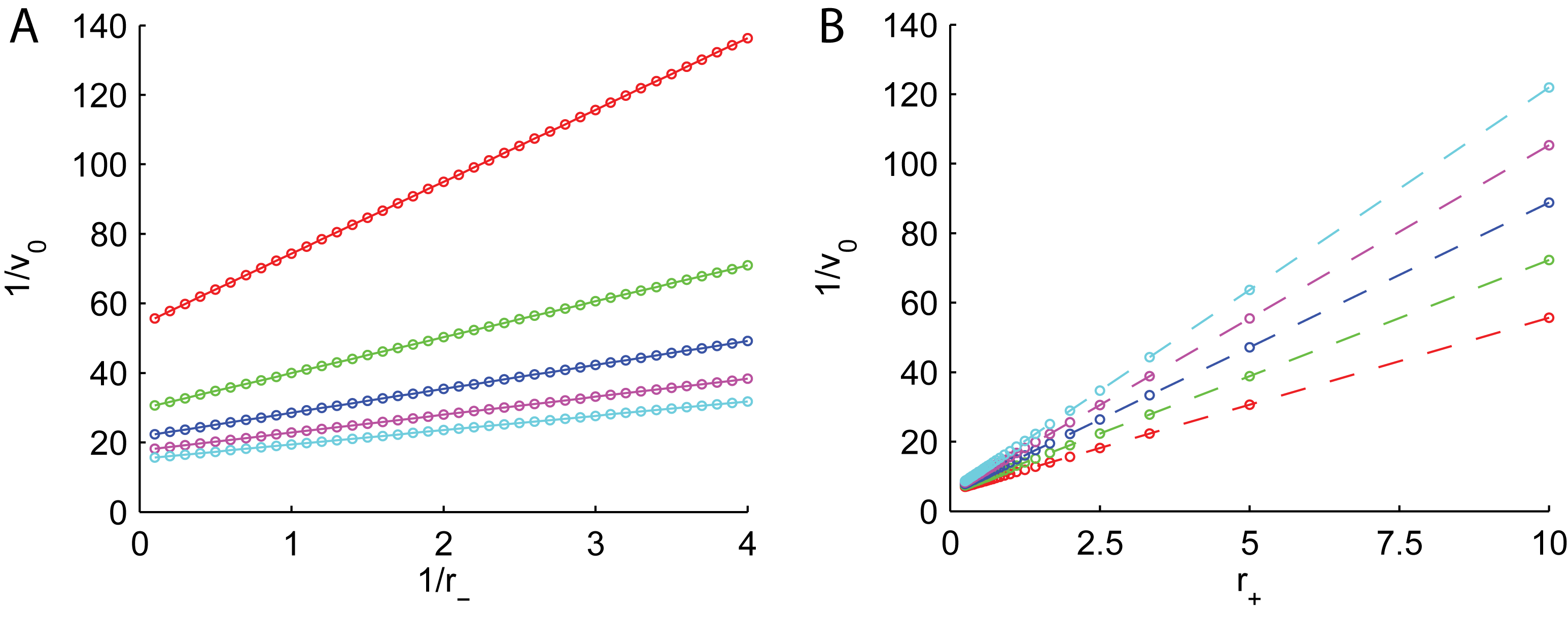
Figure 5: Linear dependence of $1/v_{0}$ on $1/r_{-}$ and $r_{+}$, at fixed values of $r_{+}$ and $r_{-}$, respectively. Top to bottom, (a) $r_{+}=10,5,3.33,2.5,2$, (b) $r_{-}=0.3,0.4,0.59,1.11,10$.

We now turn to the problem of experimentally determining the membrane viscosity $\eta_{m}$. Due to the order of magnitude of the physical constants involved, this is a difficult measurement to achieve. Dimova et al. (1999) proposed a method based upon measuring the fluctuations of a spherical particle stuck on or penetrating through a vesicle’s surface. While this method has been experimentally verified, and is perhaps simpler to initiate than encouraging vesicles to strongly adhere to substrates, it requires difficult measurements of microscopic parameters. An added benefit of the calculations presented here is a possible complementary method of membrane viscosity measurement based solely on the vesicle flow profiles, provided that the vesicle itself has not been affected by the adhesion process. Such velocities can be measured either by the defect-tracking method of Vézy et al. (2007) or by tracking small phase-separated patches of a second lipid species. Figure 5 suggests a fit of the apex velocity $v_{0}\equiv|\bm{v}^{m}(\psi=0)|$ (see figure 3b) with $r_{\pm}$ of the form

$$v_{0}=\frac{r_{-}}{Ar_{+}+Br_{+}r_{-}+Cr_{-}}$$ (22)

for a hemispherical membrane ($h=0$). Therefore given known bulk viscosities $\eta_{\pm}$, vesicle radius $R$ and measured apex velocity $v_{0}$, it would be possible to solve the above relationship and so predict the membrane viscosity $\eta_{m}$. Using $40\times 40$ regularly-spaced datapoints $(r_{+},r_{-})\in[0.25,10]^{2}$ we find an excellent fit for parameter values $A=2.054$, $B=4.718$, $C=5.803$, with root mean square error on the order of $10^{-4}$ and 95% confidence intervals $\sim\pm 0.001$. We expect such a relationship to persist for $h\neq 0$.

4 Conclusions

We have effected the theoretical solution of the problem of near-hemispherical lipid vesicles adhered to a flat substrate as experimentally investigated by Vézy et al. (2007). We demonstrated the presence of symmetric recirculating regions on the membrane and explained the qualitative difference from the membrane-less case. Additionally, the existence of closed streamlines both inside and outside the vesicle was shown. We then used knowledge of this system to suggest a new method for estimating membrane viscosities.

Throughout this work we have assumed the membrane remains spherical. For low shear rates, this assumption is valid; however, behaviour at higher shear rates is unlikely to remain stable. Li & Pozrikidis (1996) numerically studied the deformation of adhered immiscible liquid drops in shear flow and found a regime where the droplet would continue to deform over time. It is reasonable to suggest such deformations could occur in the case studied here, though the more complex surface and internal flow structure may lead to a different parameter phase space of deformations and instability.

Understanding the membrane flow has implications for other lipid membrane systems. One particular area where knowledge of the hydrodynamic behaviour of attached vesicles under shear flow is of importance is in the study of transient vesicle adhesion. If a vesicle loaded with binders comes into contact with a surface to which it may adhere, then the evolution of the contact area over time is dependent on the forcing experienced by the vesicle. Brochard-Wyart & de Gennes (2002) developed a dynamical adhesion force model based on the diffusion of binders on the membrane. However, if the vesicle is subjected to shear then free binders will be advected by the membrane flow which may significantly enhance or impair adhesive effects.

Possible future work in this area includes a more complex numerical study in order to accommodate all sizes of spherical cap (i.e. larger $h$), and experimental studies using the proposition of §3 to estimate membrane viscosities. It would also be interesting to study shear rates higher than those in Vézy et al. (2007) to understand whether buckling and deformation occur.

It is a pleasure to offer this contribution in honour of Tim Pedley’s 70th birthday. We thank P. Khuc Trong, P. Olla and J. Dunkel for helpful discussions and S. Ganguly for insights at an early stage of this work. This work was supported in part by the EPSRC and the European Research Council Advanced Investigator Grant 247333.

References

- Abkarian & Viallat (2008) Abkarian, M. & Viallat, A. 2008 Vesicles and red blood cells in shear flow. Soft Matter 4 (4), 653–657.
- Barthes-Biesel & Sgaier (1985) Barthes-Biesel, D. & Sgaier, H. 1985 Role of membrane viscosity in the orientation and deformation of a spherical capsule suspended in shear flow. J. Fluid Mech. 160, 119–135.
- Blake (1971) Blake, J. R. 1971 A note on the image system for a Stokeslet in a no-slip boundary. Math. Proc. Camb. Phil. Soc. 70, 303.
- Brochard-Wyart & de Gennes (2002) Brochard-Wyart, F. & de Gennes, P. G. 2002 Adhesion induced by mobile binders: dynamics. Proc. Natl. Acad. Sci. U.S.A. 99, 7854–7859.
- Camley et al. (2010) Camley, B. A., Esposito, C., Baumgart, T. & Brown, F. L. 2010 Lipid bilayer domain fluctuations as a probe of membrane viscosity. Biophys. J. 99, L44–46.
- Deschamps et al. (2009) Deschamps, J., Kantsler, V. & Steinberg, V. 2009 Phase diagram of single vesicle dynamical states in shear flow. Phys. Rev. Lett. 102 (11), 118105.
- Dimova et al. (1999) Dimova, R., Dietrich, C., Hadjiisky, A., Danov, K. & Pouligny, B. 1999 Falling ball viscosimetry of giant vesicle membranes: finite-size effects. Eur. Phys. J. B 12 (4), 589–598.
- Dussan V. (1987) Dussan V., E. B. 1987 On the ability of drops to stick to surfaces of solids. Part 3. The influences of the motion of the surrounding fluid on dislodging drops. J. Fluid Mech. 174, 381–397.
- Feng et al. (1989) Feng, S., Skalak, R. & Chien, S. 1989 Velocity distribution on the membrane of a tank-treading red blood cell. Bull. Math. Bio. 51 (4), 449–465.
- Happel & Brenner (1991) Happel, J. & Brenner, H. 1991 Low Reynolds number hydrodynamics: with special applications to particulate media. Kluwer Academic Print on Demand.
- Henle & Levine (2010) Henle, M. L. & Levine, A. J. 2010 Hydrodynamics in curved membranes: The effect of geometry on particulate mobility. Phys. Rev. E 81 (1), 011905.
- Henle et al. (2008) Henle, M. L., McGorty, R., Schofield, A. B., Dinsmore, A. D. & Levine, A. J. 2008 The effect of curvature and topology on membrane hydrodynamics. Europhys. Lett. 84, 48001.
- Kantsler et al. (2007) Kantsler, V., Segre, E. & Steinberg, V. 2007 Vesicle dynamics in time-dependent elongation flow: Wrinkling instability. Phys. Rev. Lett. 99 (17), 178102.
- Keller & Skalak (1982) Keller, S. R. & Skalak, R. 1982 Motion of a tank-treading ellipsoidal particle in a shear flow. J. Fluid Mech. 120, 27–47.
- Lebedev et al. (2007) Lebedev, V. V., Turitsyn, K. S. & Vergeles, S. S. 2007 Dynamics of nearly spherical vesicles in an external flow. Phys. Rev. Lett. 99 (21), 218101.
- Li & Pozrikidis (1996) Li, X. & Pozrikidis, C. 1996 Shear flow over a liquid drop adhering to a solid surface. J. Fluid Mech. 307, 167–190.
- Lorz et al. (2000) Lorz, B., Simson, R., Nardi, J. & Sackmann, E. 2000 Weakly adhering vesicles in shear flow: Tanktreading and anomalous lift force. Europhys. Lett. 51, 468.
- Lubensky & Goldstein (1996) Lubensky, D. K. & Goldstein, R. E. 1996 Hydrodynamics of monolayer domains at the air–water interface. Phys. Fluids 8 (4), 843–854.
- van de Meent et al. (2010) van de Meent, J.-W., Sederman, A. J., Gladden, L. F. & Goldstein, R. E. 2010 Measurement of cytoplasmic streaming in single plant cells by magnetic resonance velocimetry. J. Fluid Mech. 642, 5–14.
- Misbah (2006) Misbah, C. 2006 Vacillating breathing and tumbling of vesicles under shear flow. Phys. Rev. Lett. 96, 028104.
- Ozarkar & Sangani (2008) Ozarkar, S. S. & Sangani, A. S. 2008 A method for determining Stokes flow around particles near a wall or in a thin film bounded by a wall and a gas-liquid interface. Phys. Fluids 20, 063301.
- Pickard (1972) Pickard, W. F. 1972 Further observations on cytoplasmic streaming in Chara braunii. Can. J. Bot. 50, 703–711.
- Saffman (1976) Saffman, P. G. 1976 Brownian motion in thin sheets of viscous fluid. J. Fluid Mech. 73 (4), 593–602.
- Saffman & Delbrück (1975) Saffman, P. G. & Delbrück, M. 1975 Brownian motion in biological membranes. Proc. Natl. Acad. Sci. U.S.A. 72, 3111–3113.
- Seifert (1997) Seifert, U. 1997 Configurations of fluid membranes and vesicles. Adv. Phys. 46 (1), 13–137.
- Seifert (1999) Seifert, U. 1999 Fluid membranes in hydrodynamic flow fields: Formalism and an application to fluctuating quasispherical vesicles in shear flow. Eur. Phys. J. B 8, 405–415.
- Seifert & Langer (1993) Seifert, U. & Langer, S. A. 1993 Viscous modes of fluid bilayer membranes. Europhys. Lett. 23, 71.
- Shankar (2005) Shankar, P. N. 2005 Moffatt eddies in the cone. J. Fluid Mech. 539, 113–135.
- Staykova et al. (2008) Staykova, M., Lipowsky, R. & Dimova, R. 2008 Membrane flow patterns in multicomponent giant vesicles induced by alternating electric fields. Soft Matter 4 (11), 2168–2171.
- Sugiyama & Sbragaglia (2008) Sugiyama, K. & Sbragaglia, M. 2008 Linear shear flow past a hemispherical droplet adhering to a solid surface. J. Eng. Math. 62 (1), 35–50.
- Tran-Cong & Blake (1982) Tran-Cong, T. & Blake, J. R. 1982 General solutions of the Stokes’ flow equations. J. Math. Anal. Appl. 90 (1), 72–84.
- Verchot-Lubicz & Goldstein (2010) Verchot-Lubicz, J. & Goldstein, R. E. 2010 Cytoplasmic streaming enables the distribution of molecules and vesicles in large plant cells. Protoplasma 240, 99–107.
- Vézy et al. (2007) Vézy, C., Massiera, G. & Viallat, A. 2007 Adhesion induced non-planar and asynchronous flow of a giant vesicle membrane in an external shear flow. Soft Matter 3 (7), 844–851.
- Zhao & Shaqfeh (2011) Zhao, H. & Shaqfeh, E. S. G. 2011 The dynamics of a vesicle in simple shear flow. J. Fluid Mech. 674, 578–604.