Distributed Pareto Optimization via Diffusion Strategies

Abstract

We consider solving multi-objective optimization problems in a distributed manner by a network of cooperating and learning agents. The problem is equivalent to optimizing a global cost that is the sum of individual components. The optimizers of the individual components do not necessarily coincide and the network therefore needs to seek Pareto optimal solutions. We develop a distributed solution that relies on a general class of adaptive diffusion strategies. We show how the diffusion process can be represented as the cascade composition of three operators: two combination operators and a gradient descent operator. Using the Banach fixed-point theorem, we establish the existence of a unique fixed point for the composite cascade. We then study how close each agent converges towards this fixed point, and also examine how close the Pareto solution is to the fixed point. We perform a detailed mean-square error analysis and establish that all agents are able to converge to the same Pareto optimal solution within a sufficiently small mean-square-error (MSE) bound even for constant step-sizes. We illustrate one application of the theory to collaborative decision making in finance by a network of agents.

I Introduction

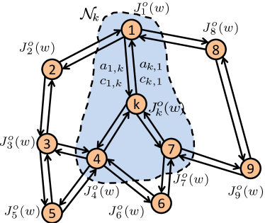
We consider solving a multi-objective optimization problem in a distributed manner over a network of $N$ cooperative learners (see Fig. 1). Each agent $k$ is associated with an individual cost function $J_{k}^{o}(w)$; and each of these costs may not be minimized at the same vector $w^{o}$. As such, we need to seek a solution that is “optimal” in some sense for the entire network. In these cases, a general concept of optimality known as Pareto optimality is useful to characterize how good a solution is. A solution $w^{o}$ is said to be Pareto optimal if there does not exist another vector $w$ that is able to improve (i.e., reduce) any particular cost, say, $J_{k}^{o}(w)$, without degrading (increasing) some of the other costs $\{J_{l}^{o}(w)\}_{l\neq k}$. To illustrate the idea of Pareto optimality, let

$$\mathcal{O} \triangleq\{(J_{1}^{o}(w),\ldots,J_{N}^{o}(w)):\;w\in\mathbb{W}\}\subseteq\mathbb{R}^{N}$$ (1)

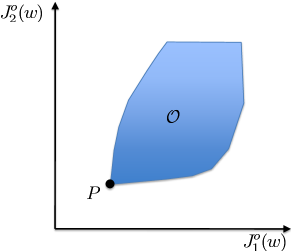
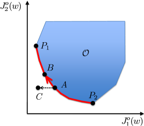
denote the set of achievable cost values, where $\mathbb{W}$ denotes the feasible set. Each point $P\in\mathcal{O}$ represents attained values for the cost functions $\{J_{l}^{o}(w)\}$ at a certain $w\in\mathbb{W}$. Let us consider the two-node case ($N=2$) shown in Fig. 2, where the shaded areas represent the set $\mathcal{O}$ for two situations of interest.

Figure 1: A network of $N$ cooperating agents; a cost function $J_{k}^{o}(w)$ is associated with each node $k$. The set of neighbors of node $k$ is denoted by ${\cal N}_{k}$ (including node $k$ itself); this set consists of all nodes with which node $k$ can share information.

In Fig. 2, both $J_{1}^{o}(w)$ and $J_{2}^{o}(w)$ achieve their minima at the same point $P=(J_{1}^{o}(w^{o}),J_{2}^{o}(w^{o}))$, where $w^{o}$ is the common minimizer. In comparison, in Fig. 2, $J_{1}^{o}(w)$ attains its minimum at point $P_{1}$, while $J_{2}^{o}(w)$ attains its minimum at point $P_{2}$, so that they do not have a common minimizer. Instead, all the points on the heavy red curve between points $P_{1}$ and $P_{2}$ are Pareto optimal solutions. For example, starting at point $A$ on the curve, if we want to reduce the value of $J_{1}^{o}(w)$ without increasing the value of $J_{2}^{o}(w)$, then we will need to move out of the achievable set $\mathcal{O}$. The alternative choice that would keep us on the curve is to move to another Pareto optimal point $B$, which would however increase the value of $J_{2}^{o}(w)$. In other words, we need to trade the value of $J_{2}^{o}(w)$ for $J_{1}^{o}(w)$. For this reason, the curve from $P_{1}$ to $P_{2}$ is called the optimal tradeoff curve (or optimal tradeoff surface if $N>2$) [2, p.183].

Figure 2: Optimal and Pareto optimal points for the case $N=2$: (Left) $P$ denotes the optimal point where both cost functions are minimized simultaneously and (Right) Pareto optimal points lie on the red boundary curve.

To solve for Pareto optimal solutions, a useful scalarization technique is often used to form an aggregate cost function that is the weighted sum of the component costs as follows:

$$J^{\mathrm{glob}}(w)=\sum_{l=1}^{N}\pi_{l}J_{l}^{o}(w)$$ (2)

where $\pi_{l}$ is a positive weight attached with the $l$th cost. It was shown in [2, pp.178–180] that the minimizer of (2) is Pareto optimal for the multi-objective optimization problem. Moreover, by varying the values of $\{\pi_{l}\}$, we are able to get different Pareto optimal points on the tradeoff curve. Observing that we can always define a new cost $J_{l}(w)$ by incorporating the weighting scalar $\pi_{l}$,

$$J_{l}(w)\triangleq\pi_{l}J_{l}^{o}(w)$$ (3)

it is sufficient for our future discussions to focus on aggregate costs of the following form:

$$\boxed{J^{\mathrm{glob}}(w)=\sum_{l=1}^{N}J_{l}(w)}$$ (4)

If desired, we can also add constraints to problem (4). For example, suppose there is additionally some constraint of the form $p_{k}^{T}w<b_{k}$ at node $k$, where $p_{k}$ is $M\times 1$ and $b_{k}$ is a scalar. Then, we can consider using barrier functions to convert the constrained optimization problem to an unconstrained problem [2, 3]. For example, we can redefine each cost $J_{k}(w)$ to be $J_{k}(w)\leftarrow J_{k}(w)+\phi(p_{k}^{T}w-b_{k})$, where $\phi(x)$ is a barrier function that penalizes values of $w$ that violate the constraint. Therefore, without loss of generality, we shall assume $\mathbb{W}=\mathbb{R}^{M}$ and only consider unconstrained optimization problems. Moreover, we shall assume the $\{J_{l}^{o}(w)\}$ are differentiable and, for each given set of positive weights $\{\pi_{l}\}$, the cost $J^{\mathrm{glob}}(w)$ in (2) or (4) is strongly convex so that the minimizer $w^{o}$ is unique [4]. Note that the new cost $J_{l}(w)$ in (3) depends on $\pi_{l}$ so that the $w^{o}$ that minimizes $J^{\mathrm{glob}}(w)$ in (4) also depends on $\{\pi_{l}\}$.

One of the most studied approaches to the distributed solution of such optimization problems is the incremental approach — see, e.g., [5, 6, 7, 8, 9, 10, 11, 12]. In this approach, a cyclic path is defined over the nodes and data are processed in a cyclic manner through the network until optimization is achieved. However, determining a cyclic path that covers all nodes is generally an NP-hard problem[13] and, in addition, cyclic trajectories are vulnerable to link and node failures. Another useful distributed optimization approach relies on the use of consensus strategies[5, 14, 15, 16, 17, 18, 19, 20]. In this approach, vanishing step-size sequences are used to ensure that agents reach consensus and agree about the optimizer in steady-state. However, in time-varying environments, diminishing step-sizes prevent the network from continuous learning; when the step-sizes die out, the network stops learning.

In [21], we generalized our earlier work on adaptation and learning over networks [22, 23] and developed diffusion strategies that enable the decentralized optimization of global cost functions of the form (4). In the diffusion approach, information is processed locally at the nodes and then diffused through a real-time sharing mechanism. In this manner, the approach is scalable, robust to node and link failures, and avoids the need for cyclic trajectories. In addition, compared to the aforementioned consensus solutions (such as those in [16, 19, 24]), the diffusion strategies we consider here employ constant (rather than vanishing) step-sizes in order to endow the resulting networks with continuous learning and tracking abilities. By keeping the step-sizes constant, the agents are able to track drifts in the underlying costs and in the location of the Pareto optimal solutions. One of the main challenges in the ensuing analysis becomes that of showing that the agents are still able to approach the Pareto optimal solution even with constant step-sizes; in this way, the resulting diffusion strategies are able to combine the two useful properties of optimality and adaptation.

In [21], we focused on the important case where all costs $\{J_{l}(w)\}$ share the same optimal solution $w^{o}$ (as was the case with Fig. 2); this situation arises when the agents in the network have a common objective and they cooperate to solve the problem of mutual interest in a distributed manner. Examples abound in biological networks where agents work together, for example, to locate food sources or evade predators[25], and in collaborative spectrum sensing[26], system identification[27], and learning applications[28]. In this paper, we develop the necessary theory to show that the same diffusion approach (described by (11)–(14) below) can be used to solve the more challenging multi-objective optimization problem, where the agents need to converge instead to a Pareto optimal solution. Such situations are common in the context of multi-agent decision making (see, e.g., [3] and also Sec. IV where we discuss one application in the context of collaborative decision in finance). To study this more demanding scenario, we first show that the proposed diffusion process can be represented as the cascade composition of three operators: two combination (aggregation) operators and one gradient-descent operator. Using the Banach fixed-point theorem[29, pp.299–303], we establish the existence of a unique fixed point for the composite cascade. We then study how close each agent in the network converges towards this fixed point, and also examine how close the Pareto solution is to the fixed point. We perform a detailed mean-square error analysis and establish that all agents are able to converge to the same Pareto optimal solution within a sufficiently small mean-square-error (MSE) bound. We illustrate the results by considering an example involving collaborative decision in financial applications.

Notation. Throughout the paper, all vectors are column vectors. We use boldface letters to denote random quantities (such as $\bm{u}_{k,i}$) and regular font to denote their realizations or deterministic variables (such as $u_{k,i}$). We use $\mathrm{diag}\{x_{1},\ldots,x_{N}\}$ to denote a (block) diagonal matrix consisting of diagonal entries (blocks) $x_{1},\ldots,x_{N}$, and use $\mathrm{col}\{x_{1},\ldots,x_{N}\}$ to denote a column vector formed by stacking $x_{1},\ldots,x_{N}$ on top of each other. The notation $x\preceq y$ means each entry of the vector $x$ is less than or equal to the corresponding entry of the vector $y$.

II Diffusion Adaptation Strategies

In [21], we motivated and derived diffusion strategies for distributed optimization, which are captured by the following general description:

$${\phi}_{k,i-1} =\displaystyle\sum_{l=1}^{N}a_{1,lk}{w}_{l,i-1}$$ (5)

$${\psi}_{k,i} =\displaystyle{\phi}_{k,i-1}-\mu_{k}\sum_{l=1}^{N}c_{lk}{\nabla}_{w}J_{l}({\phi}_{k,i-1})$$ (6)

$${w}_{k,i} =\displaystyle\sum_{l=1}^{N}a_{2,lk}{\psi}_{l,i}$$ (7)

where ${w}_{k,i}$ is the local estimate for $w^{o}$ at node $k$ and time $i$, $\mu_{k}$ is the step-size parameter used by node $k$, and $\{\phi_{k,i-1},\psi_{k,i}\}$ are intermediate estimates for $w^{o}$. Moreover, $\nabla_{w}J_{l}(\cdot)$ is the (column) gradient vector of $J_{l}(\cdot)$ relative to $w$. The non-negative coefficients $\{a_{1,lk}\}$, $\{c_{lk}\}$, and $\{a_{2,lk}\}$ are the $(l,k)$-th entries of matrices $A_{1}$, $C$, and $A_{2}$, respectively, and they are required to satisfy:

$$\left\{\begin{split}&A_{1}^{T}\mathds{1}=\mathds{1},\;A_{2}^{T}\mathds{1}=\mathds{1},\;C\mathds{1}=\mathds{1}\\ &a_{1,lk}=0,~{}a_{2,lk}=0,~{}c_{lk}=0\mathrm{~{}if~{}}l\notin\mathcal{N}_{k}\end{split}\right.$$ (8)

where $\mathds{1}$ denotes a vector with all entries equal to one. Note from (8) that the combination coefficients $\{a_{1,lk},a_{2,lk},c_{lk}\}$ are nonzero only for those $l\in\mathcal{N}_{k}$. Therefore, the sums in (5)–(7) are confined within the neighborhood of node $k$. Condition (8) requires the combination matrices $\{A_{1},A_{2}\}$ to be left-stochastic, while $C$ is right-stochastic. We therefore note that each node $k$ first aggregates the existing estimates from its neighbors through (5) and generates the intermediate estimate $\phi_{k,i-1}$. Then, node $k$ aggregates gradient information from its neighborhood and updates $\phi_{k,i-1}$ to $\phi_{k,i}$ through (6). All other nodes in the network are performing these same steps simultaneously. Finally, node $k$ aggregates the estimates $\{\phi_{l,i}\}$ through step (7) to update its weight estimate to $w_{k,i}$.

Algorithm (5)–(7) can be simplified to several special cases for different choices of the matrices $\{A_{1},A_{2},C\}$. For example, the choice $A_{1}=I$, $A_{2}=A$ and $C=I$ reduces to the adapt-then-combine (ATC) strategy that has no exchange of gradient information [22, 21, 23, 30]:

$$\boxed{\begin{array}[]{l}\psi_{k,i}=\displaystyle w_{k,i-1}-\mu_{k}\nabla_{w}J_{k}(w_{k,i-1})\\ w_{k,i}=\displaystyle\sum_{l\in\mathcal{N}_{k}}a_{lk}\psi_{l,i}\end{array}}\;\;(\mathrm{ATC},\;C=I)$$ (11)

while the choice $A_{1}=A$, $A_{2}=I$ and $C=I$ reduces to the combine-then-adapt (CTA) strategy, where the order of the combination and adaptation steps are reversed relative to (11) [22, 23, 30]:

$$\boxed{\begin{array}[]{l}\psi_{k,i\!-\!1}=\displaystyle\sum_{l\in\mathcal{N}_{k}}a_{lk}w_{l,i-1}\\ w_{k,i}=\displaystyle\psi_{k,i-1}-\mu_{k}\nabla_{w}J_{k}(\psi_{k,i-1})\end{array}}\;\;(\mathrm{CTA},\;C=I)$$ (14)

Furthermore, if in the CTA implementation (14) we enforce $A$ to be doubly stochastic, replace $\nabla_{w}J_{k}(\cdot)$ by a subgradient, and use a time-decaying step-size parameter ($\mu_{k}(i)\rightarrow 0$), then we obtain the unconstrained version used by [24]. In the sequel, we continue with the general recursions (5)–(7), which allow us to examine the convergence properties of several algorithms in a unified manner. The challenge we encounter now is to show that this same class of algorithms can still optimize the cost (4) in a distributed manner when the individual costs $\{J_{l}(w)\}$ do not necessarily have the same minimizer. This is actually a demanding task, as the analysis in the coming sections reveals, and we need to introduce novel analysis techniques to be able to handle this general case.

III Performance Analysis

III-A Modeling Assumptions

In most situations in practice, the true gradient vectors needed in (6) are not available. Instead, perturbed versions are available, which we model as

$$\widehat{\nabla_{w}J_{l}}(\bm{w})=\nabla_{w}J_{l}(\bm{w})+\bm{v}_{l,i}(\bm{w})$$ (15)

where the random noise term, $\bm{v}_{l,i}(\bm{w})$, may depend on $\bm{w}$ and will be required to satisfy certain conditions given by (20)–(21). We refer to the perturbation in (15) as gradient noise. Using (15), the diffusion algorithm (5)–(7) becomes the following, where we are using boldface letters for various quantities to highlight the fact that they are now stochastic in nature due to the randomness in the noise component:

$$\bm{\phi}_{k,i-1} =\displaystyle\sum_{l=1}^{N}a_{1,lk}\bm{w}_{l,i-1}$$ (16)

$$\bm{\psi}_{k,i} =\displaystyle\bm{\phi}_{k,i-1}-\mu_{k}\sum_{l=1}^{N}c_{lk}\big{[}{\nabla}_{w}J_{l}(\bm{\phi}_{k,i-1})+\bm{v}_{l,i}(\bm{\phi}_{k,i-1})\big{]}$$ (17)

$$\bm{w}_{k,i} =\displaystyle\sum_{l=1}^{N}a_{2,lk}\bm{\psi}_{l,i}$$ (18)

Using (16)–(18), we now proceed to examine the mean-square performance of the diffusion strategies. Specifically, in the sequel, we study: (i) how fast and (ii) how close the estimator $\bm{w}_{k,i}$ at each node $k$ approaches the Pareto-optimal solution $w^{o}$ in the mean-square-error sense. We establish the convergence of all nodes towards the same Pareto-optimal solution within a small MSE bound. Since we are dealing with individual costs that may not have a common minimizer, the approach we employ to examine the convergence properties of the diffusion strategy is fundamentally different from [21]; we follow a system-theoretic approach and call upon the fixed-point theorem for contractive mappings[29, pp.299–303].

To proceed with the analysis, we introduce the following assumptions on the cost functions and gradient noise. As explained in [21], these conditions are weaker than similar conditions in the literature of distributed optimization; in this way, our convergence and performance results hold under more relaxed conditions than usually considered in the literature.

Assumption 1 (Bounded Hessian).

Each component cost function $J_{l}(w)$ has a bounded Hessian matrix, i.e., there exist nonnegative real numbers $\lambda_{l,\min}$ and $\lambda_{l,\max}$ such that, for each $k=1,\ldots,N$:

$$\lambda_{l,\min}I_{M}\leq\nabla_{w}^{2}J_{l}(w)\leq\lambda_{l,\max}I_{M}$$ (19)

with $\sum_{l=1}^{N}c_{lk}\lambda_{l,\min}>0$. ∎

Assumption 2 (Gradient noise).

There exist $\alpha\geq 0$ and $\sigma_{v}^{2}\geq 0$ such that, for all $\bm{w}\in\mathcal{F}_{i-1}$:

$$\mathbb{E}\left\{\bm{v}_{l,i}(\bm{w})\;|\;\mathcal{F}_{i-1}\right\}=0$$ (20)

$$\mathbb{E}\left\{\|\bm{v}_{l,i}(\bm{w})\|^{2}\right\}\leq\alpha\cdot\mathbb{E}\|\nabla_{w}J_{l}(\bm{w})\|^{2}+\sigma_{v}^{2}$$ (21)

for all $i,l$, where $\mathcal{F}_{i-1}$ denotes the past history of estimators $\{\bm{w}_{k,j}\}$ for $j\leq i-1$ and all $k$. ∎

If we choose $C=I$, then Assumption 1 implies that the cost functions $\{J_{l}(w)\}$ are strongly convex. This condition can be guaranteed by adding small regularization terms. For example, we can convert a non-strongly convex function $J_{l}^{\prime}(w)$ to a strongly convex one by redefining $J_{l}(w)$ as $J_{l}(w)\leftarrow J_{l}(w)+\epsilon\|w\|^{2}$, where $\epsilon>0$ is a small regularization factor. We further note that, assumption (21) is a mix of the “relative random noise” and “absolute random noise” model usually assumed in stochastic approximation [4]. Condition (21) implies that the gradient noise grows when the estimate is away from the optimum (large gradient). Condition (21) also states that even when the gradient vector is zero, there is still some residual noise variance $\sigma_{v}^{2}$.

III-B Diffusion Adaptation Operators

To analyze the performance of the diffusion adaptation strategies, we first represent the mappings performed by (16)–(18) in terms of useful operators.

Definition 1 (Combination Operator).

Suppose $x=\mathrm{col}\{x_{1},\ldots,x_{N}\}$ is an arbitrary $N\times 1$ block column vector that is formed by stacking $M\times 1$ vectors $x_{1},\ldots,x_{N}$ on top of each other. The combination operator $T_{A}:\mathbb{R}^{MN}\rightarrow\mathbb{R}^{MN}$ is defined as the linear mapping:

$$T_{A}(x)\triangleq(A^{T}\otimes I_{M})\;x$$ (22)

where $A$ is an $N\times N$ left stochastic matrix, and $\otimes$ denotes the Kronecker product operation. ∎

Definition 2 (Gradient-Descent Operator).

Consider the same $N\times 1$ block column vector $x$. Then, the gradient-descent operator $T_{G}:\mathbb{R}^{MN}\rightarrow\mathbb{R}^{MN}$ is the nonlinear mapping defined by:

$$T_{G}(x)\triangleq\begin{bmatrix}x_{1}-\mu_{1}\sum_{l=1}^{N}c_{l1}\nabla_{w}J_{l}(x_{1})\\ \vdots\\ x_{N}-\mu_{N}\sum_{l=1}^{N}c_{lN}\nabla_{w}J_{l}(x_{N})\end{bmatrix}$$ (23)

∎

Definition 3 (Power Operator).

Consider the same $N\times 1$ block vector $x$. The power operator $P:\mathbb{R}^{MN}\rightarrow\mathbb{R}^{N}$ is defined as the mapping:

$$P[x]\triangleq\mathrm{col}\{\|x_{1}\|^{2},\ldots,\|x_{N}\|^{2}\}$$ (24)

where $\|\cdot\|$ denotes the Euclidean norm of a vector. ∎

We will use the power operator to study how error variances propagate after a specific operator $T_{A}(\cdot)$ or $T_{G}(\cdot)$ is applied to a random vector. We remark that we are using the notation “$P[\cdot]$” rather than “$P(\cdot)$” to highlight the fact that $P$ is a mapping from $\mathbb{R}^{MN}$ to a lower dimensional space $\mathbb{R}^{N}$. In addition to the above three operators, we define the following aggregate vector of gradient noise that depends on the state $x$:

$$\bm{v}(x)\triangleq\!-\mathrm{col}\Big{\{}\!\mu_{1}\!\sum_{l=1}^{N}c_{l1}\bm{v}_{l}(x_{1}),\ldots,\mu_{N}\!\sum_{l=1}^{N}c_{lN}\bm{v}_{l}(x_{N})\!\Big{\}}$$ (25)

With these definitions, we can now represent the two combination steps (16) and (18) as two combination operators $T_{A_{1}}(\cdot)$ and $T_{A_{2}}(\cdot)$. We can also represent the adaptation step (17) by a gradient-descent operator perturbed by the noise operator (25):

$$\widehat{\bm{T}}_{G}(x)\triangleq T_{G}(x)+\bm{v}(x)$$ (26)

We can view $\widehat{\bm{T}}_{G}(x)$ as a random operator that maps each input $x\in\mathbb{R}^{MN}$ into an $\mathbb{R}^{MN}$ random vector, and we use boldface letter to highlight this random nature. Let

$$\bm{w}_{i}\triangleq\mathrm{col}\{\bm{w}_{1,i},\bm{w}_{2,i},\ldots,\bm{w}_{N,i}\}$$ (27)

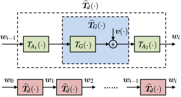
denote the vector that collects the estimators across all nodes. Then, the overall diffusion adaptation steps (16)–(18) that update $\bm{w}_{i-1}$ to $\bm{w}_{i}$ can be represented as a cascade composition of three operators:

$$\widehat{\bm{T}}_{d}(\cdot)\triangleq T_{A_{2}}\circ\widehat{\bm{T}}_{G}\circ T_{A_{1}}(\cdot)$$ (28)

where we use $\circ$ to denote the composition of any two operators, i.e., $T_{1}\circ T_{2}(x)\triangleq T_{1}(T_{2}(x))$. If there is no gradient noise, then the diffusion adaptation operator (28) reduces to

$$T_{d}(\cdot)\triangleq T_{A_{2}}\circ T_{G}\circ T_{A_{1}}(\cdot)$$ (29)

In other words, the diffusion adaptation over the entire network with and without gradient noise can be described in the following compact forms:

$$\bm{w}_{i} =\widehat{\bm{T}}_{d}(\bm{w}_{i-1})$$ (30)

$$w_{i} =T_{d}(w_{i-1})$$ (31)

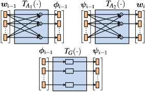
Fig. 3(a) illustrates the role of the combination operator $T_{A}(\cdot)$ (combination steps) and the gradient-descent operator $T_{G}(\cdot)$ (adaptation step). The combination operator $T_{A}(\cdot)$ aggregates the estimates from the neighborhood (social learning), while the gradient-descent operator $T_{G}(\cdot)$ incorporates information from the local gradient vector (self-learning). In Fig. 3(b), we show that each diffusion adaptation step can be represented as the cascade composition of three operators, with perturbation from the gradient noise operator.

(a) $T_{A_{1}}(\cdot)$, $T_{A_{2}}(\cdot)$ and $T_{G}(\cdot)$.

(b) Cascade representation of diffusion adaptation.

Figure 3: Representation of the diffusion adaptation strategy (16)–(18) in terms of operators. Each diffusion adaptation step can be viewed as a cascade composition of three operators: $T_{A_{1}}(\cdot)$, $T_{G}(\cdot)$, and $T_{A_{2}}(\cdot)$ with gradient perturbation $\bm{v}(\cdot)$. If $\bm{v}(\cdot)=0$, then $\widehat{\bm{T}}_{d}(\cdot)$ becomes $T_{d}(\cdot)$.

Next, in Lemma 1, we examine some of the properties of the operators $\{T_{A_{1}},T_{A_{2}},T_{G}\}$, which are proved in Appendix A.

Lemma 1 (Useful Properties).

Consider $N\times 1$ block vectors $x=\mathrm{col}\{x_{1},\ldots,x_{N}\}$ and $y=\mathrm{col}\{y_{1},\ldots,y_{N}\}$ with $M\times 1$ entries $\{x_{k},y_{k}\}$. Then, the operators $T_{A}(\cdot)$, $T_{G}(\cdot)$ and $P[\cdot]$ satisfy the following properties:

1. (Linearity): $T_{A}(\cdot)$ is a linear operator.

2. (Nonnegativity): $P[x]\succeq 0$.

3. (Scaling): For any scalar $a\in\mathbb{R}$, we have

   $$P[ax]=a^{2}P[x]$$ (32)

4. (Convexity): suppose $x^{(1)},\ldots,x^{(K)}$ are $N\times 1$ block vectors formed in the same manner as $x$, and let $a_{1},\ldots,a_{K}$ be non-negative real scalars that add up to one. Then,

   $$P[a_{1}x^{(1)} +\cdots+a_{K}x^{(K)}]\preceq a_{1}P[x^{(1)}]+\cdots+a_{K}P[x^{(K)}]$$ (33)

5. (Additivity): Suppose $\bm{x}=\mathrm{col}\{\bm{x}_{1},\ldots,\bm{x}_{N}\}$ and $\bm{y}=\mathrm{col}\{\bm{y}_{1},\ldots,\bm{y}_{N}\}$ are $N\times 1$ block random vectors that satisfy $\mathbb{E}\bm{x}_{k}^{T}\bm{y}_{k}=0$ for $k=1,\ldots,N$. Then,

   $$\mathbb{E}P[\bm{x}+\bm{y}]=\mathbb{E}P[\bm{x}]+\mathbb{E}P[\bm{y}]$$ (34)

6. (Variance relations):

   $$P[T_{A}(x)]\preceq A^{T}P[x]$$ (35)

   $$P[T_{G}(x)-T_{G}(y)]\preceq\Gamma^{2}P[x-y]$$ (36)

   where

   $$\Gamma \triangleq\mathrm{diag}\{\gamma_{1},\ldots,\gamma_{N}\}$$ (37)

   $$\gamma_{k} \triangleq\max\{|1-\mu_{k}\sigma_{k,\max}|,\;|1-\mu_{k}\sigma_{k,\min}|\}$$ (38)

   $$\sigma_{k,\min} \triangleq\sum_{l=1}^{N}c_{lk}\lambda_{l,\min},\;\sigma_{k,\max}\triangleq\sum_{l=1}^{N}c_{lk}\lambda_{l,\max}$$ (39)

7. (Block Maximum Norm): The $\infty-$norm of $P[x]$ is the squared block maximum norm of $x$:

   $$\|P[x]\|_{\infty}=\|x\|_{b,\infty}^{2}\triangleq\big{(}\max_{1\leq k\leq N}\|x_{k}\|\big{)}^{2}$$ (40)

8. (Preservation of Inequality): Suppose vectors $x$, $y$ and matrix $F$ have nonnegative entries, then $x\preceq y$ implies $Fx\preceq Fy$. ∎

III-C Transient Analysis

Using the operator representation developed above, we now analyze the transient behavior of the diffusion algorithm (16)–(18). From Fig. 3(b) and the previous discussion, we know that the stochastic recursion $\bm{w}_{i}=\widehat{\bm{T}}_{d}(\bm{w}_{i-1})$ is a perturbed version of the noise-free recursion $w_{i}=T_{d}(w_{i-1})$. Therefore, we first study the convergence of the noise free recursion, and then analyze the effect of gradient perturbation on the stochastic recursion.

Intuitively, if recursion $w_{i}=T_{d}(w_{i-1})$ converges, then it should converge to a vector $w_{\infty}$ that satisfies

$$w_{\infty}=T_{d}(w_{\infty})$$ (41)

In other words, the vector $w_{\infty}$ should be a fixed point of the operator $T_{d}(\cdot)$[29, p.299]. We need to answer four questions pertaining to the fixed point. First, does the fixed point exist? Second, is it unique? Third, under which condition does the recursion $w_{i}=T_{d}(w_{i-1})$ converge to the fixed point? Fourth, how far is the fixed point $w_{\infty}$ away from the minimizer $w^{o}$ of (4)? We answer the first two questions using the Banach Fixed Point Theorem (Contraction Theorem) [29, pp.2–9, pp.299–300]. Afterwards, we study convergence under gradient perturbation. The last question will be considered in the next subsection.

Definition 4 (Metric Space).

A set $X$, whose elements we shall call points, is said to be a metric space if we can associate a real number $d(p,q)$ with any two points $p$ and $q$ of $X$, such that

1. $d(p,q)>0$ if $p\neq q$; $d(p,p)=0$;

2. $d(p,q)=d(q,p)$;

3. $d(p,q)\leq d(p,r)+d(r,q)$, for any $r\in X$.

Any function $d(p,q)$ with these three properties is called a distance function, or a metric, and we denote a metric space $X$ with distance $d(\cdot,\cdot)$ as $(X,d)$. ∎

Definition 5 (Contraction).

Let $(X,d)$ be a metric space. A mapping $T:X\longrightarrow X$ is called a contraction on $X$ if there is a positive real number $\delta<1$ such that $d(T(x),T(y))\leq\delta\cdot d(x,y)$ for all $x,y\in X$

Lemma 2 (Banach Fixed Point Theorem[29]).

Consider a metric space $(X,d)$, where $X\neq\emptyset$. Suppose that $X$ is complete and let $T:X\rightarrow X$ be a contraction. Then, $T$ has precisely one fixed point. ∎

As long as we can prove that the diffusion operator $T_{d}(\cdot)$ is a contraction, i.e., for any two points $x,y\in\mathbb{R}^{MN}$, after we apply the operator $T_{d}(\cdot)$, the distance between $T_{d}(x)$ and $T_{d}(y)$ scales down by a scalar that is uniformly bounded away from one, then the fixed point $w_{\infty}$ defined in (41) exists and is unique. We now proceed to show that $T_{d}(\cdot)$ is a contraction operator in $X=\mathbb{R}^{MN}$ when the step-size parameters $\{\mu_{k}\}$ satisfy certain conditions.

Theorem 1 (Fixed Point).

Suppose the step-size parameters $\{\mu_{k}\}$ satisfy the following conditions

$$0<\mu_{k}<\frac{2}{\sigma_{k,\max}},\qquad k=1,2,\ldots,N$$ (42)

Then, there exists a unique fixed point $w_{\infty}$ for the unperturbed diffusion operator $T_{d}(\cdot)$ in (29).

Proof.

Let $x=\mathrm{col}\{x_{1},\ldots,x_{N}\}\in\mathbb{R}^{MN\times 1}$ be formed by stacking $M\times 1$ vectors $x_{1},\ldots,x_{N}$ on top of each other. Similarly, let $y=\mathrm{col}\{y_{1},\ldots,y_{N}\}$. The distance function $d(x,y)$ that we will use is induced from the block maximum norm (40): $d(x,y)=\|x-y\|_{b,\infty}=\max_{1\leq k\leq N}\|x_{k}-y_{k}\|$. From the definition of the diffusion operator $T_{d}(\cdot)$ in (29), we have

$$P[T_{d}(x)-T_{d}(y)] \overset{(a)}{=}P\big{[}T_{A_{2}}\big{(}T_{G}\circ T_{A_{1}}(x)-T_{G}\circ T_{A_{1}}(y)\big{)}\big{]}$$

$$\overset{(b)}{\preceq}A_{2}^{T}P\big{[}T_{G}\circ T_{A_{1}}(x)-T_{G}\circ T_{A_{1}}(y)\big{]}$$

$$\overset{(c)}{\preceq}A_{2}^{T}\Gamma^{2}P[T_{A_{1}}(x)-T_{A_{1}}(y)]$$

$$\overset{(d)}{=}A_{2}^{T}\Gamma^{2}P[T_{A_{1}}(x-y)]$$

$$\overset{(e)}{\preceq}A_{2}^{T}\Gamma^{2}A_{1}^{T}P[x-y]$$ (43)

where steps (a) and (d) are because of the linearity of $T_{A_{1}}(\cdot)$ and $T_{A_{2}}(\cdot)$, steps (b) and (e) are because of the variance relation property (35), and step (c) is due to the variance relation property (36). Taking the $\infty-$norm of both sides of (III-C), we have

$$\|P[T_{d}(x)-T_{d}(y)]\|_{\infty} \leq\|A_{2}^{T}\Gamma^{2}A_{1}^{T}\|_{\infty}\cdot\|P[x-y]\|_{\infty}$$

$$\leq\|\Gamma\|_{\infty}^{2}\cdot\|P[x-y]\|_{\infty}$$ (44)

where, in the second inequality, we used the fact that $\|A_{1}^{T}\|_{\infty}=\|A_{2}^{T}\|_{\infty}=1$ since $A_{1}^{T}$ and $A_{2}^{T}$ are right-stochastic matrices. Using property (40), we can conclude from (III-C) that: $\|T_{d}(x)-T_{d}(y)\|_{b,\infty}\leq\|\Gamma\|_{\infty}\cdot\|x-y\|_{b,\infty}$. Therefore, the operator $T_{d}(\cdot)$ is a contraction if $\|\Gamma\|_{\infty}<1$, which, by substituting (37)–(38), becomes

$$|1-\mu_{k}\sigma_{k,\max}|<1,\quad|1-\mu_{k}\sigma_{k,\min}|<1,\quad k=1,\ldots,N$$

and we arrive at the condition (42) on the step-sizes In other words, if condition (42) holds for each $k=1,\ldots,N$, then $T_{d}(\cdot)$ is a contraction operator. By Lemma 2, the operator $T_{d}(\cdot)$ will have a unique fixed point $w_{\infty}$ that satisfies equation (41). ∎

Given the existence and uniqueness of the fixed point, the third question to answer is if recursion $w_{i}=T_{d}(w_{i-1})$ converges to this fixed point. The answer is affimative under (42). However, we are not going to study this question separately. Instead, we will analyze the convergence of the more demanding noisy recursion (30). Therefore, we now study how fast and how close the successive estimators $\{\bm{w}_{i}\}$ generated by recursion (30) approach $w_{\infty}$. Once this issue is addressed, we will then examine how close $w_{\infty}$ is to the desired $w^{o}$. Introduce the following mean-square-perturbation (MSP) vector at time $i$:

$$\mathrm{MSP}_{i} \triangleq\mathbb{E}P[\bm{w}_{i}-w_{\infty}]$$ (45)

The $k$-th entry of $\mathrm{MSP}_{i}$ characterizes how far away the estimate $\bm{w}_{k,i}$ at node $k$ and time $i$ is from $w_{k,\infty}$ in the mean-square sense. To study the closeness of $\bm{w}_{i}$ to $w_{\infty}$, we shall study how the quantity $\mathrm{MSP}_{i}$ evolves over time. By (30), (41) and the definitions of $\widehat{\bm{T}}_{d}(\cdot)$ and $T_{d}(\cdot)$ in (28) and (29), we obtain

$$\mathrm{MSP}_{i} =\mathbb{E}P[\bm{w}_{i}-w_{\infty}]$$

$$\quad=\mathbb{E}P\big{[}T_{A_{2}}\circ\widehat{\bm{T}}_{G}\circ T_{A_{1}}(\bm{w}_{i-1})-T_{A_{2}}\circ T_{G}\circ T_{A_{1}}(w_{\infty})\big{]}$$

$$\quad\overset{(a)}{=}\mathbb{E}P\big{[}T_{A_{2}}\big{(}\widehat{\bm{T}}_{G}\circ T_{A_{1}}(\bm{w}_{i-1})-T_{G}\circ T_{A_{1}}(w_{\infty})\big{)}\big{]}$$

$$\quad\overset{(b)}{\preceq}A_{2}^{T}\mathbb{E}P\big{[}\widehat{\bm{T}}_{G}\circ T_{A_{1}}(\bm{w}_{i-1})-T_{G}\circ T_{A_{1}}(w_{\infty})\big{]}$$

$$\quad\overset{(c)}{=}A_{2}^{T}\mathbb{E}P\big{[}T_{G}\big{(}T_{A_{1}}(\bm{w}_{i-1})\big{)}-T_{G}\big{(}T_{A_{1}}(w_{\infty})\big{)}+\bm{v}\big{(}T_{A_{1}}(\bm{w}_{i-1})\big{)}\big{]}$$

$$\quad\overset{(d)}{=}A_{2}^{T}\big{\{}\mathbb{E}P\big{[}T_{G}\big{(}T_{A_{1}}(\bm{w}_{i-1})\big{)}-T_{G}\big{(}T_{A_{1}}(w_{\infty})\big{)}\big{]}+\mathbb{E}P\big{[}\bm{v}\big{(}T_{A_{1}}(\bm{w}_{i-1})\big{)}\big{]}\big{\}}$$

$$\quad\overset{(e)}{\preceq}A_{2}^{T}\Gamma^{2}\mathbb{E}P[T_{A_{1}}(\bm{w}_{i-1})-T_{A_{1}}(w_{\infty})]+A_{2}^{T}\mathbb{E}P[\bm{v}(T_{A_{1}}(\bm{w}_{i-1}))]$$

$$\quad\overset{(f)}{\preceq}A_{2}^{T}\Gamma^{2}A_{1}^{T}\cdot\mathbb{E}P[\bm{w}_{i-1}-w_{\infty}]+A_{2}^{T}\mathbb{E}P[\bm{v}(T_{A_{1}}(\bm{w}_{i-1}))]$$

$$\quad=A_{2}^{T}\Gamma^{2}A_{1}^{T}\cdot\mathrm{MSP}_{i-1}+A_{2}^{T}\mathbb{E}P[\bm{v}(T_{A_{1}}(\bm{w}_{i-1}))]$$ (46)

where step (a) is by the linearity of $T_{A_{1}}(\cdot)$, steps (b) and (f) are by property (35), step (c) is by the substitution of (26), step (d) is by Property 5 in Lemma 1 and assumption (20), and step (e) is by (36). To proceed with the analysis, we establish the following lemma to bound the second term in (46).

Lemma 3 (Bound on Gradient Perturbation).

It holds that

$$\mathbb{E}P[\bm{v}(T_{A_{1}}(\bm{w}_{i-1}))] \preceq 4\alpha\lambda_{\max}^{2}\|C\|_{1}^{2}\!\cdot\!\Omega^{2}A_{1}^{T}\!\cdot\!\mathbb{E}P[\bm{w}_{i\!-\!1}\!-\!w_{\infty}]\!+\!\|C\|_{1}^{2}\Omega^{2}b_{v}$$ (47)

where

$$\lambda_{\max}\;\triangleq\; \max_{1\leq k\leq N}\lambda_{k,\max}$$ (48)

$$b_{v}\;\triangleq\; 4\alpha\lambda_{\max}^{2}A_{1}^{T}P[w_{\infty}-\mathds{1}_{N}\otimes w^{o}]\$$

$$+\max_{1\leq k\leq N}\{2\alpha\|\nabla_{w}J_{k}(w^{o})\|^{2}+\sigma_{v}^{2}\}$$ (49)

$$\Omega\;\triangleq\; \mathrm{diag}\{\mu_{1},\ldots,\mu_{N}\}$$ (50)

Proof.

By the definition of $\bm{v}(\bm{x})$ in (25) with $\bm{x}=T_{A_{1}}(\bm{w}_{i-1})$ being a random vector, we get

$$\mathbb{E}P[\bm{v}(\bm{x})] =\begin{bmatrix}\mu_{1}^{2}\mathbb{E}\big{\|}\sum_{l=1}^{N}c_{l1}\bm{v}_{l}(\bm{x}_{1}),\big{\|}^{2}\\ \vdots\\ \mu_{N}^{2}\mathbb{E}\big{\|}\sum_{l=1}^{N}c_{lN}\bm{v}_{l}(\bm{x}_{N})\big{\|}^{2}\end{bmatrix}$$ (51)

For each block in (51), using Jensen’s inequality, we have

$$\mathbb{E}\big{\|}\sum_{l=1}^{N} c_{lk}\bm{v}_{l}(\bm{x}_{k})\big{\|}^{2}$$

$$=\big{(}\sum_{l=1}^{N}c_{lk}\big{)}^{2}\cdot\mathbb{E}\big{\|}\sum_{l=1}^{N}\frac{c_{lk}}{\sum_{l=1}^{N}c_{lk}}\bm{v}_{l}(\bm{x}_{k})\big{\|}^{2}$$

$$\leq\big{(}\sum_{l=1}^{N}c_{lk}\big{)}^{2}\cdot\sum_{l=1}^{N}\frac{c_{lk}}{\sum_{l=1}^{N}c_{lk}}\mathbb{E}\|\bm{v}_{l}(\bm{x}_{k})\|^{2}$$

$$\leq\|C\|_{1}\sum_{l=1}^{N}c_{lk}\big{[}\alpha\mathbb{E}\|\nabla_{w}J_{l}(\bm{x}_{k})\|^{2}+\sigma_{v}^{2}\big{]}$$ (52)

where $\|\cdot\|_{1}$ denotes the maximum absolute column sum, and in the last step, we used (21). Using (127),

$$\nabla_{w}J_{l} (\bm{x}_{k})=\nabla_{w}J_{l}(w^{o})+\big{[}\int_{0}^{1}\nabla_{w}^{2}J_{l}\big{(}w^{o}+t(\bm{x}_{k}-w^{o})\big{)}dt\big{]}(\bm{x}_{k}-w^{o})$$ (53)

From (128) and the norm inequality $\|x+y\|^{2}\leq 2\|x\|^{2}+2\|y\|^{2}$, we obtain

$$\|\nabla_{w}J_{l}(\bm{x}_{k})\|^{2} \leq 2\|\nabla_{w}J_{l}(w^{o})\|^{2}\!+\!2\lambda_{l,\max}^{2}\!\cdot\!\|\bm{x}_{k}-w^{o}\|^{2}$$

$$\leq 2\|\nabla_{w}J_{l}(w^{o})\|^{2}\!+\!2\lambda_{\max}^{2}\!\cdot\!\|\bm{x}_{k}-w^{o}\|^{2}$$ (54)

Substituting (54) into (52), we obtain

$$\mathbb{E}\big{\|}\sum_{l=1}^{N}c_{lk}\bm{v}_{l}(\bm{x}_{k})\big{\|}^{2} \leq\|C\|_{1}\!\sum_{l=1}^{N}\!c_{lk}\big{[}2\alpha\lambda_{\max}^{2}\mathbb{E}\|\bm{x}_{k}\!-\!w^{o}\|^{2}\!+\!2\alpha\|\nabla_{w}J_{l}(w^{o})\|^{2}\!+\!\sigma_{v}^{2}\big{]}$$

$$\leq 2\alpha\lambda_{\max}^{2}\|C\|_{1}^{2}\cdot\mathbb{E}\|\bm{x}_{k}-w^{o}\|^{2}+\|C\|_{1}^{2}\cdot\overline{\sigma}_{v}^{2}$$ (55)

where $\overline{\sigma}_{v}^{2}\triangleq\displaystyle\max_{1\leq l\leq N}\{2\alpha\|\nabla_{w}J_{l}(w^{o})\|^{2}+\sigma_{v}^{2}\}$. Substituting (55) and $\bm{x}=T_{A_{1}}(\bm{w}_{i-1})$ into (51) leads to

$$\mathbb{E}P[\bm{v}(T_{A_{1}}(\bm{w}_{i-1}))] \preceq\Omega^{2}\big{\{}2\alpha\|C\|_{1}^{2}\lambda_{\max}^{2}\cdot\mathbb{E}P[T_{A_{1}}(\bm{w}_{i-1})-\mathds{1}_{N}\otimes w^{o}]+\|C\|_{1}^{2}\overline{\sigma}_{v}^{2}\mathds{1}_{N}\big{\}}$$

$$\overset{(a)}{=}\Omega^{2}\big{\{}2\alpha\|C\|_{1}^{2}\lambda_{\max}^{2}\cdot\mathbb{E}P\big{[}T_{A_{1}}(\bm{w}_{i-1})-T_{A_{1}}(\mathds{1}_{N}\otimes w^{o})\big{]}+\|C\|_{1}^{2}\overline{\sigma}_{v}^{2}\mathds{1}_{N}\big{\}}$$

$$\overset{(b)}{=}\Omega^{2}\big{\{}2\alpha\|C\|_{1}^{2}\lambda_{\max}^{2}\cdot\mathbb{E}P\big{[}T_{A_{1}}\big{(}\bm{w}_{i-1}-\mathds{1}_{N}\otimes w^{o}\big{)}\big{]}+\|C\|_{1}^{2}\overline{\sigma}_{v}^{2}\mathds{1}_{N}\big{\}}$$

$$\overset{(c)}{\preceq}\Omega^{2}\big{\{}2\alpha\|C\|_{1}^{2}\lambda_{\max}^{2}A_{1}^{T}\cdot\mathbb{E}P[\bm{w}_{i-1}-\mathds{1}_{N}\otimes w^{o}]+\|C\|_{1}^{2}\overline{\sigma}_{v}^{2}\mathds{1}_{N}\big{\}}$$

$$\overset{(d)}{=}\Omega^{2}\Big{\{}\!2\alpha\|C\|_{1}^{2}\lambda_{\max}^{2}A_{1}^{T}\!\cdot\!4\mathbb{E}P\Big{[}\!\frac{\bm{w}_{i-1}\!-\!w_{\infty}}{2}\!+\!\frac{w_{\infty}\!-\!\mathds{1}_{N}\otimes w^{o}}{2}\!\Big{]}+\|C\|_{1}^{2}\overline{\sigma}_{v}^{2}\mathds{1}_{N}\Big{\}}$$

$$\overset{(e)}{\preceq}\Omega^{2}\big{\{}2\alpha\|C\|_{1}^{2}\lambda_{\max}^{2}A_{1}^{T}\cdot\big{(}2\mathbb{E}P[\bm{w}_{i-1}\!-\!w_{\infty}]\!+\!2P[w_{\infty}\!-\!\mathds{1}_{N}\otimes w^{o}]\big{)}\!+\!\|C\|_{1}^{2}\overline{\sigma}_{v}^{2}\mathds{1}_{N}\big{\}}$$

$$=4\alpha\|C\|_{1}^{2}\lambda_{\max}^{2}\!\cdot\!\Omega^{2}A_{1}^{T}\!\cdot\!\mathbb{E}P[\bm{w}_{i-1}\!-\!w_{\infty}]\!+\!\|C\|_{1}^{2}\Omega^{2}\!\cdot\!b_{v}$$ (56)

where step (a) is due to the fact that $A_{1}^{T}$ is right-stochastic so that $T_{A_{1}}(\mathds{1}_{N}\otimes w^{o})=\mathds{1}_{N}\otimes w^{o}$, step (b) is because of the linearity of $T_{A_{1}}(\cdot)$, step (c) is due to property (35), step (d) is a consequence of Property 3 of Lemma 1, and step (e) is due to the convexity property (33). ∎

Substituting (47) into (46), we obtain

$$\boxed{\mathrm{MSP}_{i}\preceq A_{2}^{T}\Gamma_{d}A_{1}^{T}\cdot\mathrm{MSP}_{i-1}+\|C\|_{1}^{2}\cdot A_{2}^{T}\Omega^{2}b_{v}}$$ (57)

where

$$\Gamma_{d} \triangleq\Gamma^{2}+4\alpha\lambda_{\max}^{2}\|C\|_{1}^{2}\cdot\Omega^{2}$$ (58)

The following theorem gives the stability conditions on the inequality recursion (57) and derives both asymptotic and non-asymptotic bounds for MSP.

Theorem 2 (Mean-Square Stability and Bounds).

Suppose $A_{2}^{T}\Gamma_{d}A_{1}^{T}$ is a stable matrix, i.e., $\rho(A_{2}^{T}\Gamma_{d}A_{1}^{T})<1$. Then, the following non-asymptotic bound holds for all $i\geq 0$:

$$\mathrm{MSP}_{i}\preceq(A_{2}^{T}\Gamma_{d}A_{1}^{T})^{i}[\mathrm{MSP}_{0}-\mathrm{MSP}_{\infty}^{\mathrm{ub}}]+\mathrm{MSP}_{\infty}^{\mathrm{ub}}$$ (59)

where $\mathrm{MSP}_{\infty}^{\mathrm{ub}}$ is the asymptotic upper bound on MSP defined as

$$\mathrm{MSP}_{\infty}^{\mathrm{ub}}\triangleq\|C\|_{1}^{2}(I_{N}-A_{2}^{T}\Gamma_{d}A_{1}^{T})^{-1}A_{2}^{T}\Omega^{2}b_{v}$$ (60)

And, as $i\rightarrow\infty$, we have the following asymptotic bound

$$\limsup_{i\rightarrow\infty}\mathrm{MSP}_{i}\preceq\mathrm{MSP}_{\infty}^{\mathrm{ub}}$$ (61)

Furthermore, a sufficient condition that guarantees the stability of the matrix $A_{2}^{T}\Gamma_{d}A_{1}^{T}$ is that

$$0\!<\!\mu_{k}\!<\!\min\Big{\{}\frac{\sigma_{k,\max}}{\sigma_{k,\max}^{2}\!\!+\!4\alpha\lambda_{\max}^{2}\|C\|_{1}^{2}},\;\frac{\sigma_{k,\min}}{\sigma_{k,\min}^{2}\!\!+\!4\alpha\lambda_{\max}^{2}\|C\|_{1}^{2}}\Big{\}}$$ (62)

for all $k=1,\ldots,N$, where $\sigma_{k,\max}$ and $\sigma_{k,\min}$ were defined earlier in (39).

Proof.

Iterating inequality (57), we obtain

$$\mathrm{MSP}_{i}\preceq(A_{2}^{T}\Gamma_{d}A_{1}^{T})^{i}\mathrm{MSP}_{0}+\|C\|_{1}^{2}\cdot\big{[}\sum_{j=0}^{i-1}(A_{2}^{T}\Gamma_{d}A_{1}^{T})^{j}\big{]}A_{2}^{T}\Omega^{2}b_{v}$$ (63)

For the second term in (63), we note that $(I+X+\cdots+X^{i-1})(I-X)=I-X^{i}$. If $X$ is a stable matrix so that $(I-X)$ is invertible, then it leads to $\sum_{j=0}^{i-1}X^{j}=(I-X^{i})(I-X)^{-1}$. Using this relation and given that the matrix $A_{2}^{T}\Gamma_{d}A_{1}^{T}$ is stable, we can express (63) as

$$\mathrm{MSP}_{i} \preceq(A_{2}^{T}\Gamma_{d}A_{1}^{T})^{i}\mathrm{MSP}_{0}+\|C\|_{1}^{2}\cdot\big{[}I_{N}\!-\!(A_{2}^{T}\Gamma_{d}A_{1}^{T})^{i}\big{]}(I_{N}\!-\!A_{2}^{T}\Gamma_{d}A_{1}^{T})^{-1}A_{2}^{T}\Omega^{2}b_{v}$$

$$=(A_{2}^{T}\Gamma_{d}A_{1}^{T})^{i}[\mathrm{MSP}_{0}-\mathrm{MSP}_{\infty}^{\mathrm{ub}}]+\mathrm{MSP}_{\infty}^{\mathrm{ub}}$$ (64)

Letting $i\rightarrow\infty$ on both sides of the above inequality, we get $\displaystyle\limsup_{i\rightarrow\infty}\mathrm{MSP}_{i}\preceq\mathrm{MSP}_{\infty}^{\mathrm{ub}}$. In the last step, we need to show the conditions on the step-sizes $\{\mu_{k}\}$ that guarantee stability of the matrix $A_{2}^{T}\Gamma_{d}A_{1}^{T}$. Note that the spectral radius of a matrix is upper bounded by its matrix norms. Therefore,

$$\rho(A_{2}^{T}\Gamma_{d}A_{1}^{T}) \leq\|A_{2}^{T}\Gamma_{d}A_{1}^{T}\|_{\infty}$$

$$\leq\|A_{2}^{T}\|_{\infty}\cdot\|\Gamma_{d}\|_{\infty}\cdot\|A_{1}^{T}\|_{\infty}$$

$$=\|\Gamma_{d}\|_{\infty}$$

$$=\big{\|}\Gamma^{2}+4\alpha\lambda_{\max}^{2}\|C\|_{1}^{2}\cdot\Omega^{2}\big{\|}_{\infty}$$

If the right-hand side of the above inequality is strictly less than one, then the matrix $A_{2}^{T}\Gamma_{d}A_{2}^{T}$ is stable. Using (37)–(38), this condition is satisfied by the following quadratic inequalities on $\mu_{k}$ :

$$(1-\mu_{k}\sigma_{k,\max})^{2}+\mu_{k}^{2}\cdot 4\alpha\lambda_{\max}^{2}\|C\|_{1}^{2}<1$$ (65)

$$(1-\mu_{k}\sigma_{k,\min})^{2}+\mu_{k}^{2}\cdot 4\alpha\lambda_{\max}^{2}\|C\|_{1}^{2}<1$$ (66)

for all $k=1,\ldots,N$. Solving the above inequalities, we obtain condition (62). ∎

The non-asymptotic bound (59) characterizes how the MSP at each node evolves over time. It shows that the MSP converges to steady state at a geometric rate determined by the spectral radius of the matrix $A_{2}^{T}\Gamma_{d}A_{1}^{T}$. The transient term is determined by the difference between the initial MSP and the steay-state MSP. At steady state, the MSP is upper bounded by $\mathrm{MSP}_{\infty}^{\mathrm{ub}}$. We now examine closely how small the steady-state MSP can be for small step-size parameters $\{\mu_{k}\}$. Taking the $\infty-$norm of both sides of (61) and using the relation $(I_{N}-A_{2}^{T}\Gamma_{d}A_{1}^{T})^{-1}=\sum_{j=0}^{\infty}(A_{2}^{T}\Gamma_{d}A_{1}^{T})^{j}$, we obtain

$$\|\mathrm{MSP}_{\infty}^{\mathrm{ub}}\|_{\infty} =\big{\|}\|C\|_{1}^{2}\cdot(I_{N}-A_{2}^{T}\Gamma_{d}A_{1}^{T})^{-1}\cdot A_{2}^{T}\Omega^{2}b_{v}\big{\|}_{\infty}$$

$$\leq\|C\|_{1}^{2}\cdot\Big{(}\sum_{j=0}^{\infty}\|A_{2}^{T}\|_{\infty}^{j}\cdot\|\Gamma_{d}\|_{\infty}^{j}\cdot\|A_{1}^{T}\|_{\infty}^{j}\Big{)}\cdot\|A_{2}^{T}\|_{\infty}\cdot\|\Omega\|_{\infty}^{2}\cdot\|b_{v}\|_{\infty}$$

$$\overset{(a)}{\leq}\|C\|_{1}^{2}\cdot\Big{(}\sum_{j=0}^{\infty}\|\Gamma_{d}\|_{\infty}^{j}\Big{)}\cdot\big{(}\max_{1\leq k\leq N}\mu_{k}\big{)}^{2}\cdot\|b_{v}\|_{\infty}$$

$$=\frac{\|C\|_{1}^{2}\cdot\|b_{v}\|_{\infty}}{1-\|\Gamma_{d}\|_{\infty}}\cdot\big{(}\max_{1\leq k\leq N}\mu_{k}\big{)}^{2}$$ (67)

where step (a) is because $A_{1}^{T}$ and $A_{2}^{T}$ are right-stochastic matrices so that their $\infty-$norms (maximum absolute row sum) are one. Let $\mu_{\max}$ and $\mu_{\min}$ denote the maximum and minimum values of $\{\mu_{k}\}$, respectively, and let $\beta\triangleq\mu_{\min}/\mu_{\max}$. For sufficiently small step-sizes, by the definitions of $\Gamma_{d}$ and $\Gamma$ in (58) and (37), we have

$$\|\Gamma_{d}\|_{\infty}\;\leq\; \|\Gamma\|_{\infty}^{2}+4\alpha\lambda_{\max}\|C\|_{1}^{2}\cdot\|\Omega\|_{\infty}^{2}\$$

$$\;\overset{(a)}{=}\; \max_{1\leq k\leq N}\{|1-\mu_{k}\sigma_{k,\min}|^{2}\}+4\alpha\lambda_{\max}\mu_{\max}^{2}\|C\|_{1}^{2}$$

$$\;\leq\; 1\!-\!2\mu_{\min}\sigma_{\min}\!+\!\mu_{\max}^{2}(\sigma_{\max}^{2}\!+\!4\alpha\lambda_{\max}\|C\|_{1}^{2})$$

$$\;=\; 1\!-\!2\beta\mu_{\max}\sigma_{\min}\!+\!\mu_{\max}^{2}(\sigma_{\max}^{2}\!+\!4\alpha\lambda_{\max}\|C\|_{1}^{2})$$ (68)

where $\sigma_{\max}$ and $\sigma_{\min}$ are the maximum and minimum values of $\{\sigma_{k,\max}\}$ and $\{\sigma_{k,\min}\}$, respectively, and step (a) holds for sufficiently small step-sizes. Note that (67) is a monotonically increasing function of $\|\Gamma_{d}\|_{\infty}$. Substituting (III-C) into (67), we get

$$\boxed{\begin{split}\limsup_{i\rightarrow\infty}\|\mathrm{MSP}_{i}\|_{\infty}&\leq\|\mathrm{MSP}_{\infty}^{\mathrm{ub}}\|_{\infty}\leq\frac{\|C\|_{1}^{2}\cdot\|b_{v}\|_{\infty}\cdot\mu_{\max}}{2\beta\sigma_{\min}\!-\!\mu_{\max}(\sigma_{\max}^{2}\!+\!4\alpha\lambda_{\max}\|C\|_{1}^{2})}\!\sim\!O(\mu_{\max})\end{split}}$$ (69)

Note that, for sufficiently small step-sizes, the right-hand side of (69) is approximately $\frac{\|C\|_{1}^{2}\cdot\|b_{v}\|_{\infty}}{2\beta\sigma_{\min}}\mu_{\max}$, which is on the order of $O(\mu_{\max})$. In other words, the steady-state MSP can be made be arbitrarily small for small step-sizes, and the estimators $\bm{w}_{i}=\mathrm{col}\{\bm{w}_{1,i},\ldots,\bm{w}_{N,i}\}$ will be close to the fixed point $w_{\infty}$ (in the mean-square sense) even under gradient perturbations. To understand how close the estimate $\bm{w}_{k,i}$ at each node $k$ is to the Pareto-optimal solution $w^{o}$, a natural question to consider is how close the fixed point $w_{\infty}$ is to $\mathds{1}_{N}\otimes w^{o}$, which we study next.

III-D Bias Analysis

Our objective is to examine how large $\|\mathds{1}_{N}\otimes w^{o}-w_{\infty}\|^{2}$ is when the step-sizes are small. We carry out the analysis in two steps: first, we derive an expression for $\tilde{w}_{\infty}\triangleq\mathds{1}_{N}\otimes w^{o}-w_{\infty}$, and then we derive the conditions that guarantee small bias.

To begin with, recall that $w_{\infty}$ is the fixed point of $T_{d}(\cdot)$, to which the recursion $w_{i}=T_{d}(w_{i-1})$ converges. Also note that $T_{d}(\cdot)$ is an operator representation of the recursions (5)–(7). We let $i\rightarrow\infty$ on both sides of (5)–(7) and obtain

$${\phi}_{k,\infty} =\displaystyle\sum_{l=1}^{N}a_{1,lk}\;{w}_{l,\infty}$$ (70)

$${\psi}_{k,\infty} =\displaystyle{\phi}_{k,\infty}-\mu_{k}\sum_{l=1}^{N}c_{lk}{\nabla}_{w}J_{l}({\phi}_{k,\infty})$$ (71)

$${w}_{k,\infty} =\displaystyle\sum_{l=1}^{N}a_{2,lk}\;{\psi}_{l,\infty}$$ (72)

where $w_{k,\infty}$, $\phi_{k,\infty}$ and $\psi_{k,\infty}$ denote the limits of $w_{k,i}$, $\phi_{k,i}$ and $\psi_{k,i}$ as $i\rightarrow\infty$, respectively. Introduce the following bias vectors at node $k$

$$\tilde{w}_{k,\infty}\triangleq w^{o}\!-\!w_{k,\infty},\;\tilde{\phi}_{k,\infty}\triangleq w^{o}\!-\!\phi_{k,\infty},\;\tilde{\psi}_{k,\infty}\triangleq w^{o}\!-\!\psi_{k,\infty}$$ (73)

Subtracting each equation of (70)–(72) from $w^{o}$ and using relation $\nabla_{w}J_{l}(\phi_{k,\infty})=\nabla_{w}J_{l}(w^{o})-H_{lk,\infty}\tilde{\phi}_{k,\infty}$ that can be derived from Lemma 4 in Appendix A, we obtain

$$\tilde{\phi}_{k,\infty} =\displaystyle\sum_{l=1}^{N}a_{1,lk}\;\tilde{w}_{l,\infty}$$ (74)

$$\tilde{\psi}_{k,\infty} =\Big{[}I_{M}\!-\!\mu_{k}\sum_{l=1}^{N}c_{lk}H_{lk,\infty}\Big{]}\tilde{\phi}_{k,\infty}\!+\!\mu_{k}\sum_{l=1}^{N}c_{lk}\nabla_{w}J_{l}(w^{o})$$ (75)

$$\tilde{w}_{k,\infty} =\displaystyle\sum_{l=1}^{N}a_{2,lk}\;\tilde{\psi}_{l,\infty}$$ (76)

where $H_{lk,\infty}$ is a positive semi-definite symmetric matrix defined as

$${H}_{lk,\infty}\;\triangleq\; \int_{0}^{1}\nabla_{w}^{2}J_{l}\big{(}w^{o}\!-\!t\sum_{l=1}^{N}a_{1,lk}\tilde{w}_{l,\infty})\big{)}dt$$ (77)

Introduce the following global vectors and matrices

$$\tilde{w}_{\infty} \triangleq\mathds{1}_{N}\otimes w^{o}-w_{\infty}=\mathrm{col}\{\tilde{w}_{1,\infty},\ldots,\tilde{w}_{N,\infty}\}$$ (78)

$$\mathcal{A}_{1} \triangleq A_{1}\otimes I_{M},\quad\mathcal{A}_{2}\triangleq A_{2}\otimes I_{M},\quad\mathcal{C}\triangleq C\otimes I_{M},\quad$$ (79)

$$\mathcal{M} \triangleq\mathrm{diag}\{\mu_{1},\ldots,\mu_{N}\}\otimes I_{M}$$ (80)

$$\mathcal{R}_{\infty} \triangleq\sum_{l=1}^{N}\mathrm{diag}\big{\{}c_{l1}{H}_{l1,\infty},\cdots,c_{lN}{H}_{lN,\infty}\big{\}},\quad$$ (81)

$$g^{o} \triangleq\mathrm{col}\{\nabla_{w}J_{1}(w^{o}),\ldots,\nabla_{w}J_{N}(w^{o})\}$$ (82)

Then, expressions (74), (76) and (75) lead to

$$\boxed{\tilde{w}_{\infty}=\big{[}I_{MN}\!-\!\mathcal{A}_{2}^{T}\left(I_{MN}\!-\!\mathcal{M}\mathcal{R}_{\infty}\right)\mathcal{A}_{1}^{T}\big{]}^{-1}\!\!\!\mathcal{A}_{2}^{T}\mathcal{M}\mathcal{C}^{T}g^{o}}$$ (83)

Theorem 3 (Bias at Small Step-sizes).

Suppose that $A_{2}^{T}A_{1}^{T}$ is a regular right-stochastic matrix, so that its eigenvalue of largest magnitude is one with multiplicity one, and all other eigenvalues are strictly smaller than one. Let $\theta^{T}$ denote the left eigenvector of $A_{2}^{T}A_{1}^{T}$ of eigenvalue one. Furthermore, assume the following condition holds:

$$\theta^{T}A_{2}^{T}\Omega C^{T}=c_{0}\mathds{1}^{T}$$ (84)

where $\Omega\triangleq\mathrm{diag}\{\mu_{1},\ldots,\mu_{N}\}$ was defined earlier in Lemma 3, and $c_{0}$ is some constant. Then,

$$\|\tilde{w}_{\infty}\|^{2}=\|\mathds{1}_{N}\otimes w^{o}-w_{\infty}\|^{2}\sim O(\mu_{\max}^{2})$$ (85)

Proof.

See Appendix B. ∎

Therefore, as long as the network is connected (not necessarily fully connected) and condition (84) holds, the bias would become arbitrarily small. For condition (84) to hold, one choice is to require the matrices $A_{1}^{T}$ and $A_{2}^{T}$ to be doubly stochastic, and all nodes to use the same step-size $\mu$, namely, $\Omega=\mu I_{N}$. In that case, the matrix $A_{1}^{T}A_{2}^{T}$ is doubly-stochastic so that the left eigenvector of eigenvalue one is $\theta^{T}=\mathds{1}^{T}$ and (84) holds.

Finally, we combine the results from Theorems 2 and 3 to bound the mean-square-error (MSE) of the estimators $\{\bm{w}_{k,i}\}$ from the desired Pareto-optimal solution $w^{o}$. Introduce the $N\times 1$ MSE vector

$$\mathrm{MSE}_{i} \triangleq\mathbb{E}P[\tilde{\bm{w}}_{i}]$$

$$=\mathbb{E}P[\mathds{1}_{N}\otimes w^{o}-\bm{w}_{i}]$$

$$=\mathrm{col}\big{\{}\mathbb{E}\|\tilde{\bm{w}}_{1,i}\|^{2},\ldots,\mathbb{E}\|\tilde{\bm{w}}_{N,i}\|^{2}\big{\}}$$ (86)

Using Properties 3–4 in Lemma 1, we obtain

$$\mathrm{MSE}_{i} =\mathbb{E}P\big{[}2\big{(}\frac{\mathds{1}_{N}\otimes w^{o}\!-\!w_{\infty}}{2}\!+\!\frac{w_{\infty}\!-\!\bm{w}_{i}}{2}\big{)}\big{]}$$

$$\preceq 2P[\tilde{w}_{\infty}]\!+\!2\;\mathbb{E}P[w_{\infty}\!-\!\bm{w}_{i}]$$

$$=2P[\tilde{w}_{\infty}]\!+\!2\;\mathrm{MSP}_{i}$$ (87)

Taking the $\infty-$norm of both sides of above inequality and using property (40), we obtain

$$\limsup_{i\rightarrow\infty}\|\mathrm{MSE}_{i}\|_{\infty} \leq 2\|P[\tilde{w}_{\infty}]\|_{\infty}+2\limsup_{i\rightarrow\infty}\|\mathrm{MSP}_{i}\|_{\infty}$$

$$=2\|\tilde{w}_{\infty}\|_{b,\infty}^{2}+2\limsup_{i\rightarrow\infty}\|\mathrm{MSP}_{i}\|_{\infty}$$

$$\sim O(\mu_{\max}^{2})+O(\mu_{\max})$$ (88)

where in the last step, we used (69) and (85), and the fact that all vector norms are equivalent. Therefore, as the step-sizes become small, the MSEs become small and the estimates $\{\bm{w}_{k,i}\}$ get arbitrarily close to the Pareto-optimal solution $w^{o}$. We also observe that, for small step-sizes, the dominating steady-state error is MSP, which is caused by the gradient noise and is on the order of $O(\mu_{\max})$. On the other hand, the bias term is a high order component, i.e., $O(\mu_{\max}^{2})$, and can be ignored.

The fact that the bias term $\tilde{w}_{\infty}$ is small also gives us a useful approximation for $\mathcal{R}_{\infty}$ in (81). Since $\tilde{w}_{\infty}=\mathrm{col}\{\tilde{w}_{1,\infty},\ldots,\tilde{w}_{N,\infty}\}$ is small for small step-sizes, the matrix $H_{lk,\infty}$ defined in (77) can be approximated as $H_{lk,\infty}\approx\nabla_{w}^{2}J_{l}(w^{o})$. Then, by definition (81), we have

$$\boxed{\mathcal{R}_{\infty}\approx\sum_{l=1}^{N}\mathrm{diag}\big{\{}c_{l1}\nabla_{w}^{2}J_{l}(w^{o}),\ldots,c_{lN}\nabla_{w}^{2}J_{l}(w^{o})\big{\}}}$$ (89)

Expressing (89) is useful for evaluating closed-form expressions of the steady-state MSE in sequel.

III-E Steady-State Performance

So far, we derived inequalities (88) to bound the steady-state performance, and showed that, for small step-sizes, the solution at each node $k$ approaches the same Pareto-optimal point $w^{o}$. In this section, we derive closed-form expressions (rather than bounds) for the steady-state MSE at small step-sizes. Introduce the error vectors

$$\tilde{\bm{\phi}}_{k,i}\triangleq w^{o}\!-\!\bm{\phi}_{k,i},\;\tilde{\bm{\psi}}_{k,i}\triangleq w^{o}\!-\!\bm{\psi}_{k,i},\;\tilde{\bm{w}}_{k,i}\triangleq w^{o}\!-\!\bm{w}_{k,i}$$ (90)

and the following global random quantities

$$\tilde{\bm{w}}_{i}\triangleq \mathrm{col}\{\tilde{\bm{w}}_{1,i},\ldots,\tilde{\bm{w}}_{N,i}\}$$ (91)

$$\bm{\mathcal{R}}_{i-1}\triangleq \sum_{l=1}^{N}\mathrm{diag}\big{\{}c_{l1}\bm{H}_{l1,i-1},\cdots,c_{lN}\bm{H}_{lN,i-1}\big{\}}$$ (92)

$$\bm{H}_{lk,i-1}\triangleq \int_{0}^{1}\!\!\nabla_{w}^{2}J_{l}\Big{(}w^{o}\!-\!t\sum_{l=1}^{N}a_{1,lk}\tilde{\bm{w}}_{l,i\!-\!1}\Big{)}dt$$ (93)

$$\bm{g}_{i}\triangleq \sum_{l=1}^{N}\mathrm{col}\big{\{}c_{l1}\bm{v}_{l}({\bm{\phi}}_{1,i\!-\!1}),\cdots,c_{lN}\bm{v}_{l}({\bm{\phi}}_{N,i\!-\!1})\big{\}}$$ (94)

Then, extending the derivation from [21, Sec. IV A], we can establish that

$$\tilde{\bm{w}}_{i}=\mathcal{A}_{2}^{T}[I_{MN}\!-\!\mathcal{M}\bm{\mathcal{R}}_{i-1}]\mathcal{A}_{1}^{T}\tilde{\bm{w}}_{i-1}\!+\!\mathcal{A}_{2}^{T}\mathcal{M}\mathcal{C}^{T}g^{o}\!+\!\mathcal{A}_{2}^{T}\mathcal{M}\bm{g}_{i}$$ (95)

According to (88), the error $\tilde{\bm{w}}_{k,i}$ at each node $k$ would be small for small step-sizes and after long enough time. In other words, $\bm{w}_{k,i}$ is close to $w^{o}$. And recalling from (16) that $\bm{\phi}_{k,i-1}$ is a convex combination of $\{\bm{w}_{l,i}\}$, we conclude that the quantities $\{\bm{\phi}_{l,i-1}\}$ are also close to $w^{o}$. Therefore, we can approximate $\bm{H}_{lk,i-1}$, $\bm{\mathcal{R}}_{i-1}$ and $\bm{g}_{i}$ in (92)–(94) by

$$\bm{H}_{lk,i\!-\!1} \!\approx\!\int_{0}^{1}\!\!\nabla_{w}^{2}J_{l}(w^{o})dt\!=\!\nabla_{w}^{2}J_{l}(w^{o})$$ (96)

$$\bm{\mathcal{R}}_{i\!-\!1} \!\approx\!\sum_{l=1}^{N}\!\!\mathrm{diag}\big{\{}c_{l1}\nabla_{w}^{2}J_{l}(w^{o}),\ldots,c_{lN}\nabla_{w}^{2}J_{l}(w^{o})\big{\}}\!\approx\!\mathcal{R}_{\infty}$$ (97)

Then, the error recursion (95) can be approximated by

$$\boxed{\tilde{\bm{w}}_{i}=\mathcal{A}_{2}^{T}[I_{MN}\!-\!\mathcal{M}{\mathcal{R}}_{\infty}]\mathcal{A}_{1}^{T}\tilde{\bm{w}}_{i-1}\!+\!\mathcal{A}_{2}^{T}\mathcal{M}\mathcal{C}^{T}g^{o}\!+\!\mathcal{A}_{2}^{T}\mathcal{M}\bm{g}_{i}}$$ (98)

First, let us examine the behavior of $\mathbb{E}\tilde{\bm{w}}_{i}$. Taking expectation of both sides of recursion (98), we obtain

$$\mathbb{E}\tilde{\bm{w}}_{i}=\mathcal{A}_{2}^{T}[I_{MN}-\mathcal{M}{\mathcal{R}}_{\infty}]\mathcal{A}_{1}^{T}\mathbb{E}\tilde{\bm{w}}_{i-1}+\mathcal{A}_{2}^{T}\mathcal{M}\mathcal{C}^{T}g^{o}$$ (99)

This recursion converges when the matrix $\mathcal{A}_{2}^{T}[I_{MN}-\mathcal{M}{\mathcal{R}}_{\infty}]\mathcal{A}_{1}^{T}$ is stable, which is guaranteed by (42) (see Appendix C of [21]). Let $i\rightarrow\infty$ on both sides of (99) so that

$$\boxed{\begin{split}\mathbb{E}\tilde{\bm{w}}_{\infty}&\triangleq\lim_{i\rightarrow\infty}\mathbb{E}\tilde{\bm{w}}_{i}\\ &=\big{[}I_{MN}\!-\!\mathcal{A}_{2}^{T}\left(I_{MN}\!-\!\mathcal{M}\mathcal{R}_{\infty}\right)\mathcal{A}_{1}^{T}\big{]}^{-1}\!\!\!\mathcal{A}_{2}^{T}\mathcal{M}\mathcal{C}^{T}g^{o}\end{split}}$$ (100)

Note that $\mathbb{E}\tilde{\bm{w}}_{\infty}$ coincides with (83). By Theorem 3, we know that the squared norm of this expression is on the order of $O(\mu_{\max}^{2})$ at small step-sizes — see (85). Next, we derive closed-form expressions for the MSEs, i.e., $\mathbb{E}\|\tilde{\bm{w}}_{k,i}\|^{2}$. Let $R_{v}$ denote the covariance matrix of $\bm{g}_{i}$ evaluated at $w^{o}$:

$$R_{v}\;=\; \mathbb{E}\Big{\{}\!\Big{[}\!\sum_{l=1}^{N}\mathrm{col}\big{\{}c_{l1}\bm{v}_{l,i}(w^{o}),\cdots,c_{lN}\bm{v}_{l,i}(w^{o})\big{\}}\!\Big{]}\Big{[}\!\sum_{l=1}^{N}\mathrm{col}\big{\{}c_{l1}\bm{v}_{l,i}(w^{o}),\cdots,c_{lN}\bm{v}_{l,i}(w^{o})\big{\}}\!\Big{]}^{T}\!\Big{\}}$$ (101)

In practice, we can evaluate $R_{v}$ from the expressions of $\{\bm{v}_{l,i}(w^{o})\}$. Equating the squared weighted Euclidean “norm” of both sides of (98), applying the expectation operator with assumption (20), and following the same line of reasoning from [21], we can establish the following approximate variance relation at small step-sizes:

$$\mathbb{E}\|\tilde{\bm{w}}_{i}\|_{\Sigma}^{2}\approx \;\mathbb{E}\|\tilde{\bm{w}}_{i-1}\|_{{\Sigma}^{\prime}}^{2}+\mathrm{Tr}(\Sigma\mathcal{A}_{2}^{T}\mathcal{M}R_{v}\mathcal{M}\mathcal{A}_{2})+\mathrm{Tr}\{\Sigma\mathcal{A}_{2}^{T}\mathcal{M}\mathcal{C}^{T}g^{o}(\mathcal{A}_{2}^{T}\mathcal{M}\mathcal{C}^{T}g^{o})^{T}\}$$

$$+2(\mathcal{A}_{2}^{T}\mathcal{M}\mathcal{C}^{T}g^{o})^{T}\Sigma\mathcal{A}_{2}^{T}\left(I_{MN}\!-\!\mathcal{M}{\mathcal{R}}_{\infty}\right)\mathcal{A}_{1}^{T}\mathbb{E}\tilde{\bm{w}}_{i-1}$$ (102)

$${\Sigma}^{\prime}\approx \;\mathcal{A}_{1}\left(I_{MN}\!-\!\mathcal{M}{\mathcal{R}}_{\infty}\right)\mathcal{A}_{2}\Sigma\mathcal{A}_{2}^{T}\left(I_{MN}\!-\!\mathcal{M}{\mathcal{R}}_{\infty}\right)\mathcal{A}_{1}^{T}$$ (103)

where $\Sigma$ is a positive semi-definite weighting matrix that we are free to choose. Let $\sigma=\mathrm{vec}(\Sigma)$ denote the vectorization operation that stacks the columns of a matrix $\Sigma$ on top of each other. We shall use the notation $\|x\|_{\sigma}^{2}$ and $\|x\|_{\Sigma}^{2}$ interchangeably. Following the argument from [21], we can rewrite (III-E) as

$$\mathbb{E}\|\tilde{\bm{w}}_{i}\|_{\sigma}^{2} \approx\mathbb{E}\|\tilde{\bm{w}}_{i-1}\|_{F\sigma}^{2}+r^{T}\sigma+\sigma^{T}Q\;\mathbb{E}\tilde{\bm{w}}_{i-1}$$ (104)

where

$$F \triangleq\mathcal{A}_{1}[I_{MN}\!-\!\mathcal{M}{\mathcal{R}}_{\infty}]\mathcal{A}_{2}\otimes\mathcal{A}_{1}[I_{MN}\!-\!\mathcal{M}{\mathcal{R}}_{\infty}]\mathcal{A}_{2}$$ (105)

$$r \triangleq\mathrm{vec}\!\left(\mathcal{A}_{2}^{T}\mathcal{M}R_{v}\mathcal{M}\mathcal{A}_{2}\right)\!+\!\mathcal{A}_{2}^{T}\mathcal{M}\mathcal{C}^{T}g^{o}\!\otimes\!\mathcal{A}_{2}^{T}\mathcal{M}\mathcal{C}^{T}\!g^{o}$$ (106)

$$Q \triangleq 2\mathcal{A}_{2}^{T}(I_{MN}\!-\!\mathcal{M}{\mathcal{R}}_{\infty})\mathcal{A}_{1}^{T}\otimes\mathcal{A}_{2}^{T}\mathcal{M}\mathcal{C}^{T}g^{o}$$ (107)

We already established that $\mathbb{E}\tilde{\bm{w}}_{i-1}$ on the right-hand side of (104) converges to its limit $\mathbb{E}\tilde{\bm{w}}_{\infty}$ under condition (42). And, it was shown in [31, pp.344-346] that such recursion converges to a steady-state value if the matrix $F$ is stable, i.e., $\rho(F)<1$. This condition is guaranteed when the step-sizes are sufficiently small (or chosen according to (42)) — see the proof in Appendix C of [21]. Letting $i\rightarrow\infty$ on both sides of expression (104), we obtain:

$$\boxed{\lim_{i\rightarrow\infty}\mathbb{E}\|\tilde{\bm{w}}_{i}\|_{(I-F)\sigma}^{2}\approx\left(r+Q\;\mathbb{E}\tilde{\bm{w}}_{\infty}\right)^{T}\sigma}$$ (108)

We can now resort to (108) and use it to evaluate various performance metrics by choosing proper weighting matrices $\Sigma$ (or $\sigma$). For example, the MSE of any node $k$ can be obtained by computing $\lim_{i\rightarrow\infty}\mathbb{E}\|\tilde{\bm{w}}_{i}\|_{T}^{2}$ with a block weighting matrix $T$ that has an identity matrix at block $(k,k)$ and zeros elsewhere: $\displaystyle\lim_{i\rightarrow\infty}\mathbb{E}\|\tilde{\bm{w}}_{k,i}\|^{2}=\lim_{i\rightarrow\infty}\mathbb{E}\|\tilde{\bm{w}}_{i}\|_{T}^{2}$. Denote the vectorized version of this matrix by $t_{k}\triangleq\mathrm{vec}(\mathrm{diag}(e_{k})\otimes I_{M})$, where $e_{k}$ is a vector whose $k$th entry is one and zeros elsewhere. Then, if we select $\sigma$ in (108) as $\sigma=(I-F)^{-1}t_{k}$, the term on the left-hand side becomes the desired $\lim_{i\rightarrow\infty}\mathbb{E}\|\tilde{\bm{w}}_{k,i}\|^{2}$ and the MSE for node $k$ is therefore given by:

$$\boxed{\mathrm{MSE}_{k}\triangleq\lim_{i\rightarrow\infty}\mathbb{E}\|\tilde{\bm{w}}_{k,i}\|^{2}\approx\left(r+Q\;\mathbb{E}\tilde{\bm{w}}_{\infty}\right)^{T}(I\!-\!F)^{-1}t_{k}}$$ (109)

If we are interested in the average network MSE, then it is given by

$$\overline{\mathrm{MSE}}\triangleq\frac{1}{N}\sum_{k=1}^{N}\mathrm{MSE}_{k}$$ (110)

IV Application to Collaborative Decision Making

We illustrate one application of the framework developed in the previous sections to the problem of collaborative decision making over a network of $N$ agents. We consider an application in finance where each entry of the decision vector $w$ denotes the amount of investment in a specific type of asset. Let the $M\times 1$ vector $\bm{p}$ represent the return in investment. Each entry of $\bm{p}$ represents the return for a unit investment in the corresponding asset. Let $\overline{p}$ and $R_{p}$ denote the mean and covariance matrix of $\bm{p}$, respectively. Then, the overall return by the agents for a decision vector $w$ is $\bm{p}^{T}w$. Note that, with decision $w$, the return $\bm{p}^{T}w$ is a (scalar) random variable with mean $\overline{p}^{T}w$ and variance $\mathrm{var}(\bm{p}^{T}w)=w^{T}R_{p}w$, which are called the expected return and variance of the return in classical Markowitz portfolio optimization[2, p.155], [32, 33, 34, 35]. These two metrics are often used to characterize the quality of the decision $w$: we want to maximize the expected return while minimizing the variance. However, solving the problem directly requires all agents to know the global statistics $\overline{p}$ and $R_{p}$. What is available in practice are observations that are collected at the various nodes. Suppose a subset $\mathcal{U}$ of the agents observes a sequence of return vectors $\{\bm{u}_{k,i}\}$ with $\mathbb{E}\bm{u}_{k,i}=\overline{p}$. The subscripts $k$ and $i$ denote that the return is observed by node $k$ at time $i$. Then, we can formulate the cost functions for the nodes in set $\mathcal{U}$ as follows:

$$J_{u,k}(w) =-\mathbb{E}[\bm{u}_{k,i}^{T}w]=-\overline{p}^{T}w$$ (111)

$$k\in\mathcal{U}\subset\{1,\ldots,N\}$$

We place a negative sign in (111) so that minimizing $J_{u,k}(w)$ is equivalent to maximizing the expected return. Similarly, suppose there is another subset of nodes, exclusive from $\mathcal{U}$ and denoted by $\mathcal{S}$, which observes a sequence of centered return vectors $\{\bm{s}_{k,i}\}$, namely, vectors that have the same distribution as $\bm{p}-\mathbb{E}\bm{p}$ so that $\mathbb{E}[\bm{s}_{k,i}\bm{s}_{k,i}^{T}]=R_{p}$. Then, we can associate with these nodes the cost functions:

$$J_{s,k}(w) =\mathbb{E}\big{[}|\bm{s}_{k,i}^{T}w|^{2}\big{]}=w^{T}R_{p}w$$ (112)

$$k\in\mathcal{S}\subset\{1,\ldots,N\}$$

Additionally, apart from selecting the decision vector $w$ to maximize the return subject to minimizing its variance, the investment strategy $w$ needs to satisfy other constraints such as: i) the total amount of investment should be less than a maximum value that is known only to an agent $k_{0}\in\mathcal{K}$ (e.g., agent $k_{0}$ is from the funding department who knows how much funding is available), ii) the investment on each asset be nonnegative (known to all agents), and iii) tax requirements and tax deductions known to agents in a set $\mathcal{H}$. We can then formulate the following constrained multi-objective optimization problem:

$$\min_{w}\quad \Big{\{}\sum_{k\in\mathcal{U}}J_{u,k}(w),\;\sum_{k\in\mathcal{S}}J_{s,k}(w)\Big{\}}$$ (113)

$$\mathrm{s.t.}\quad \mathds{1}^{T}w\leq b_{0}$$ (114)

$$h_{k}^{T}w\geq b_{k},\quad k\in\mathcal{H}$$ (115)

$$w\succeq 0$$ (116)

Using the scalarization technique and barrier function method from Sec. I, we convert (113)–(116) into the following unconstrained optimization problem (for simplicity, we only consider $\pi_{1}=\cdots=\pi_{N}=1$):

$$J^{\mathrm{glob}}(w)= \;\sum_{k\in\mathcal{U}}\left[J_{u,k}(w)+\sum_{m=1}^{M}\phi(-e_{m}^{T}w)\right]$$

$$+\sum_{k\in\mathcal{S}}\left[J_{s,k}(w)+\sum_{m=1}^{M}\phi(-e_{m}^{T}w)\right]$$

$$+\sum_{k\in\mathcal{H}}\left[\phi(b_{k}-h_{k}^{T}w)+\sum_{m=1}^{M}\phi(-e_{m}^{T}w)\right]$$

$$+\sum_{k\in\mathcal{K}}\left[\phi(\mathds{1}^{T}w-b_{0})+\sum_{m=1}^{M}\phi(-e_{m}^{T}w)\right]$$

where $\phi(\cdot)$ is a barrier function to penalize the violation of the constraints — see [3] for an example, and the vector $e_{m}\in\mathbb{R}^{M}$ is a basis vector whose entries are all zero except for a value of one at the $m$th entry. The term $\sum_{m=1}^{M}\phi(-e_{m}^{T}w)$ is added to each cost function to enforce the nonnegativity constraint (116), which is assumed to be known to all agents. Note that there is a “division of labor” over the network: the entire set of nodes is divided into four mutually exclusive subsets $\{1,\ldots,N\}=\mathcal{U}\cup\mathcal{S}\cup\mathcal{H}\cup\mathcal{K}$, and each subset collects one type of information related to the decision. Diffusion adaptation strategies allow the nodes to arrive at a Pareto-optimal decision in a distributed manner over the network, and each subset of nodes influences the overall investment strategy.

(a) Topology of the network.

(b) Learning curve ($\mu=10^{-2}$).

(c) MSE for different values of step-sizes.

(d) Error of fixed point for different values of step-sizes.

Figure 4: Simulation results for collaborative decision making.

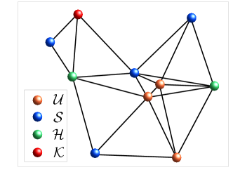
In our simulation, we consider a randomly generated connected network topology. There are a total of $N=10$ nodes in the network, and nodes are assumed connected when they are close enough geographically. The cardinalities of the subsets $\mathcal{U}$, $\mathcal{S}$, $\mathcal{H}$ and $\mathcal{K}$ are set to be $3$, $4$, $2$ and $1$, respectively. The nodes are partitioned into these four subsets randomly. The dimension of the decision vector is $M=5$. The random vectors $\bm{u}_{k,i}$ and $\bm{s}_{k,i}$ are generated according to the Gaussian distributions $\mathcal{N}(\mathds{1},I_{M})$ and $\mathcal{N}(0,I_{M})$, respectively. We set $b_{0}=5$ and the parameters $\{h_{k},b_{k}\}$ for $k\in\mathcal{H}$ to

$$h_{k_{1}}=\left[1\;2\;\cdots\;5\right],\quad b_{k_{1}}=2$$ (117)

$$h_{k_{2}}=\left[5\;4\;\cdots\;1\right],\quad b_{k_{2}}=3$$ (118)

where $k_{1}$ and $k_{2}$ are the indices of the two nodes in the subset $\mathcal{H}$. Furthermore, we use the barrier function given by (15) in [3] in our simulation with $t=10$, $\rho=0.1$ and $\tau=0.1$. We set the combination coefficients $\{a_{lk}\}$ to the Metropolis rule (See Table III in [23]) for both ATC and CTA strategies. The weights $\{c_{lk}\}$ are set to $c_{lk}=1$ for $l=k$ and zero otherwise, i.e., there is no exchange of gradient information among neighbors. According to Theorem 3, such a choice will always guarantee condition (84) so that the bias can be made arbitrarily small for small step-sizes. In our simulation, we do not assume the statistics of $\{\bm{u}_{k,i}\}$ and $\{\bm{s}_{k,i}\}$ are known to the nodes. The only information available is their realizations and the algorithms have to learn the best decision vector $w$ from them. Therefore, we use the following stochastic gradient vector at each node $k$:

$$\widehat{\nabla_{w}J_{k}}(w) =\begin{cases}-\bm{u}_{k,i}+\sum_{m=1}^{M}\nabla_{w}\phi(-e_{m}^{T}w)&k\in\mathcal{U}\\ 2\bm{s}_{k,i}+\sum_{m=1}^{M}\nabla_{w}\phi(-e_{m}^{T}w)&k\in\mathcal{S}\\ \nabla_{w}\phi(b_{k}-h_{k}^{T}w)+\sum_{m=1}^{M}\nabla_{w}\phi(-e_{m}^{T}w)&k\in\mathcal{H}\\ \nabla_{w}\phi(\mathds{1}^{T}w-b_{0})+\sum_{m=1}^{M}\nabla_{w}\phi(-e_{m}^{T}w)&k\in\mathcal{K}\end{cases}$$ (119)

To compare the performance with other algorithms, we also simulate the consensus-based approach from [16] with the same stochastic gradient as (119). The algorithm is listed below:

$$\bm{w}_{k,i}=\sum_{l\in\mathcal{N}_{k}}a_{lk}\bm{w}_{l,i-1}-\mu\widehat{\nabla_{w}J_{k}}(\bm{w}_{k,i-1})$$ (120)

Furthermore, we also simulate the conventional centralized approach to such optimization problem, which collects data from all nodes and implements stochstic gradient descent at the central node:

$$\bm{w}_{i}=\bm{w}_{i-1}-\mu\frac{1}{N}\sum_{k=1}^{N}\widehat{\nabla_{w}J_{k}}(\bm{w}_{i-1})$$ (121)

where the factor of $1/N$ is used to make the convergence rate the same as the distributed algorithms.

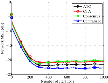
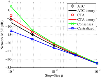
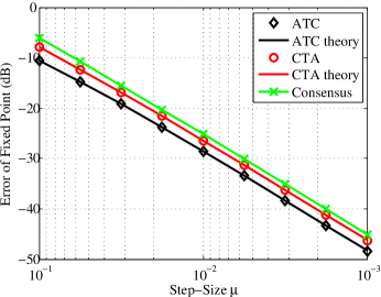
The simulatin results are shown in Fig. 4(a)–4(d). Fig. 4(a) shows the network topology, and Fig. 4(b) shows the learning curves of different algorithms. We see that ATC outperforms CTA and CTA outperforms consensus. To further compare the steady-state performance, we plot the steady-state MSE for different values of step-sizes in Fig. 4(c). We also plot the theoretical curves from (109)–(110) for ATC and CTA algorithms. We observe that all algorithms approach the performance of the centralized solution when the step-sizes are small. However, diffusion algorithms always outperform the consensus-based strategy; the gap between ATC and consensus algorithm is about $8$ dB when $\mu=0.1$. We also see that the theoretical curves match the simulated ones well. Finally, we recall that Theorem 3 shows that the error between the fixed point $w_{\infty}$ and $\mathds{1}\otimes w^{o}$ can be made arbitrarily small for small step-sizes, and the error $\|w_{\infty}-\mathds{1}\otimes w^{o}\|^{2}$ is on the order of $O(\mu^{2})$. To illustrate the result, we simulate the algorithms using true gradients $\{\nabla_{w}J_{k}(w)\}$ so that they converge to their fixed point $w_{\infty}$, and we get different values of $w_{\infty}$ for different step-sizes. The theoretical values for ATC and CTA can be computed from (83). The results are shown in Fig. 4(d). We see that the theory matches simulation, and the power of the fixed point error per node decays at $20$dB per decade, which is $O(\mu^{2})$ and is consistent with (85). Note that diffusion algorithms outperform the consensus. Also note from (83) and (100) that the bias and the fixed point error have the same expression. Therefore, diffusion algorithms have smaller bias than consensus (the gap in Fig. 4(d) is as large as $5$dB between ATC and consensus).

V Conclusion

This paper generalized diffusion adaptation strategies to perform multi-objective optimization in a distributed manner over a network of nodes. We use constant step-sizes to endow the network with continuous learning and adaptation abilities via local interactions. We analyzed the mean-square-error performance of the diffusion strategy, and showed that the solution at each node gets arbitrarily close to the same Pareto-optimal solution for small step-sizes.

Appendix A Properties of the Operators

Properties 1-3 are straightforward from the definitions of $T_{A}(\cdot)$ and $P[\cdot]$. We therefore omit the proof for brevity, and start with property 4.

(Property 4: Convexity)
We can express each $N\times 1$ block vector $x^{(k)}$ in the form $x^{(k)}=\mathrm{col}\{x_{1}^{(k)},\ldots,x_{N}^{(k)}\}$ for $k=1,\ldots,N$. Then, the convex combination of $x^{(1)},\ldots,x^{(N)}$ can be expressed as

$$\sum_{k=1}^{K}a_{l}\;x^{(k)}=\mathrm{col}\Big{\{}\sum_{k=1}^{K}a_{l}x_{1}^{(k)},\ldots,\sum_{k=1}^{K}a_{l}x_{N}^{(k)}\Big{\}}$$ (122)

According to the definition of the operator $P[\cdot]$, and in view of the convexity of $\|\cdot\|^{2}$, we have

$$P\Big{[}\sum_{k=1}^{K}a_{l}\;x^{(k)}\Big{]} =\mathrm{col}\Big{\{}\big{\|}\sum_{k=1}^{K}a_{l}x_{1}^{(k)}\big{\|}^{2},\ldots,\big{\|}\sum_{k=1}^{K}a_{l}x_{N}^{(k)}\big{\|}^{2}\Big{\}}$$

$$\preceq\mathrm{col}\Big{\{}\sum_{k=1}^{K}a_{l}\|x_{1}^{(k)}\|^{2},\ldots,\sum_{k=1}^{K}a_{l}\|x_{N}^{(k)}\|^{2}\Big{\}}$$

$$=\sum_{k=1}^{K}a_{l}\;P[x^{(k)}]$$ (123)

(Property 5: Additivity)
By the definition of $P[\cdot]$ and the assumption that $\mathbb{E}\bm{x}_{k}^{T}\bm{y}_{k}=0$ for each $k=1,\ldots,N$, we obtain

$$\mathbb{E}P[\bm{x}+\bm{y}] =\mathrm{col}\{\mathbb{E}\|\bm{x}_{1}+\bm{y}_{1}\|^{2},\;\ldots,\;\mathbb{E}\|\bm{x}_{N}+\bm{y}_{N}\|^{2}\}$$

$$=\mathrm{col}\{\mathbb{E}\|\bm{x}_{1}\|^{2}+\mathbb{E}\|\bm{y}_{1}\|^{2},\;\ldots,\;\mathbb{E}\|\bm{x}_{N}\|^{2}+\mathbb{E}\|\bm{y}_{N}\|^{2}\}$$

$$=\mathbb{E}P[\bm{x}]+\mathbb{E}P[\bm{y}]$$ (124)

(Property 6: Variance Relations)
We first prove (35). From the definition of $T_{A}(\cdot)$ in (22) and the definition of $P[\cdot]$ in (24), we express

$$P[T_{A}(x)] =\mathrm{col}\Big{\{}\big{\|}\sum_{l=1}^{N}a_{l1}x_{l}\big{\|}^{2},\;\ldots,\;\big{\|}\sum_{l=1}^{N}a_{lN}x_{l}\big{\|}^{2}\Big{\}}$$ (125)

Since $\|\cdot\|^{2}$ is a convex function and each sum inside the squared norm operator is a convex combination of $x_{1},\ldots,x_{N}$ ($A^{T}$ is right stochastic), by Jensen’s inequality[2, p.77], we have

$$P[T_{A}(x)] \preceq\mathrm{col}\Big{\{}\sum_{l=1}^{N}a_{l1}\|x_{l}\|^{2},\;\ldots,\;\sum_{l=1}^{N}a_{lN}\|x_{l}\|^{2}\Big{\}}$$

$$=A^{T}\mathrm{col}\{\|x_{1}\|^{2},\;\ldots,\;\|x_{N}\|^{2}\}$$

$$=A^{T}P[x]$$ (126)

Next, we proceed to prove (36). We need to call upon the following useful lemmas from [4, p.24], and Lemmas 1–2 in[21], respectively.

Lemma 4 (Mean-Value Theorem).

For any twice-differentiable function $f(\cdot)$, it holds that

$$\nabla f(y)=\nabla f(x)+\left[\int_{0}^{1}\nabla^{2}f\big{(}x+t(y-x)\big{)}dt\right](y-x)$$ (127)

where $\nabla^{2}f(\cdot)$ denotes the Hessian of $f(\cdot)$, and is a symmetric matrix. ∎

Lemma 5 (Bounds on the Integral of Hessian).

Under Assumption 1, the following bounds hold for any vectors ${x}$ and ${y}$:

$$\lambda_{l,\min}I_{M}\leq\int_{0}^{1}\nabla_{w}^{2}J_{l}({x}+t{y})dt\leq\lambda_{l,\max}I_{M}$$ (128)

$$\left\|I-\mu_{k}\sum_{l=1}^{N}c_{lk}\left[\int_{0}^{1}\nabla_{w}^{2}J_{l}({x}+t{y})dt\right]\right\|\leq\gamma_{k}$$ (129)

where $\|\cdot\|$ denotes the $2-$induced norm, and $\gamma_{k}$, $\sigma_{k,\min}$ and $\sigma_{k,\max}$ were defined in (38)–(39). ∎

By the definition of the operator $T_{G}(\cdot)$ in (23) and the expression (127), we express $T_{G}(x)-T_{G}(y)$ as

$$T_{G}(x)-T_{G}(y)= \begin{bmatrix}\displaystyle\left[I_{M}\!-\!\mu_{1}\sum_{l=1}^{N}c_{l1}\!\!\int_{0}^{1}\!\!\nabla_{w}^{2}J_{l}(y_{1}\!+\!t(x_{1}\!-\!y_{1}))dt\right]\!(x_{1}\!-\!y_{1})\\ \vdots\\ \displaystyle\left[I_{M}\!-\!\mu_{N}\sum_{l=1}^{N}c_{lN}\!\!\int_{0}^{1}\!\!\nabla_{w}^{2}J_{l}(y_{N}\!+\!t(x_{N}\!-\!y_{N}))dt\right]\!(x_{N}\!-\!y_{N})\end{bmatrix}$$ (130)

Therefore, using (129) and the definition of $P[\cdot]$ in (24), we obtain

$$P[T_{G}(x)-T_{G}(y)] \preceq\mathrm{col}\left\{\gamma_{1}^{2}\cdot\|x_{1}-y_{1}\|^{2},\ldots,\gamma_{N}^{2}\cdot\|x_{N}-y_{N}\|^{2}\right\}$$

$$=\Gamma^{2}P[x-y]$$ (131)

(Property 7: Block Maximum Norm)
According to the definition of $P[\cdot]$ and the definition of block maximum norm [21], we have

$$\|P[x]\|_{\infty} =\big{\|}\mathrm{col}\{\|x_{1}\|^{2},\;\ldots,\;\|x_{N}\|^{2}\}\big{\|}_{\infty}$$

$$=\max_{1\leq k\leq N}\|x_{k}\|^{2}$$

$$=\big{(}\max_{1\leq k\leq N}\|x_{k}\|\big{)}^{2}$$

$$=\|x\|_{b,\infty}^{2}$$ (132)

(Property 8: Preservation of Inequality)
To prove $Fx\preceq Fy$, it suffices to prove $0\preceq F(y-x)$. Since $x\preceq y$, we have $0\preceq y-x$, i.e., all entries of the vector $y-x$ are nonnegative. Furthermore, since all entries of the matrix $F$ are nonnegative, the entries of the vector $F(y-x)$ are all nonnegative, which means $0\preceq F(y-x)$.

Appendix B Bias at Small Step-Sizes

It suffices to show that

$$\lim_{\mu_{\max}\rightarrow 0}\frac{\|\mathds{1}\otimes w^{o}-w_{\infty}\|}{\mu_{\max}}=\xi$$ (133)

where $\xi$ is a constant independent of $\mu_{\max}$. It is known that any matrix is similar to a Jordan canonical form [36]. Hence, there exists an invertible matrix $Y$ such that $A_{2}^{T}A_{1}^{T}=YJY^{-1}$, where $J$ is the Jordan canonical form of the matrix $A_{2}^{T}A_{1}^{T}$, and the columns of the matrix $Y$ are the corresponding right principal vectors of various degrees [36, pp.82–88]; the right principal vector of degree one is the right eigenvector. Obviously, the matrices $J$ and $Y$ are independent of $\mu_{\max}$. Using the Kronecker product property[36, p.140]: $(A\otimes B)(C\otimes D)=AC\otimes BD$, we obtain

$$\mathcal{A}_{2}^{T}\mathcal{A}_{1}^{T} =A_{2}^{T}A_{1}^{T}\otimes I_{M}$$

$$=(Y\otimes I_{M})(J\otimes I_{M})(Y^{-1}\otimes I_{M})$$ (134)

Denote $\mu_{k}=\beta_{k}\mu_{\max}$, where $\beta_{k}$ is some positive scalar such that $0<\beta_{k}\leq 1$. Substituting (134) into (83), we obtain

$$\mathds{1}\otimes w^{o}-w_{\infty} =\left[I_{MN}-\mathcal{A}_{2}^{T}\mathcal{A}_{1}^{T}+\mathcal{A}_{2}^{T}\mathcal{M}{\mathcal{R}}_{\infty}\mathcal{A}_{1}^{T}\right]^{-1}\mathcal{A}_{2}^{T}\mathcal{M}\mathcal{C}^{T}g^{o}$$

$$=(Y\otimes I_{M})\left[I_{MN}-J\otimes I_{M}+\mu_{\max}E\right]^{-1}(Y^{-1}\otimes I_{M})\mathcal{A}_{2}^{T}\mathcal{M}\mathcal{C}^{T}g^{o}$$ (135)

where

$$E =(Y^{-1}\otimes I_{M})\mathcal{A}_{2}^{T}\mathcal{M}_{0}\mathcal{R}_{\infty}\mathcal{A}_{1}^{T}(Y\otimes I_{M})$$ (136)

$$\mathcal{M}_{0} \triangleq\mathcal{M}/\mu_{\max}=\underbrace{\mathrm{diag}\{\beta_{1},\ldots,\beta_{N}\}}_{\triangleq\Omega_{0}}\otimes I_{M}$$ (137)

By (8), the matrix $A_{2}^{T}A_{1}^{T}$ is right-stochastic, and since $A_{2}^{T}A_{1}^{T}$ is regular, it will have an eigenvalue of one that has multiplicity one and is strictly greater than all other eigenvalues[37]. Furthermore, the corresponding left and right eigenvectors are $\theta^{T}$ and $\mathds{1}$, with $\theta^{T}\succ 0$ (all entries of the row vector $\theta^{T}$ are real positive numbers). For this reason, we can partition $J$, $Y^{-1}$ and $Y$ in the following block forms:

$$J=\mathrm{diag}\{1,\;J_{0}\},\quad Y^{-1}=\mathrm{col}\left\{\frac{\theta^{T}}{\theta^{T}\mathds{1}},\;Y_{R}\right\},\quad Y=\left[\mathds{1}\;Y_{L}\right]$$ (138)

where $J_{0}$ is an $(N-1)\times(N-1)$ matrix that contains the Jordan blocks of eigenvalues strictly within unit circle, i.e., $\rho(J_{0})<1$. The first row of the matrix $Y^{-1}$ in (138) is normalized by $\theta^{T}\mathds{1}$ so that $Y^{-1}Y=I$. (Note that $Y^{-1}Y=I$ requires the product of the first row of $Y^{-1}$ and the first column of $Y$ to be one: $\frac{\theta^{T}}{\theta^{T}\mathds{1}}\mathds{1}=1$.) Substituting these partitionings into (136), we can express $E$ as

$$E =\begin{bmatrix}E_{11}&E_{12}\\ E_{21}&E_{22}\end{bmatrix}$$ (139)

where

$$E_{11} \triangleq\big{(}\frac{\theta^{T}}{\theta^{T}\mathds{1}}\otimes I_{M}\big{)}\mathcal{A}_{2}^{T}\mathcal{M}_{0}\mathcal{R}_{\infty}\mathcal{A}_{1}^{T}(\mathds{1}\otimes I_{M})$$ (140)

$$E_{12} \triangleq\big{(}\frac{\theta^{T}}{\theta^{T}\mathds{1}}\otimes I_{M}\big{)}\mathcal{A}_{2}^{T}\mathcal{M}_{0}\mathcal{R}_{\infty}\mathcal{A}_{1}^{T}(Y_{L}\otimes I_{M})$$ (141)

$$E_{21} \triangleq(Y_{R}\otimes I_{M})\mathcal{A}_{2}^{T}\mathcal{M}_{0}\mathcal{R}_{\infty}\mathcal{A}_{1}^{T}(\mathds{1}\otimes I_{M})$$ (142)

$$E_{22} \triangleq(Y_{R}\otimes I_{M})\mathcal{A}_{2}^{T}\mathcal{M}_{0}\mathcal{R}_{\infty}\mathcal{A}_{1}^{T}(Y_{L}\otimes I_{M})$$ (143)

Observe that the matrices $E_{11}$, $E_{12}$, $E_{21}$ and $E_{22}$ are independent of $\mu_{\max}$. Substituting (138) and (139) into (135), we obtain

$$\mathds{1}\otimes w^{o}\!-\!w_{\infty} =(Y\otimes I_{M})\begin{bmatrix}\mu_{\max}E_{11}&\mu_{\max}E_{12}\\ \mu_{\max}E_{21}&I\!-\!J_{0}\otimes I_{M}\!+\!\mu_{\max}E_{22}\end{bmatrix}^{-1}\begin{bmatrix}\frac{1}{\theta^{T}\mathds{1}}(\theta^{T}\otimes I_{M})\mathcal{A}_{2}^{T}\mathcal{M}\mathcal{C}^{T}g^{o}\\ (Y_{R}\otimes I_{M})\mathcal{A}_{2}^{T}\mathcal{M}\mathcal{C}^{T}g^{o}\end{bmatrix}$$ (144)

Let us denote

$$\begin{bmatrix}G_{11}&G_{12}\\ G_{21}&G_{22}\end{bmatrix}\triangleq\begin{bmatrix}\mu_{\max}E_{11}&\!\mu_{\max}E_{12}\\ \mu_{\max}E_{21}&\!I\!-\!J_{0}\otimes I_{M}\!+\!\mu_{\max}E_{22}\end{bmatrix}^{-1}$$ (145)

Furthermore, recalling that $w^{o}$ is the minimizer of the global cost function (4), we have

$$\sum_{l=1}^{N}\nabla_{w}J_{l}(w^{o})=0\quad\Leftrightarrow\quad(\mathds{1}^{T}\otimes I_{M})\;g^{o}=0$$ (146)

which, together with condition (84), implies that

$$(\theta^{T}\otimes I_{M})\mathcal{A}_{2}^{T}\mathcal{M}\mathcal{C}^{T}g^{o}= \;(\theta^{T}A_{2}^{T}\Omega C^{T}\otimes I_{M})g^{o}$$

$$= \;c_{0}(\mathds{1}^{T}\otimes I_{M})g^{o}$$

$$= \;0$$ (147)

where we also used the facts that $\mathcal{A}_{2}^{T}=A_{2}^{T}\otimes I_{M}$, $\mathcal{C}^{T}=C^{T}\otimes I_{M}$, $\mathcal{M}=\Omega\otimes I_{M}$ and the Kronecker product property: $(A\otimes B)(C\otimes D)$. Substituting (145) and (147) into (144) and using (137) lead to

$$\mathds{1}\otimes w^{o}-w_{\infty} =\mu_{\max}\cdot(Y\otimes I_{M})\!\begin{bmatrix}G_{12}\\ G_{22}\end{bmatrix}(Y_{R}A_{2}^{T}\Omega_{0}C^{T}\otimes I_{M})g^{o}$$ (148)

To proceed with analysis, we need to evaluate $G_{12}$ and $G_{22}$. We call upon the relation from [36, pp.48]:

$$\begin{bmatrix}P&Q\\ U&V\end{bmatrix}^{-1}=\begin{bmatrix}P^{-1}+P^{-1}QSUP^{-1}&-P^{-1}QS\\ -SUP^{-1}&S\end{bmatrix}$$ (149)

where $S=(V-UP^{-1}Q)^{-1}$. To apply the above relation to (145), we first need to verify that $E_{11}$ is invertible. By definition (140),

$$E_{11}= \;\big{(}\frac{\theta^{T}}{\theta^{T}\mathds{1}}A_{2}^{T}\Omega_{0}\otimes I_{M}\big{)}\mathcal{R}_{\infty}(A_{1}^{T}\mathds{1}\otimes I_{M})$$

$$= \;(z^{T}\otimes I_{M})\mathcal{R}_{\infty}(\mathds{1}\otimes I_{M})$$

$$= \;\sum_{k=1}^{N}z_{k}\sum_{l=1}^{N}c_{lk}H_{lk,\infty}$$ (150)

where $z_{k}$ denotes the $k$th entry of the vector $z\triangleq\Omega_{0}A_{2}\theta/\theta^{T}\mathds{1}$ (note that all entries of $z$ are non-negative, i.e., $z_{k}\geq 0$). Recall from (77) that $H_{lk,\infty}$ is a symmetric positive semi-definite matrix. Moreover, since $z_{k}$ and $c_{lk}$ are nonnegative, we can conclude from (150) that $E_{11}$ is a symmetric positive semi-definite matrix. Next, we show that $E_{11}$ is actually strictly positive definite. Applying (128) to the expression of $H_{lk,\infty}$ in (77), we obtain $H_{lk,\infty}\geq\lambda_{l,\min}I_{M}$. Substituting into (150) gives:

$$E_{11}\geq \;\left[\sum_{k=1}^{N}z_{k}\sum_{l=1}^{N}c_{lk}\lambda_{l,\min}\right]\cdot I_{M}$$

$$\geq \;\Big{(}\sum_{k=1}^{N}z_{k}\Big{)}\min_{1\leq k\leq N}\Big{\{}\sum_{l=1}^{N}c_{lk}\lambda_{l,\min}\Big{\}}\cdot I_{M}$$

$$= \;\frac{\mathds{1}^{T}\Omega_{0}A_{2}\theta}{\theta^{T}\mathds{1}}\cdot\min_{1\leq k\leq N}\Big{\{}\sum_{l=1}^{N}c_{lk}\lambda_{l,\min}\Big{\}}\cdot I_{M}$$ (151)

Noting that the matrices $\Omega_{0}$ and $A_{0}$ have nonnegative entries with some entries being positive, and that all entries of $\theta$ are positive, we have $({\mathds{1}^{T}\Omega_{0}A_{2}\theta})/({\theta^{T}\mathds{1}})>0$. Furthermore, by Assumption 1, we know $\sum_{l=1}^{N}c_{lk}\lambda_{l,\min}>0$ for each $k=1,\ldots,N$. Therefore, we conclude that $E_{11}>0$ and is invertible. Applying (149) to (145), we get

$$G_{12} =-E_{11}^{-1}E_{12}G_{22}$$ (152)

$$G_{22} =\left[I\!-\!J_{0}\otimes I_{M}\!+\!\mu_{\max}(E_{22}\!-\!E_{21}E_{11}^{-1}E_{12}^{T})\right]^{-1}$$ (153)

Substituting (153) into (148) leads to

$$\mathds{1}\otimes w^{o}-w_{\infty}= \;\mu_{\max}\cdot(Y\otimes I_{M})\!\begin{bmatrix}-E_{11}^{-1}E_{12}\\ I\end{bmatrix}G_{22}(Y_{R}A_{2}^{T}\Omega_{0}C^{T}\otimes I_{M})g^{o}$$ (154)

Substituting expression (154) into the left-hand side of (133), we get

$$\lim_{\mu_{\max}\rightarrow 0}\frac{\|\mathds{1}\otimes w^{o}-w_{\infty}\|}{\mu_{\max}} =\!\!\!\lim_{\mu_{\max}\rightarrow 0}\bigg{\|}(Y\otimes I_{M})\!\begin{bmatrix}-E_{11}^{-1}E_{12}\\ I\end{bmatrix}G_{22}(Y_{R}A_{2}^{T}\Omega_{0}C^{T}\otimes I_{M})g^{o}\bigg{\|}$$ (155)

Observe that the only term on the right-hand side of (155) that depends on $\mu_{\max}$ is $G_{22}$. From its expression (153), we observe that, as $\mu_{\max}\rightarrow 0$, the matrix $G_{22}$ tends to $(I-J_{0}\otimes I_{M})^{-1}$, which is independent of $\mu_{\max}$. Therefore, the limit on the right-hand side of (155) is independent of $\mu_{\max}$.

References

- [1] J. Chen and A. H. Sayed, “Distributed Pareto-optimal solutions via diffusion adaptation,” in Proc. IEEE Workshop on Statistical Signal Process. (SSP), Ann Arbor, MI, Aug. 2012, pp. 1–4.
- [2] S. P. Boyd and L. Vandenberghe, Convex Optimization, Cambridge University Press, 2004.
- [3] Z. J. Towfic, J. Chen, and A. H. Sayed, “Distributed throughput optimization over P2P mesh networks using diffusion adaptation,” in Proc. IEEE International Conf. Commun. (ICC), Ottawa, Canada, June 2012, pp. 1–5.
- [4] B. Polyak, Introduction to Optimization, Optimization Software, NY, 1987.
- [5] D.P. Bertsekas and J.N. Tsitsiklis, Parallel and Distributed Computation: Numerical Methods, Athena Scientific, Belmont, 1997.
- [6] D. P. Bertsekas, “A new class of incremental gradient methods for least squares problems,” SIAM J. Optim., vol. 7, no. 4, pp. 913–926, 1997.
- [7] A. Nedic and D. P. Bertsekas, “Incremental subgradient methods for nondifferentiable optimization,” SIAM J. Optim., vol. 12, no. 1, pp. 109–138, 2001.
- [8] A. Nedic and D. P. Bertsekas, “Convergence rate of incremental subgradient algorithms,” Stochastic Optimization: Algorithms and Applications, S. Uryasev and P. M. Pardalos, Eds., pp. 263–304, 2000.
- [9] B. T. Polyak and Y. Z. Tsypkin, “Pseudogradient adaptation and training algorithms,” Automation and Remote Control, vol. 12, pp. 83–94, 1973.
- [10] M. G. Rabbat and R. D. Nowak, “Quantized incremental algorithms for distributed optimization,” IEEE J. Sel. Areas Commun., vol. 23, no. 4, pp. 798–808, 2005.
- [11] C. G. Lopes and A. H. Sayed, “Incremental adaptive strategies over distributed networks,” IEEE Trans. Signal Process., vol. 55, no. 8, pp. 4064–4077, Aug. 2007.
- [12] L. Li and J. A. Chambers, “A new incremental affine projection-based adaptive algorithm for distributed networks,” Signal Processing, vol. 88, no. 10, pp. 2599–2603, Oct. 2008.
- [13] R. M. Karp, “Reducibility among combinational problems,” Complexity of Computer Computations, R. E. Miller and J. W. Thatcher, Eds., pp. 85–104, 1972.
- [14] J. N. Tsitsiklis, D. P. Bertsekas, and M. Athans, “Distributed asynchronous deterministic and stochastic gradient optimization algorithms,” IEEE Trans. Autom. Control, vol. 31, no. 9, pp. 803–812, 1986.
- [15] S. Barbarossa and G. Scutari, “Bio-inspired sensor network design,” IEEE Signal Process. Mag., vol. 24, no. 3, pp. 26–35, 2007.
- [16] A. Nedic and A. Ozdaglar, “Distributed subgradient methods for multi-agent optimization,” IEEE Trans. Autom. Control, vol. 54, no. 1, pp. 48–61, 2009.
- [17] S. Kar and J. M. F. Moura, “Convergence rate analysis of distributed gossip (linear parameter) estimation: Fundamental limits and tradeoffs,” IEEE J. Sel. Topics. Signal Process., vol. 5, no. 4, pp. 674–690, Aug. 2011.
- [18] A. G. Dimakis, S. Kar, J. M. F. Moura, M. G. Rabbat, and A. Scaglione, “Gossip algorithms for distributed signal processing,” Proc. IEEE, vol. 98, no. 11, pp. 1847–1864, 2010.
- [19] K. Srivastava and A. Nedic, “Distributed asynchronous constrained stochastic optimization,” IEEE J. Sel. Topics Signal Process., vol. 5, no. 4, pp. 772–790, Aug. 2011.
- [20] U. A. Khan and A. Jadbabaie, “Networked estimation under information constraints,” Arxiv preprint arXiv:1111.4580, Nov. 2011.
- [21] J. Chen and A. H. Sayed, “Diffusion adaptation strategies for distributed optimization and learning over networks,” IEEE Trans. Signal Process., vol. 60, no. 8, pp. 4289–4305, Aug. 2012.
- [22] C. G. Lopes and A. H. Sayed, “Diffusion least-mean squares over adaptive networks: Formulation and performance analysis,” IEEE Trans. Signal Process., vol. 56, no. 7, pp. 3122–3136, July 2008.
- [23] F. S. Cattivelli and A. H. Sayed, “Diffusion LMS strategies for distributed estimation,” IEEE Trans. Signal Process., vol. 58, no. 3, pp. 1035–1048, March 2010.
- [24] S. S. Ram, A. Nedic, and V. V. Veeravalli, “Distributed stochastic subgradient projection algorithms for convex optimization,” J. Optim. Theory Appl., vol. 147, no. 3, pp. 516–545, 2010.
- [25] S.-Y. Tu and A. H. Sayed, “Mobile adaptive networks,” IEEE J. Sel. Topics. Signal Process., vol. 5, no. 4, pp. 649–664, Aug. 2011.
- [26] P. Di Lorenzo and S. Barbarossa, “A bio-inspired swarming algorithm for decentralized access in cognitive radio,” IEEE Trans. Signal Process., vol. 59, no. 12, pp. 6160–6174, Dec. 2011.
- [27] S. Chouvardas, K. Slavakis, and S. Theodoridis, “Adaptive robust distributed learning in diffusion sensor networks,” IEEE Trans. Signal Process., vol. 59, no. 10, pp. 4692–4707, Oct. 2011.
- [28] S. Theodoridis, K. Slavakis, and I. Yamada, “Adaptive learning in a world of projections,” IEEE Signal Process. Mag., vol. 28, no. 1, pp. 97–123, Jan. 2011.
- [29] E. Kreyszig, Introductory Functional Analysis with Applications, Wiley, NY, 1989.
- [30] N. Takahashi and I. Yamada, “Link probability control for probabilistic diffusion least-mean squares over resource-constrained networks,” in IEEE ICASSP, Dallas, TX, Mar. 2010, pp. 3518–3521.
- [31] A. H. Sayed, Adaptive Filters, Wiley, NJ, 2008.
- [32] H. Markowitz, “Portfolio selection,” The Journal of Finance, vol. 7, no. 1, pp. 77–91, 1952.
- [33] M. Rubinstein, “Markowitz’s “Portfolio Selection”: A Fifty-Year Retrospective,” The Journal of Finance, vol. 57, no. 3, pp. 1041–1045, Jun. 2002.
- [34] A. D. Fitt, “Markowitz portfolio theory for soccer spread betting,” IMA Journal of Management Mathematics, vol. 20, no. 2, pp. 167–184, Apr. 2009.
- [35] E. J. Elton, M. J. Gruber, and C. R. Blake, “Applications of Markowitz portfolio theory to pension fund design,” in Handbook of Portfolio Construction, J. B. Guerard, Ed., pp. 419–438. Springer, US, 2010.
- [36] A. J. Laub, Matrix Analysis for Scientists and Engineers, SIAM, PA, 2005.
- [37] R. A. Horn and C. R. Johnson, Matrix Analysis, Cambridge University Press, 1990.