Radiation matter entanglement

Abstract

The quantization of the electromagnetic field in the presence of material bodies, at zero temperature is considered. It is shown that a dielectric does not act as thermal bath for the field and yields a non-trivial non-thermal mixed state of the field. The properties of this state and its entropy are studied. The dependence of the second Renyi entropy of the field on the distance between dispersive objects is shown to decay as $R^{-4}$ for generic bodies.

I Introduction

The study of quantum correlations and entanglement in many body quantum systems has become a major theme in recent years. In particular, many-body systems are studied in terms of the reduced density matrices describing the state of constituents of the system. This point of view gives rise to various questions such as the question of thermalization: When can a part of a quantum system be considered as effectively in a thermal state?

Naturally, thermal density matrices appear in systems weakly coupled to a thermal heat bath. Moreover, it has recently been argued that a canonical thermal state may arise for typical pure states of the system+bath Hilbert space after tracing out the bath Goldstein et al. (2006); Popescu et al. (2006). However, many physical systems of interest are not typical and violate some of the assumptions leading to thermalization. In particular, the system considered here, that of a boson radiation field interacting with a dielectric medium, characterized by a dielectric function $\varepsilon(\omega)$, has been shown Klich (2012) to be described by a density matrix which is not thermal for the typical frequency dependence of the dielectric function $\varepsilon(\omega)$.

The dielectric function serves as a convenient way to encode the particular long wavelength properties of the material Lifshitz and Pitaevskii (1984). The dielectric susceptibility of the material, and it’s relations with various response functions serves to define an effective action for the field, and through it enables one to describe the actual state of it.

In this paper we continue the investigation, initiated in Klich (2012) of the reduced density matrix of a boson field in contact with a dispersive medium. Such a field may describe many other situations, such as phonons in a solid. The resulting photonic density matrix, of a field interacting with realistic materials, is in general not in a pure state and should be described in terms of a mixed state density matrix. This situation is in stark contrast to idealized Dirichlet or Neumann boundaries, which are consistent with a field Hamiltonian. The main observation is that the resulting mixed state of the field is not thermal, which may be a consequence of the nature of the model we consider, which is, in essence, integrable, and thus not typical.

As a measure of the field-matter entanglement, we use the entanglement entropy of the field. The entropy of radiation coupled to matter has been considered in numerous works. However, usually, the focus is on a single degree of freedom coupled to a bath of oscillators: For example, the entropy of a spin in the spin-boson model within the frame work of the Caldeira-Legget model Caldeira and Leggett (1981) was considered in Le Hur (2008) and the entanglement of a single radiation mode with an array of spins was studied in Lambert et al. (2004) for the Dicke model . The entanglement between spatially separated intervals of vacuum (or ground state of a spin chains) has been considered in Marcovitch et al. (2009); Calabrese et al. (2009). Here we have a system distinct from these works, and more akin to situations studied in macroscopic electrodynamic effects such as the Casimir and Van der Waals interactions between dielectric bodies.

Upon considering the entanglement entropy of the radiation field in contact with a material, it becomes clear that the entropy suffers from a UV divergence, and is thus explicitly cutoff dependent. Instead, in order to look for universal long-range features, we consider the distance dependent part of the second Renyi entropy of a field interacting with two distinct bodies. The second Renyi entanglement entropy is substantially more tractable analytically the full Von-Neumann entropy, but often contains the correct scaling behavior. Recently, Renyi entanglement entropies have been computed for numerous systems. For example, the ability to numerically access ${\cal S}_{2}$ has been used to probe entropy and topological entropy in recent works Hastings et al. (2010); Song et al. (2011); Ju et al. (2012).

In particular, we estimate the second Renyi entropy and find that:

$${\cal S}_{2}(A\cup B)-{\cal S}_{2}(A)-{\cal S}_{2}(B)=$$

$$-\omega_{{pA}}^{2}\omega_{{pB}}^{2}V_{A}V_{B}\frac{2\pi^{4}}{\omega_{0}^{2}R^{4}}+O({1\over R^{6}}),$$ (1)

where ${\cal S}_{2}(A)=-\log{\rm Tr}\rho_{\phi,A}^{2}.$ Here $\rho_{\phi,A}$ is the density matrix of a field in contact with a body $A$, after the body degrees of freedom have been integrated out. This result is of interest, as it shows that the decay of entanglement in this model is very slow compared to typical power laws in quantum electrodynamics such as interaction energies between dielectric bodies in the Casimir-Polder regime and compared to the toy-model studied in Klich (2012).

The paper is organized as follows. After a brief introduction of the problem, we proceed to review the description of density matrices of Gaussian states and their entropy. We then use this formalism to describe the state of a field in material medium using the equal time correlations of the field and field momenta operators. In the following section, we turn to the description of the distance dependent part of the entropy of a field interacting with two objects. We derive a formal expression for this entropy. Finally, we study the distance dependence of the second Renyi entropy obtaining the result (I).

II Gaussian effective action

The basic principles for describing field fluctuations in the vicinity of heated bodies have been comprehensively explored since the early days of electrodynamics (see e.g. Lifshitz and Pitaevskii (1984); Levin and Rytov (1967)). Within this approach, the macroscopic field interaction with the material is described through the dielectric response function $\varepsilon({\omega},{\bf x})$. Following this logic, here we study a simplified scalar field version of the electromagnetic field action

$$S={1\over 4\pi}\int{\rm d}^{3}x{{\rm d}\omega}\phi_{\omega}^{*}({\bf x})[{\omega}^{2}\varepsilon({\omega},{\bf x})-\nabla^{2}]\phi_{\omega}({\bf x}).$$ (2)

Throughout the paper we will also use the susceptibility $\chi$, which is related to the dielectric function $\varepsilon$ by $\varepsilon({\omega},{\bf x})=1+\chi(\omega,{\bf x})$.

When the permittivity is independent of $\omega$, the action is local in time, and one can easily quantize the associated scalar action assuming the conjugate momentum $\pi_{\phi}$ can be expressed in terms of $\dot{\phi}$ and doesn’t depend on external fields. Such an action follows from the Hamiltonian $H={1\over 4\pi}\int{\rm d}^{3}x[{\pi^{2}\over\varepsilon({\bf x})}+(\nabla\phi)^{2}]$. It describes, at zero temperature, a pure state, and as such will have no entropy. Note that $x$ dependence of $\varepsilon$ does not interfere with this property: it just means that the field has a spatially non-uniform mass, but can still be describe in terms of a Hamiltonian.

The situation is fundamentally different if $\varepsilon$ is $\omega$ dependent. The non-locality of the action (2) in time signals that our system is coupled to external degrees of freedom which have been integrated out, yielding a non trivial temporal response kernel. In such a case, the system cannot be in a pure state even at zero temperature, implying that our radiation field is entangled with the matter fields.

The effective action (2) can be obtained from integrating out other fields. To keep in mind a simple model for such a procedure we have in mind a bosonic field $\phi$ coupled with a matter field $\psi$. We consider the following typical action:

$$S_{\text{pure}}=\frac{1}{2}\int_{-\infty}^{\infty}{dt}\Big{\{}\int d^{3}x[\phi\left(-\partial_{t}^{2}+\nabla^{2}\right)\phi]+$$

$$\int_{B}d^{3}x[\frac{1}{8\pi^{2}}\psi\left(-\partial_{t}^{2}-\omega_{0}{}^{2}\right)\psi_{\omega}+\omega_{p}\psi(\partial_{t}\phi)]\Big{\}}$$ (3)

The action (II) corresponds to the form $\chi(\omega)=\frac{\omega_{p}{}^{2}}{\omega_{0}{}^{2}-\omega^{2}}$ of the response of $\phi$ to a transparent, but dispersive medium.

Dissipation may be introduced in a similar way, but requires coupling to an infinite bath of oscillators for each field degree of freedom, as done, e.g. in the Caldeira-Legget model Caldeira and Leggett (1981).

When quantizing a system starting from an effective action such as (2) it is important to keep in mind the following subtle point: the quantization procedure cannot be complete without additional information on the system. In our case, we will need the conjugate momentum operators to the field and their correlations. It is impossible to obtain those from the effective action alone. The reason is that while the action gives us full information about the field correlators, it does not define uniquely the momentum correlations: The momentum correlations are extracted from the time dependence of the field correlations through equations of motion, but these depend on the particular way the field is coupled to the matter.

To illustrate this point, we show that there may be some ambiguity on how to correctly choose those. For example, the terms $\phi\partial_{t}\psi$ and $-\psi\partial_{t}\phi$ in a field Lagrangian, while classically the same, as they are related by a full time derivatives, yield the same effective action for $\phi$ upon integrating $\psi$ out but, are not quantized in the same way. Indeed, let us look at the following simple example. Consider the two Lagraniangs:

$$L_{1}=\frac{1}{2}\left(\dot{\phi}^{2}-\omega_{0}{}^{2}\phi^{2}\right)+\frac{1}{2}\dot{\psi}^{2}-B\psi^{2}+a\dot{\psi}\phi$$ (4)

and

$$L_{2}=\frac{1}{2}\left(\dot{\phi}^{2}-\omega_{0}{}^{2}\phi^{2}\right)+\frac{1}{2}\dot{\psi}^{2}-B\psi^{2}-a\dot{\phi}\psi$$ (5)

which differ by a total derivative: $L_{1}-L_{2}=a\frac{d}{\text{dt}}({\phi\psi})$. Let us check, that when canonically quantizing them we get different Hamiltonians: From the Lagrangian $L_{1}$, we get the canonical: $P_{\phi}=\dot{\phi}$ and $P_{\psi}=\dot{\psi}+a\phi$ While $L_{2}$ gives us: $P_{\phi}=\dot{\phi}-a$ and $P_{\psi}=\dot{\psi}$.

Clearly, the time dependent correlation functions $\langle\phi(t)\phi(t^{\prime})\rangle$ computable from the action (2), will yield different results for $\langle\pi_{\phi}(t)\pi_{\phi}(t^{\prime})\rangle$ when computed from the equation of motion obtained from of the full Lagrangians $L_{1}$ and $L_{2}$.

In this paper we proceed choosing $\pi_{\phi}=\dot{\phi}$ motivated by the usual lagrangian coupling the electromagnetic field $A$ with material fields through $A\cdot J$.

III Gaussian states and their entropy

For a general many-body density matrix, determination of the state requires, in principle, the knowledge of all matrix elements of the density matrix. These scale exponentially with the number of degrees of freedom and for interacting systems become intractable very quickly. However, fortunately, for states described by Gaussian field theories the situation is considerably simpler. Indeed, by virtue of Wick’s theorem, all correlation functions, and thus all matrix elements can be obtained from the two point functions of the field. Thus, our task is to use the two point functions in order to represent the general state of the field. To proceed, in this section we review the method of calculating entropies of Gaussian states (see, e.g. Botero and Reznik (2003); Plenio and Virmani (2007)) from correlation functions. The material is standard, but for convenience, we choose review it here in detail.

Consider a scalar field with $n$ degrees of freedom $\phi_{n}$ and conjugate momenta $\pi_{n}=-i\partial_{\phi_{n}}$. It is convenient to bunch these together, defining the vector:

$$(O_{1},..O_{2n})=(\phi_{1},..\phi_{n},\pi_{1},..\pi_{n}).$$ (6)

Using this vector, the canonical commutation relations $[\phi_{n},\pi_{m}]=i\delta_{nm}$ may be expressed as:

$$[O_{j},O_{k}]=i\sigma_{j,k}$$ (7)

where $\sigma$ is the $2n\times 2n$ block matrix

$$\sigma=\left(\begin{array}[]{cc}0&I_{n}\\ -I_{n}&0\end{array}\right)$$ (10)

and we set $\hbar=1$ for convenience.

The commutation relations (7) as well as the hermiticity of the canonical field and momenta operators are preserved under the group of symplectic transformations $Sp(2n)$, the set of real matrices $W$ such that $W\sigma W^{T}=\sigma$.

As mentioned above, we would like to use the two point functions of the field to determine it’s state. To do this, let us first define the the covariance matrix:

$$\gamma_{jk}=2Re\langle(O_{j}-\langle O_{j}\rangle)(O_{k}-\langle O_{k}\rangle)\rangle.$$ (11)

The operators $O_{i}$ can always be redefined so that $\langle O_{j}\rangle=0$. In the rest of the paper we will assume our Gaussian field and field momenta have been correctly defined to have this property.

Next, we bring $\gamma$ into the canonical Williamson normal form:

$$W\gamma W^{T}=\left(\begin{array}[]{cc}{\tilde{\mu}}&0\\ 0&{\tilde{\mu}}\end{array}\right)\equiv M$$ (14)

Where ${\tilde{\mu}}$ is a diagonal matrix ${\tilde{\mu}}=diag(\mu_{1},...\mu_{n})$ and $W\in Sp(2n)$ . The $\mu_{i}$ are called the “symplectic eigenvalues” of $\gamma$, and they are equal to the positive eigenvalues of $i\sigma\gamma$.

To see this last property, let us check that if $i\sigma\gamma\psi=\mu\psi$ then $\mu^{2}$ is an eigenvalue of $M^{2}$. To see this one can explicitly check that $\sigma M\sigma M=-M^{2}$, therefore:

$$M^{2}=-\sigma M\sigma M=-\sigma W\gamma W^{T}\sigma W\gamma W^{T}=$$

$$-W^{-T}W^{T}\sigma W\gamma\sigma\gamma W^{T}=-W^{-T}\sigma\gamma\sigma\gamma W^{T}.$$

We conclude that

$$M^{2}(W^{-T}\psi)=W^{-T}(i\sigma\gamma)^{2}W^{T}W^{-T}\psi=\mu^{2}(W^{-T}\psi).$$ (15)

An additional, technical simplification, occurs, if we assume that no $\langle\phi\pi\rangle$ correlations are present, i.e. $\langle\phi\pi\rangle=0$. In this case the symplectic eigenvalues are equal to square roots of eigenvalues of ${\cal G}{\cal H}$, where ${\cal G}$ and ${\cal H}$ are field and field momentum two point functions, respectively. To see this property, consider a $\gamma$ which is block diagonal of the form:

$$\gamma=2\left(\begin{array}[]{cc}{\cal G}&0\\ 0&{\cal H}\end{array}\right)$$ (18)

Assume that $i\sigma\gamma\psi=\mu\psi$. It follows that $\gamma^{2}\psi=\mu^{2}\psi$. Computing, explicitly,

$$(i\sigma\gamma)^{2}=4\left(\begin{array}[]{cc}{\cal H}{\cal G}&0\\ 0&{\cal G}{\cal H}\end{array}\right)$$ (21)

Thus

$$(i\sigma\gamma)^{2}\left(\begin{array}[]{c}\psi_{1}\\ \psi_{2}\end{array}\right)=4\left(\begin{array}[]{c}{\cal H}{\cal G}\psi_{1}\\ {\cal G}{\cal H}\psi_{2}\end{array}\right)=4\mu^{2}\left(\begin{array}[]{c}\psi_{1}\\ \psi_{2}\end{array}\right)$$ (28)

and we conclude that $\mu^{2}$ is an eigenvalue of ${\cal G}{\cal H}$ (and, equivalently, of ${\cal H}{\cal G}$).

Next, we find the Gaussian state associated with the covariance matrix $\gamma$ by comparing to the covariance matrix of a general quadratic Hamiltonian in a thermal state.

Consider a quadratic Hamiltonian for coordinate and momenta $\phi,\pi$

$$H=\psi^{T}M\psi~{}~{}~{}~{}~{}~{};~{}~{}~{}~{}~{}\psi=\left(\begin{array}[]{c}\phi\\ \pi\end{array}\right),$$ (31)

where M is symmetric and real. We find the normal form

$$S^{T}MS=\left(\begin{array}[]{cc}{\Lambda}&0\\ 0&{\Lambda}\end{array}\right)$$ (34)

and let: $\psi=S\tilde{\psi}$. Then

$$H=\tilde{\psi}^{T}\left(\begin{array}[]{cc}{\Lambda}&0\\ 0&{\Lambda}\end{array}\right)\tilde{\psi}$$ (37)

In terms of the components $\tilde{\phi}_{i},\tilde{\pi}_{i}$ of $\tilde{\psi}$, the Hamiltonian breaks into independent oscillators of the form:

$$H=\Sigma_{i}H_{i}\text{ };\text{ }$$

$$H_{i}=\Lambda_{i}\left(\tilde{\phi}_{i}{}^{2}+\tilde{\pi}_{i}{}^{2}\right)=2\Lambda_{i}\left(a_{i}^{+}a_{i}+\frac{1}{2}\right)$$ (38)

where $a_{i}^{+}=\frac{1}{\sqrt{2}}\left(\tilde{\phi}_{i}-i\tilde{\pi}_{i}\right)$ are canonical bosonic creation operators.

Let us compute the finite temperature expectation values of $\tilde{\phi}_{i},\tilde{\pi}_{i}$. At an inverse finite temperature $\beta$ we have:

$$\left\langle\tilde{\phi}_{i}^{2}\right\rangle=\frac{1}{2}\left\langle\left(\tilde{a}_{i}{}^{+}+\tilde{a}_{i}\right){}^{2}\right\rangle=$$

$$\frac{1}{2}\left\langle 2\tilde{a}_{i}{}^{+}\tilde{a}_{i}+1\right\rangle=\tilde{n}_{i}+\frac{1}{2}=\frac{1}{e^{2\beta\Lambda_{i}}-1}+\frac{1}{2}$$ (39)

where $\tilde{n}_{i}=\tilde{a}_{i}{}^{+}\tilde{a}_{i}$ is the number occupation of mode $i$. Thus:

$$\tilde{\gamma}=2\left(\begin{array}[]{cc}\left\langle\tilde{\phi}_{i}\tilde{\phi}_{j}\right\rangle&\left\langle\tilde{\phi}_{i}\tilde{\pi}_{j}\right\rangle\\ \left\langle\tilde{\pi}_{i}\tilde{\phi}_{j}\right\rangle&\left\langle\tilde{\pi}_{i}\tilde{\pi}_{j}\right\rangle\end{array}\right)=2\left(\begin{array}[]{cc}\frac{1}{e^{2\beta{\Lambda}}-1}+\frac{1}{2}&0\\ 0&\frac{1}{e^{2\beta{\Lambda}}-1}+\frac{1}{2}\end{array}\right)$$

Finally, we rotate to the original basis, so that

$$\gamma=2\left(\begin{array}[]{cc}\left\langle\phi_{i}\phi_{j}\right\rangle&\left\langle\phi_{i}\pi_{j}\right\rangle\\ \left\langle\pi_{i}\phi_{j}\right\rangle&\left\langle\pi_{i}\pi_{j}\right\rangle\end{array}\right)=$$ (43)

$$2\left(S^{T}\right)^{-1}\left(\begin{array}[]{cc}\frac{1}{e^{2\beta{{\Lambda}}}-1}+\frac{1}{2}&0\\ 0&\frac{1}{e^{2\beta{\Lambda}}-1}+\frac{1}{2}\end{array}\right)S^{-1}.$$ (46)

Comparing (14) with (43), and setting $\beta=1$ we see that:

$${\mu_{i}\over 2}=\frac{1}{e^{2\Lambda_{i}}-1}+\frac{1}{2}.$$

Note that the choice of $\beta$ is arbitrary, since one can always rescale simultaneously $\beta$ and $\Lambda$ while keeping their product constant. Inverting the relation we find $e^{2\Lambda_{\text{eff}}}-1=2(\mu_{i}-1)^{-1}$, and finally:

$$2\Lambda_{i}=\log\frac{\mu_{i}+1}{\mu_{i}-1}.$$ (47)

Thus, we conclude that given a covariance matrix $\gamma$, and assuming this is a Gaussian state, then we can describe the state of the system as:

$$\rho=Z^{-1}e^{-\sum_{i}2\Lambda_{i}{a^{+}}_{i}a_{i}}~{};~{}2\Lambda_{i}=\log{\mu_{i}+1\over\mu_{i}-1}.$$ (48)

Next, let us compute the entropy of this state in terms of the symplectic eigenvalues $\mu_{i}$. Since the density matrix factors into independent modes, we may consider first a single $i$ mode. For a non interacting bosonic state defined as $\rho_{i}=\frac{1}{Z_{i}}e^{-2\Lambda_{i}a^{+}{}_{i}a_{i}}$, the eigenvalues are labeled by the number of bosons occupying the mode. The occupation probabilities are:

$$p_{i,n}=\frac{1}{Z_{i}}\xi_{i}^{n},$$ (49)

where for $n=0,..\infty$ and we defined $\xi_{i}=e^{-2\Lambda_{i}}$. Let us compute the normalization:

$$Z_{i}=Tre^{-2\Lambda_{i}a^{+}{}_{i}a_{i}}=\sum_{n=0}^{\infty}\xi_{i}^{n}=\frac{1}{1-\xi_{i}}$$ (50)

The entropy is:

$$S_{i}=-\sum_{n=0}^{\infty}p_{i,n}\log p_{i,n}=-\sum_{n=0}^{\infty}\frac{\xi_{i}^{n}}{Z_{i}}\log\left(\frac{\xi_{i}^{n}}{Z_{i}}\right)=$$

$$\log Z_{i}-\frac{\log\xi_{i}}{Z_{i}}\sum_{n=0}^{\infty}n\xi_{i}^{n}=\log Z_{i}-\frac{\xi_{i}\log\xi_{i}}{Z_{i}}\partial_{\xi_{i}}Z_{i}(\xi_{i})=$$

$$-\log(1-\xi_{i})-\frac{\log\xi_{i}}{(1-\xi_{i})}$$ (51)

Substituting $\xi_{i}=e^{-2\Lambda_{i}}={\mu_{i}+1\over\mu_{i}-1}$ we find that the entropy of the mode is given by:

$$S_{i}={\mu_{i}+1\over 2}\log{\mu_{i}+1\over 2}-{\mu_{i}-1\over 2}\log{\mu_{i}-1\over 2}$$ (52)

Since the modes are independent, the total entropy is simply:

$${\cal S}=\sum_{i}h(\mu_{i})~{}~{}~{};~{}~{}~{}$$

$$h(\mu)={\mu+1\over 2}\log{\mu+1\over 2}-{\mu-1\over 2}\log{\mu-1\over 2}$$ (53)

Let us check how this works for the simple harmonic oscillator in the ground state of a Hamiltonian $H={1\over 2m}p^{2}+{\omega^{2}m\over 2}x^{2}$. We know that the state is pure and so should have zero entropy. Here we have a single degree of freedom so $\gamma$ is a $2\times 2$ matrix, which is easily computed:

$$\gamma=2\begin{pmatrix}\langle xx\rangle&0\\ 0&\langle pp\rangle\end{pmatrix}=\begin{pmatrix}{1\over m\omega}&0\\ 0&{m\omega}\end{pmatrix}$$ (54)

now we have:

$$i\sigma\gamma=i\begin{pmatrix}0&{m\omega}\\ -{1\over m\omega}&0\end{pmatrix}$$ (55)

with eigenvalues $\pm 1$. As remarked before, the symplectic eigenvalues of $\gamma$ are the positive eigenvalues of $i\sigma\gamma$. Therefore the entropy is given by:

$$S=h(1)=0$$ (56)

More generally, we can compute the Renyi entropies, defined as:

$$S_{\alpha}=\frac{1}{1-\alpha}\log{\rm Tr}\rho^{\alpha}.$$ (57)

where, in particular, $S_{1}=-{\rm Tr}\rho\log\rho$ is the Von Neumann entropy.

First computing, as before, the entropy per mode, we have that:

$${\rm Tr}\rho_{i}^{\alpha}={1\over Z_{i}^{\alpha}}Tre^{-2\alpha\Lambda_{i}a^{+}{}_{i}a_{i}}$$ (58)

And thus:

$$S_{\alpha,i}=\frac{1}{1-\alpha}\log{(1-\xi_{i})^{\alpha}\over 1-\xi_{i}^{\alpha}}$$ (59)

Expressing $S_{\alpha,i}$ explicitly in terms of the symplectic eigenvalues we find:

$$S_{\alpha,i}=\frac{\log\left(\left(\frac{\mu_{i}+1}{2}\right)^{\alpha}-\left(\frac{\mu_{i}-1}{2}\right)^{\alpha}\right)}{-1+\alpha},$$ (60)

and the final expression for the Renyi entropy $S_{\alpha}$, is obtained by summing over all the modes:

$$S_{\alpha}=\sum_{i}h_{\alpha}(\mu_{i})~{}~{}~{};~{}~{}~{}$$

$$h_{\alpha}(\mu)=\frac{\log\left(\left(\frac{\mu_{i}+1}{2}\right)^{\alpha}-\left(\frac{\mu_{i}-1}{2}\right)^{\alpha}\right)}{-1+\alpha}.$$ (61)

In particular, we will be interested in the second Renyi entropy, given explicitly as:

$$S_{\alpha}=\sum_{i}\log(\mu_{i}).$$ (62)

IV Density matrix of the field in a homogenous medium

In the next sections, we explore the state of a scalar field using the formalism elucidated above for Gaussian states. To do so we compute the elements of the covariance matrix and it’s symplectic eigenvalues.

We note that carrying the symplectic transformations needed to diagonalize (11) implied by our action (2), in general may be a hard task. However, the important case of a homogenous system allows us to proceed analytically since for a translationally invariant medium the symplectic eigenvalues can be labeled by momentum.

In the case of a homogenous medium, the action (2) becomes:

$$S={1\over 4\pi}\int{{\rm d}^{3}k\over(2\pi)^{3}}{{\rm d}\omega}\phi_{\omega}^{*}({\bf k})[{\omega}^{2}\varepsilon({\omega},{\bf k})+{\bf k}^{2}]\phi_{\omega}({\bf k}).$$ (63)

As explained above, the density matrix of the field can thus be written as:

$$\rho_{field}=Z^{-1}e^{-\sum_{k}2\Lambda_{k}a^{+}_{k}a_{k}}$$ (64)

where $a^{+}_{k}$ is a bosonic creation operator labeled by momentum $k$.

For the models we consider here, the system doesn’t have $\langle\phi\pi\rangle$ correlations, thus we proceed by computing the field two point functions ${\cal G}$ and field momentum correlations ${\cal H}$. As explained above, the desired symplectic eigenvalues $\mu_{k}$ are square roots of the eigenvalues of the matrix ${\cal G}{\cal H}$. In a homogenous space, both ${\cal G}$ and ${\cal H}$ are diagonal in momentum space, and we are left with the task of computing the momentum space correlators.

We thus have:

Explicitly, to compute the correlation functions, we will use that for a single harmonic oscillator, governed by an action

$$\int_{-\infty}^{\infty}\frac{\text{d}\omega}{2\pi}A(\omega)\phi(\omega)\phi^{*}(\omega),$$ (65)

we have:

$$\langle\phi(t)\phi(0)\rangle=\int_{0}^{\infty}\frac{\hbar e^{-i\omega t}}{A(i\omega)}\frac{\text{d}\omega}{2\pi}$$ (66)

Therefore, taking account that the momentum is a good quantum number we can write: $\mu_{k}=2\pi^{-1}(g_{{\bf k}}h_{\bf k})^{{1/2}}$, where the action (2) allows us to compute, per $k$ mode:

$$g_{k}=\langle\phi_{\bf k}\phi_{-\bf k}\rangle=\int_{0}^{\infty}{\rm d}\omega{1\over{\omega^{2}\varepsilon({\bf k},i\omega)+k^{2}}}.$$ (67)

Similarly, using time point splitting and the equation of motion $\pi=\dot{\phi}$

$$h_{k}=\langle\pi_{\phi}^{2}\rangle_{\bf k}=\lim_{t^{\prime}\to t}\partial_{t}\partial_{t^{\prime}}\int_{0}^{\infty}{\rm d}\omega{e^{i\omega(t^{\prime}-t)}\over{\omega^{2}\varepsilon({\bf k},i\omega)+k^{2}}}=$$

$$\int_{0}^{\infty}{\rm d}\omega{1\over{\omega^{2}\varepsilon({\bf k},i\omega)+k^{2}}}(k^{2}+\chi(i|\omega|)).$$ (68)

As usual, quantizing the $k$s according to $k={2\pi\over L}(n_{1},..n_{d})$ where $n_{i}$ are integers, and $L\rightarrow\infty$ is the linear size of space, we have that

$$\sum_{n_{1},..n_{d}}h(\mu_{{2\pi\over L}(n_{1},..n_{d})})=L^{d}L^{-d}\sum_{n_{1},..n_{d}}h(\mu_{{2\pi\over L}(n_{1},..n_{d})})$$

$$\sim{L^{d}\over(2\pi)^{d}}\int{\rm d}^{d}{\bf k}h(\mu_{\bf k})$$ (69)

In other words, the field entropy per unit volume can be written as:

$${{\cal S}_{field}}\propto\int{\rm d}^{d}{\bf k}h(\mu_{\bf k})$$ (70)

Let us check the resulting symplectic eigenvalues $\mu_{k}$ for a simple case: that of a free Gaussian field. In this case we have:

$$g_{k,free}=\int_{0}^{\infty}{\rm d}\omega{1\over{\omega^{2}+k^{2}}}={\pi\over 2|k|}$$ (71)

and,

$$h_{k,free}=\int_{0}^{\infty}{\rm d}\omega{1\over{\omega^{2}+k^{2}}}k^{2}={\pi|k|\over 2}$$ (72)

we immediately get that the symplectic eigenvalues are all $1$:

$$\mu_{k,free}=2\pi^{-1}(g_{{\bf k,free}}h_{\bf k,free})^{{1/2}}=1.$$ (73)

Thus, we immediately get ${{\cal S}_{field}}=0$ since in the entropy formula (III), $h(\mu)|_{\mu=1}=0$: the action describing a free field does not carry any entropy.

The last calculation may seem as a rather convoluted way of reaching the simple conclusion that the free field is in a pure state. However, the calculation serves as an important check for us that the present treatment is consistent. It is also clear how it can be adapted to more complicated situations, as studied in the next sections.

Next, we consider the state of the field choosing a typical dielectric function $\varepsilon$ to use in (67) and (IV). Concretely, we use a typical susceptibiliy of the form $\chi(\omega)={{\omega_{p}^{2}}\over(\omega_{0}^{2}-\omega^{2}-i\gamma_{p}\omega)}$.

Using the residue theorem, the integrals (67),(IV) can be expressed in terms of the roots of the fourth order polynomial appearing in the denominator of the integrands. However the expression is rather cumbersome, but can be easily used to numerically study the symplectic eigenvalues of $\gamma$ as function $k$. In Fig.1 we exhibit the $k$ dependence of the effective energies $E_{k}=2\Lambda_{k}$ appearing in (64) for various values of the coupling strength of the field to the medium as represented by $\omega_{p}$.

Fig.1 clearly shows, that $k$ dependence is very different from the typical linear dispersion of photon energies, showing that the state is not a thermal state of photons. It is also clear that the low momenta and high momenta asymptotics of the $E_{k}$ are quite different. In the following sections we proceed to compute the symplectic eigenvalues of the field covariance by asymptotic analysis of the integrals (67),(IV) in the low and high $k$ limits.

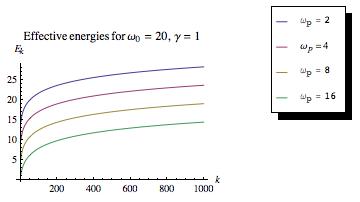
Figure 1: Effective energies for various values of the coupling $\omega_{p}$.

IV.1 High $k$ asymptotic behavior of symplectic eigenvalues

To compute the cutoff dependence of the entropy for $\chi_{b}$, we consider the large $k$ asymptotics of $g_{k},h_{k}$. Using (67) at large $k$ we rewrite $g_{k}$ as:

$$g_{k}=\int_{0}^{\infty}\frac{1}{w^{2}+k^{2}+\omega_{p}^{2}(1-B)}\,dw\,.$$ (74)

where $B=\frac{\gamma_{p}w+\omega_{0}^{2}}{w^{2}+\gamma_{p}w+\omega_{0}^{2}}$. Noting that $\omega_{p}^{2}B<\omega_{p}^{2}$, we can expand in series in $B$, obtaining, to lowest order in $B/(\omega^{2}+k^{2}+\omega_{p}^{2})$:

$$g_{k}=\int_{0}^{\infty}dw(\frac{1}{w^{2}+k^{2}+\omega_{p}^{2}}+{\omega_{p}^{2}}\frac{1}{(w^{2}+k^{2}+{\omega_{p}^{2}})^{2}}\frac{\gamma_{p}w+\omega_{0}^{2}}{w^{2}+\gamma_{p}w+\omega_{0}^{2}})+$$

$$\text{higher}\,\text{orders}\sim\frac{\pi}{2}\frac{1}{\sqrt{{\omega_{p}^{2}}+k^{2}}}+{\omega_{p}^{2}}II$$ (75)

with $II=\int_{0}^{\infty}dw{\omega_{p}^{2}}\frac{1}{(w^{2}+k^{2}+{\omega_{p}^{2}})^{2}}\frac{\gamma_{p}w+\omega_{0}^{2}}{w^{2}+\gamma_{p}w+\omega_{0}^{2}}$. let us compute II.

Writing: $\omega^{2}+\gamma_{p}\omega+\omega_{0}^{2}=\left(\omega-a_{-}\right)\left(\omega-a_{+}\right),$ where $a_{\pm}=\frac{-\gamma_{p}\pm\sqrt{\gamma_{p}^{2}-4\omega_{0}^{2}}}{2}$, there are two cases:

1) $\gamma_{p}^{2}>4\omega_{0}^{2}.$ In this case $a_{\pm}$ are real and negative and carrying the integral we get

$$\text{II}=\frac{\gamma_{p}\log k}{k^{4}}-\frac{\gamma_{p}}{2k^{4}}+$$

$$\frac{-\log\left[-a_{-}\right]a_{-}^{2}+\log\left[-a_{+}\right]a_{+}^{2}}{k^{4}\left(-a_{-}+a_{+}\right)}$$ (76)

2) $\gamma_{p}^{2}<4\omega_{0}^{2}.$ In this case $a_{\pm}$ are complex conjugates and we find

$$\text{II}=\frac{\gamma_{p}\log k}{k^{4}}-{\gamma_{p}+\gamma_{p}\log\omega_{0}^{2}\over 2k^{4}}+$$

$$\frac{1}{k^{4}\sqrt{4\omega_{0}^{2}-\gamma_{p}^{2}}}(\gamma_{p}^{2}-2\omega_{0}^{2}){arg}[\frac{\gamma_{p}}{2}-\frac{i}{2}\sqrt{4\omega_{0}^{2}-\gamma_{p}^{2}}]$$ (77)

In particular, if $\gamma_{p}=0$ we have: $II=\frac{\pi\omega_{0}}{2k^{4}}$. Similarly, we write:

$$h_{k}=\left(k^{2}+{\omega_{p}^{2}}\right)g_{k}-{\omega_{p}^{2}}\text{III}$$ (78)

where to lowest order:

$$\text{III}=\int_{0}^{\infty}\frac{\gamma_{p}w+\omega_{0}^{2}}{w^{2}+\gamma_{p}w+\omega_{0}^{2}}\frac{1}{w^{2}+k^{2}+{\omega_{p}^{2}}}dw$$

Carrying through the integrals we find again two cases: 1) $\gamma_{p}{}^{2}>4\omega_{0}{}^{2}.$ Then $a_{\pm}$ are real and negative and

$$\text{III}=\frac{\log[k]\gamma_{p}}{k^{2}}-\frac{\log\left[-a_{-}\right]a_{-}^{2}}{k^{2}\sqrt{\gamma_{p}{}^{2}-4\omega_{0}{}^{2}}}+\frac{\log\left[-a_{+}\right]a_{+}^{2}}{k^{2}\sqrt{\gamma_{p}{}^{2}-4\omega_{0}{}^{2}}}$$ (79)

2) $\gamma_{p}{}^{2}<4\omega_{0}{}^{2}.$ $a_{\pm}$ are complex conjugates. we find:

$$\text{III}=\frac{\gamma_{p}\log[k]}{k^{2}}-\frac{2\gamma_{p}\log\left[\omega_{0}\right]}{2k^{2}}+$$

$$\frac{\left(\gamma_{p}^{2}-2\omega_{0}{}^{2}\right)\text{arg}\left[\gamma_{p}-i\sqrt{4\omega_{0}{}^{2}-\gamma_{p}{}^{2}}\right]}{k^{2}\sqrt{4\omega_{0}{}^{2}-\gamma_{p}{}^{2}}}$$ (80)

3) $g=0$. In this case:

$$\text{III}=\frac{\pi\omega_{0}}{2k^{2}}$$ (81)

Computing to lowest order in $\omega_{p}$ the corrections $II,III$, we find for large $k$, small $\omega_{p}$ and $\gamma_{p}\neq 0$

$$g_{k}h_{k}=\frac{\pi^{2}}{4}+\frac{\omega_{p}^{2}\gamma_{p}\pi\log k}{2k^{3}}.$$ (82)

We remark that if $\gamma_{p}=0$ we get a slightly modified result: $g_{k}h_{k}=\frac{\pi^{2}}{4}+\frac{4\pi\omega_{0}\pi^{2}}{4k^{3}}.$

We conclude that the symplectic eigenvalues $\mu_{\bf k}$, to lowest order in $\omega_{p}$, behave as:

$$\mu_{\bf k}\sim 1+{\omega_{p}^{2}\gamma_{p}\log k\over\pi}+..$$ (83)

for $k\gg 1$.

IV.2 Low $k$ behavior of symplectic eigenvalues

Studying the low $k$ behavior requires slightly more care in the expansion. Here we find that the leading behavior for the field correlators at low $k$ is given by

$$g_{k}\sim\frac{\pi}{2k\sqrt{1+\frac{\omega_{p}^{2}}{\omega_{0}^{2}}}}.$$ (84)

To do so, we start by rescaling $w$ in the integral (67):

$$g_{k}=\int_{0}^{\infty}\frac{1}{w^{2}+k^{2}+\frac{w^{2}{\omega_{p}^{2}}}{w^{2}+\gamma_{p}w+\omega_{0}^{2}}}dw=$$

$$\frac{1}{k}\int_{0}^{\infty}\frac{1}{1+x^{2}+x^{2}\frac{{\omega_{p}^{2}}}{\omega_{0}^{2}}\left(1-\frac{kx(kx+\gamma_{p})}{k^{2}x^{2}+\gamma_{p}kx+\omega_{0}^{2}}\right)}dx.$$ (85)

We continue to split the integral into two intervals $(0,k^{-1})$ and $(k^{-1},\infty)$, and separately approximating each term:

$$\frac{1}{k}\int_{0}^{1/k}\frac{1}{1+x^{2}+x^{2}\frac{{\omega_{p}^{2}}}{\omega_{0}^{2}}(1-\frac{kx(kx+g)}{k^{2}x^{2}+\gamma_{p}kx+\omega_{0}^{2}})}dx+$$

$$\frac{1}{k}\int_{1/k}^{\infty}\frac{1}{1+x^{2}+x^{2}\frac{{\omega_{p}^{2}}}{\omega_{0}^{2}}(1-\frac{kx(kx+\gamma_{p})}{k^{2}x^{2}+\gamma_{p}kx+\omega_{0}^{2}})}dx$$

$$\sim\frac{1}{k}\int_{0}^{1/k}\frac{1}{1+x^{2}+x^{2}\frac{{\omega_{p}^{2}}}{\omega_{0}^{2}}}dx+\frac{1}{k}\int_{1/k}^{\infty}\frac{1}{1+x^{2}}dx$$ (86)

for small k we get:

$$\frac{1}{k}\int_{1/k}^{\infty}\frac{1}{1+x^{2}}dx\to 1$$ (87)

and:

$$\frac{1}{k}\int_{0}^{1/k}\frac{1}{1+x^{2}+x^{2}\frac{{\omega_{p}^{2}}}{\omega_{0}^{2}}}dx=\frac{\text{arctan}\left[\frac{1}{k}\sqrt{1+\frac{\omega_{p}^{2}}{\omega_{0}^{2}}}\right]}{k\sqrt{1+\frac{{\omega_{p}^{2}}}{\omega_{0}^{2}}}}\to$$

$$\frac{\pi}{2k\sqrt{1+\frac{\omega_{p}^{2}}{\omega_{0}^{2}}}}$$ (88)

a similar treatment shows that:

$$h_{k}\sim\frac{\pi\omega_{p}^{2}}{\sqrt{4\omega_{p}^{2}-\gamma_{p}^{2}+4\omega_{0}^{2}}}+o(k).$$ (89)

Finally, we find that the symplectic eigenvalues diverge at $k\rightarrow 0$ since

$$\sqrt{g_{k}h_{k}}\sim\frac{\pi}{\sqrt{2k}}\left(\frac{\omega_{0}^{2}({\omega_{p}^{2}})^{2}}{(\omega_{0}^{2}+{\omega_{p}^{2}})\left(4\omega_{p}^{2}-\gamma_{p}^{2}+4\omega_{0}^{2}\right)}\right)^{1/4}$$ (90)

diverges as $\frac{1}{\sqrt{2k}}$ for small $k$. The entropy function $h(k)$ for small $k$s diverges as $h(k)\sim-log(k)$. However, integration $d^{D}k$ is finite for any dimension and so there are no infra-red divergences in the total entropy per unit volume.

IV.3 Interpretation of the field reduced density matrix

Having evaluated the symplectic eigenvalues of the field covariance matrix we can write the density matrix of the field as (48)

$$\rho=Z^{-1}e^{-\sum_{k}2\Lambda_{k}{a^{+}}_{k}a_{k}}~{};~{}2\Lambda_{k}=\log{\sqrt{\frac{4}{\pi^{2}}g_{k}h_{k}}+1\over\sqrt{\frac{4}{\pi^{2}}g_{k}h_{k}}-1}$$ (91)

As mentioned in the introduction, the first natural question to ask is: is the state of the field $\rho$ thermal? This is certainly a natural possibility suggested by considering the bulk material as a thermal bath for the field. In fact, one may always write the state $\rho$, formally, as thermal, i.e.:

$$\rho=Z^{-1}exp(-\beta H_{eff}),$$ (92)

for some suitable operator $H_{eff}$. However, to actually interpret the state as thermal, we would like $H_{eff}$ to represent a reasonable, local, physical Hamiltonian. For the Gaussian states we can write $H_{eff}$ explicitly as:

$$H_{eff}=\int{\rm d}{\bf x}{\rm d}{\bf x}^{\prime}\hat{u}({\bf x}-{\bf x}^{\prime})a^{+}_{{\bf x}}a_{{\bf x}^{\prime}}$$ (93)

where

$$\hat{u}=2\beta^{-1}\int{\rm d}{\bf k}\Lambda_{\bf k}e^{i{\bf k}\cdot({\bf x}-{\bf x}^{\prime})}.$$ (94)

The locality properties of this Hamiltonian thus depend on the locality of the Fourier transform. We find that generically the Fourier transformed $\hat{u}$ gives us a non-local $H_{eff}$.

Alternatively, we may interpret $2\Lambda_{\bf k}$ as $2\Lambda_{\bf k}=\beta_{k}\omega_{k}$ where $\omega_{k}$ are the photon energies in a free homogenous space, without the interaction with the material, i.e.

$$\beta_{k}\omega_{k}=2\Lambda_{k}\sim\log\left(\frac{\sqrt{\frac{4}{\pi^{2}}g_{k}h_{k}}+1}{\sqrt{\frac{4}{\pi^{2}}g_{k}h_{k}}-1}\right)$$ (95)

As is clearly shown in fig.1, if we take $\omega_{k}\propto|k|$ we find that different momenta ${\bf k}$ feel different effective temperatures.

In the infra-red limit expanding this expression for small $k$ using we find the leading, small $k$ behavior:

$$\beta_{k}\omega_{k}\sim\nu\sqrt{k}~{}~{};$$

$$\nu\equiv\sqrt{2}\left(\frac{\omega_{0}^{2}(\omega_{p}^{2})^{2}}{(\omega_{0}^{2}+\omega_{p}^{2})\left(4\omega_{p}^{2}-\gamma_{p}^{2}+4\omega_{0}^{2}\right)}\right)^{-1/4}$$ (96)

If we assume $\omega_{k}\propto|k|$ we conclude that the effective temperature of this $k$ mode is:

$$T_{k}\equiv{k\over\beta_{k}}\propto{\sqrt{k}}~{}~{}~{}as~{}~{}~{}~{}k\rightarrow 0.$$ (97)

What is the energy and number of occupied soft modes per unit volume up to a given $k_{m}$? We show that these are proportional to $k_{m}^{d+1/2}$ and $k_{m}^{d-1/2}$, respectively, are finite and small. Indeed, since the occupation of a mode k is given by:

$$n_{k}=\frac{1}{e^{\beta_{k}\omega_{k}}-1}\sim\frac{1}{\nu\sqrt{k}}$$ (98)

The expected occupation number for modes with $k<k_{\min}$ is thus given by:

$$\text{ }N_{\text{kmin}}=\int_{k<k_{\min}}d^{d}kn_{k}\propto\int_{0}^{k_{\min}}\text{dk}\frac{k^{d-1}}{\nu\sqrt{k}}=\frac{k^{d-1/2}}{\nu\left(d-\frac{1}{2}\right)}$$ (99)

The energy, assuming $\omega_{k}\propto k$, is:

$$E\left(k<k_{\min}\right)\sim\int_{k<k_{\min}}d^{d}kn_{k}k\propto$$

$$\int_{0}^{k_{\min}}\text{dk}\frac{k^{d}}{\nu\sqrt{k}}=\frac{k^{d+1/2}}{\nu\left(d+\frac{1}{2}\right)}$$ (100)

Finally, the number variance of modes up to $k_{m}$ is computed as:

$$\delta N^{2}\left(k<k_{\min}\right)=\int_{k<k_{\min}}d^{d}kn_{k}\left(1+n_{k}\right)\propto$$

$$\int_{0}{}^{k_{\min}}\text{dk}k^{d-1}\frac{1}{\mu^{2}k}=$$

$$\int_{0}{}^{k_{\min}}\text{dk}k^{d-2}\frac{1}{\mu^{2}}=\begin{cases}\frac{1}{\mu^{2}}\log\frac{k_{\min}}{\varepsilon_{IR}}&d=1\\ \frac{1}{\mu^{2}}\frac{\left(k_{\min}\right){}^{d-1}}{d-1}&d>1\end{cases}.$$ (101)

Note that for $d=1$ we find an infra-red divergence: $\langle\delta N^{2}\rangle=-\log\varepsilon_{IR}$, where $\varepsilon_{IR}$ is an infra-red cutoff, inversely proportional to the system size.

IV.4 Cutoff dependence of the entropy

In this section, we compute the total field entropy, and show that it suffers from a UV divergence. This result is not surprising, since, in principle, entanglement can get contributions from all momentum scales.

Using (70), the full quantum von-Neumann entropy of the field per unit volume is given by the momentum integrals of $h(\sqrt{\frac{4}{\pi^{2}}g_{k}h_{k}})$. The large momentum behavior of the integrand is obtained from (82) to be:

$$h(\sqrt{\frac{4}{\pi^{2}}g_{k}h_{k}})\sim\frac{\omega_{p}^{2}\gamma_{p}\log k(1+3\log k-\log\frac{\omega_{p}^{2}\gamma_{p}\log k}{2\pi})}{2\pi k^{3}}$$ (102)

for a transparent medium ($\gamma_{p}<<1$) we consider additional terms and find:

$$h(\sqrt{\frac{4}{\pi^{2}}g_{k}h_{k}})\sim\frac{{\omega_{p}^{2}}{\omega_{0}}(1+3\log k-\log\frac{\omega_{p}^{2}{\omega_{0}}}{4})}{4k^{3}}$$ (103)

using the integrals $\int\frac{\log[k]}{k}=\frac{\log[k]^{2}}{2}$ and $\int\frac{\log^{2}[k]}{k}=\frac{\log[k]^{3}}{3}$, we can estimate the integration of the expressions (102), (103) over $k$ in 3d, to find the entropy per unit volume

$${\cal S}_{field}\propto\Big{\{}\begin{array}[]{cc}\omega_{p}^{2}\gamma_{p}\log(\Lambda)^{3}&\\ \omega_{p}^{2}\omega_{0}\log(\Lambda)^{2}&\gamma_{p}=0\\ 0&plasma\,\,model\end{array},$$ (107)

where $\Lambda$ is a high momentum (UV) cutoff.

Note that in obtaining (107) is obtained to lowest order in $\omega_{p}$. However, this approximation is justified for our purposes since it becomes exact at the large $k$ limit which we are studying. Indeed, numerically, the approximations used in (107) actually recover the correct cutoff dependence even for large values of $\omega_{p}$, since the dielectric response decays at large $k$ values.

It is interesting to observe the special place of the ”pure plasma” limit response function. We can easily understand the result (107) as follows: Substituting the plasma permittivity limit form $\chi=-{\omega_{c}^{2}\over\omega^{2}}$ in the action (2), in a homogenous space, we see that the role of $\chi$ is similar to producing a mass term for $\phi$. Thus, the resulting action is consistent with a Hermitian field Hamiltonian, and as such, at zero temperature, to a pure state. One can also understand the vanishing of entropy for pure plasma as follows: Consider a slab of material, with a pure plasma form for the dielectric response. Such a material will have no losses: A pure plasma system will be completely transparent to radiation above the plasma frequency, and completely reflecting at lower frequencies. The field will have a finite mass inside the region occupied by the plasma and will not generate entropy. It is interesting that the use of a pure plasma in the computations of Casimir energy and Entropy has been at the heart of a recent debate Bezerra et al. (2004); Decca et al. (2005); Brevik et al. (2005); Sushkov et al. (2011). We do not make any claims regarding the debate, but note that the distinction between the Casimir entropy in the two models is manifested in the full quantum entropy computed herein.

We remark that it is possible to incorporate the high momentum cutoff more naturally by taking into account the spatial dispersion in $\varepsilon$. While different functions may have different asymptotic properties, we expect to get similar behavior. Indeed, if we take, for concreteness sake, the simplest extension of the previous treatment, we can use (see e.g. Klingshirn (2005)).

$$\varepsilon(i\omega,k)=\varepsilon_{0}\left(1+\frac{f}{\text{A k}^{2}+\gamma\omega+\omega^{2}+\omega_{0}^{2}}\right)$$ (108)

where the expression is valid for small $k\ll\pi/a$ where $a$ is the interatomic distance. One can easily check that this form doesn’t change much the cutoff dependence.

V Distance dependent entropies

Since the entropy ${{\cal S}_{field}}$ is UV divergent, it is natural to ask, in analogy with the Casimir effect, what is the distance dependence of the entropy of interaction with two distinct bodies $A$ and $B$, and is the distance dependent part of it is UV finite. To answer such questions, the “Casimir EE” was defined in Klich (2012) as

$${\cal S}_{{R,\alpha}}(A,B)={\cal S}_{\alpha}(A\cup B)-{\cal S}_{\alpha}(A)-{\cal S}_{\alpha}(B),$$ (109)

where ${\cal S}_{{\alpha}}(M)$ is the $\alpha-$Renyi entropy of a field interacting with a body $M$ described by $\varepsilon=\varepsilon_{0}+\chi_{M}$, where the susceptibility $\chi_{M}=0$ everywhere outside $M$. The situation is illustrated in Fig.2

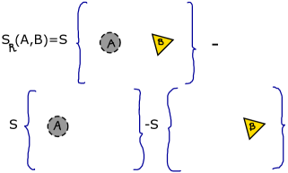
Figure 2: A Casimir entanglement entropy.

The following few remarks regarding ${\cal S}_{{R}}$ are important to note:

1. ${\cal S}_{{R}}$ is distinct from the more familiar Casimir entropy. Casimir entropy is defined as ${\cal S}_{C}(A,B)=-\lim_{T\rightarrow 0}\partial_{T}F_{C}$, where $F_{C}$ is the Casimir free energy, obtained by subtracting all distance independent terms from the free energy of the EM field in the presence of bodies $A,B$ or boundary conditions.

2. ${\cal S}_{{R}}$ is different from the ”relative entropy” of probability theory, as we are comparing different systems, and not merely different statistical information about the same system.

3. It is important to note that, while the sub-additivity of von-Neumann entropy Araki and Lieb (1970) shows that the entropy ${\cal S}$ of a field is always larger than the total entropy of the combined system of field matter, this is no longer evident once subtractions are taking place in order to define ${\cal S}_{R}$.

The relevance of Casimir entropy ${\cal S}_{C}$ to understanding thermal corrections of the Lifshitz formula has been pointed out in many papers (see e.g. Bezerra et al. (2004); Geyer et al. (2005); Bordag and Pirozhenko (2010)), where it was noticed that as $T\rightarrow 0$, ${\cal S}_{C}$ may not go to zero when using the Drude model, as would be expected by the Nernts theorem. It is quite interesting to note that while the Casimir entanglement entropy ${\cal S}_{{R}}$ is distinct from ${\cal S}_{C}$, a similar behavior is observed in (107). ${\cal S}_{C}$ has a clear thermodynamic meaning, especially at high temperatures, where the Casimir force is entirely entropic Feinberg et al. (2001). Indeed, at high temperatures we expect ${\cal S}_{R}={\cal S}_{C}$, as most of the field entropy will be thermal (Technically, the relevant Green’s function gets its major contribution from the $\omega=0$ Matsubara pole).

VI Formulas for the distance dependent Von Neumann and Renyi entropies

In this section we describe the derivation of an abstract formula presented in Klich (2012) for the Casimir entanglement entropy. In addition, we generalize the formula to also describe arbitrary Renyi entropies. It was shown in that Klich (2012) :

$${\cal S}_{R}(A,B)=-\frac{1}{\pi}\int_{1/2-\text{i$\infty$}}^{1/2+\text{i$\infty$}}dx\frac{\log\left[\frac{\sqrt{x}+\frac{1}{2}}{\sqrt{x}-\frac{1}{2}}\right]}{2\sqrt{x}}{\rm Tr}\log$$

$$\left(1-\frac{1}{1-K_{A}}\left(K_{A}K_{B}+K_{\text{AUB}}-K_{A}-K_{B}\right)\frac{1}{1-K_{B}}\right)$$ (110)

where $K_{A}=\frac{1}{x-1/4+is}\left(\Gamma_{A}-1/4\right)$, and similar expressions hold for $K_{B},K_{AUB}$. Here $\Gamma={\cal G}_{A}{\cal H}_{A}$, where ${\cal G}_{A}$ and ${\cal H}_{A}$ are field and field momentum two point functions, respectively, in the presence of body $A$.

In this section we repeat the derivation of (VI) and generalize the expression to general Renyi entropies:

$$S_{R,\alpha}=-\frac{1}{\pi}\int_{1/2-\text{i$\infty$}}^{1/2+\text{i$\infty$}}{\rm d}x\frac{\left(\left(2\sqrt{x}+1\right)^{\alpha-1}-\left(2\sqrt{x}-1\right)^{\alpha-1}\right)\alpha}{\left(\left(2\sqrt{x}+1\right)^{\alpha}-\left(2\sqrt{x}-1\right)^{\alpha}\right)\sqrt{x}(\alpha-1)}{\rm Tr}\log$$

$$\left(1-\frac{1}{1-K_{A}}\left(K_{A}K_{B}+K_{\text{AUB}}-K_{A}-K_{B}\right)\frac{1}{1-K_{B}}\right)$$ (111)

The expression (VI), is similar to the TGTG formulas in it’s form: an integral over the TrLog of a combination of Green’s functions. However, it differs from such formulas in three major aspects:

1) The integration variable $x$ is not a frequency variable, but rather an auxiliary spectral variable,

2) The presence of the term $K_{AUB}$ does not allow for full separation into local object properties and free propagators.

3) The non-analyticity of the integrand at $x=1/4$. All of these make the formula harder to use than the TGTG formulas. Nevertheless, it can be used as a starting point for various expansions when the bodies are weakly entangled with the field, so that $||\Gamma_{A}-1/4||\ll 1$.

The derivation bellow of eq. (VI) follows and adapts the approach of Kenneth and Klich (2008) to the scattering formalism for Casimir energies.

To compute the entropy, we first need to find an expression for the density of symplectic eigenvalues of the covariance matrix $\gamma$. In the absence of $\langle\phi\pi\rangle$ correlations, these symplectic eigenvalues (up to a factor 2 in the definition of the covariance matrix eq. (11)) are related to the square roots of eigenvalues of $\Gamma$.

Thus, we first find a convenient representation to the density of density of states of $\Gamma={\cal G}{\cal H}$. Note that $\Gamma$ is not Hermitian, however, since ${\cal G}$ and ${\cal H}$ are positive Hermitian matrices, it has the same spectrum as ${\cal G}^{1/2}{\cal H}{\cal G}^{1/2}$, and one may safely use the formulas below. Consider the representation:

$$\delta(E-x)=\frac{1}{\pi}\text{Im}\frac{1}{E-x+i0}=$$

$$\frac{1}{\pi}\text{Im}\partial_{E}\text{Log}(E-x+i0)$$ (112)

Then we have: relative density of states of a Hermitian operator X as:

$$\delta\rho_{\Gamma}(E)\equiv\rho_{\Gamma}(E)-\rho_{\Gamma_{0}}(E)=$$

$$\frac{1}{\pi}\text{Im}\partial_{E}\left[\text{TrLog}(E-\Gamma+i0)-\text{TrLog}\left(E-\Gamma_{0}+i0\right)\right]=$$

$$\frac{1}{\pi}\text{Im}\partial_{E}\text{TrLog}\left(({E-\Gamma+i0})({E-\Gamma_{0}+i0})^{-1}\right)$$

$$=\frac{1}{\pi}\text{Im}\partial_{E}\text{TrLog}\left(1+\left(\Gamma_{0}-\Gamma\right)\frac{1}{E-\Gamma_{0}+i0}\right)$$ (113)

Denoting: $G_{0}=\frac{1}{E-\Gamma_{0}+is}$ and $D=\left(\Gamma-\Gamma_{0}\right)$, we can write (VI) as

$$\delta\rho_{\Gamma}(E)=\frac{1}{\pi}\text{Im}\partial_{E}\text{TrLog}\left(1-G_{0}D\right)$$

To compute

$${\cal S}_{{R}}(A,B)={\cal S}(A\cup B)-{\cal S}(A)-{\cal S}(B),$$ (114)

we need the relative densities:

$$\delta\rho_{R}\equiv\delta\rho_{\Gamma_{AUB}}-\delta\rho_{\Gamma_{A}}-\delta\rho_{\Gamma_{B}}=$$

$$\frac{1}{\pi}\text{Im}\partial_{E}[\text{Tr log}\left(1-G_{0}D_{AUB}\right)-\text{Tr log}\left(1-G_{0}D_{A}\right)$$

$$-\text{Tr log}\left(1-G_{0}D_{B}\right)].$$ (115)

Here $D_{A}$ is computed using $\Gamma_{A}={\cal G}_{A}{\cal H}_{A}$, where the correlations ${\cal G}_{A},{\cal H}_{A}$ are computed for the field in the presence of body $A$, and similarly for $D_{AUB},D_{B}$. We combine the terms using the following identity:

$$\frac{1}{1-G_{0}D_{A}}\left(1-G_{0}D_{\text{AUB}}\right)\frac{1}{1-G_{0}D_{B}}=$$

$$\frac{1}{1-G_{0}D_{A}}((1-G_{0}D_{A})\left(1-G_{0}D_{B}\right)-$$

$$G_{0}D_{A}G_{0}D_{B}-G_{0}(D_{\text{AUB}}-D_{A}-D_{B}))\frac{1}{1-G_{0}D_{B}}=$$

$$1-\frac{1}{1-G_{0}D_{A}}\left(G_{0}D_{A}G_{0}D_{B}+D_{\text{AUB}}-D_{A}-D_{B}\right)\frac{1}{1-G_{0}D_{B}}$$

Defining:

$$K_{A}=G_{0}D_{A}=\frac{1}{E-\Gamma_{0}+is}\left(\Gamma_{A}-\Gamma_{0}\right)$$

we obtain

$$\delta\rho(E)_{R}=\frac{1}{\pi}\text{Im}\partial_{E}\text{TrLog}\Big{(}1-$$

$$\frac{1}{1-K_{A}}\left(K_{A}K_{B}+K_{\text{AUB}}-K_{A}-K_{B}\right)\frac{1}{1-K_{B}}\Big{)}$$

We now use this spectral density to compute the entropy using the eigenvalues of the covariance matrix, eq. (III),

$${\cal S}=\sum_{i}h(\mu_{i})~{};~{}h(\mu)={\mu+1\over 2}\log{\mu+1\over 2}-{\mu-1\over 2}\log{\mu-1\over 2}$$

The lowest eigenvalue ${\cal G}{\cal H}$ is always larger or equal to 1/2, by the uncertainty relations. Thus we may write

$$S=\int_{1/2}^{\infty}h\left(2\sqrt{x}\right)\delta\rho(x)_{R}dx$$ (116)

Integrating by parts and moving the contour integration to the imaginary axis, we write this expression as:

$$S=-\frac{1}{\pi}\int_{1/2-\text{i$\infty$}}^{1/2+\text{i$\infty$}}{\rm d}x\frac{\text{Log}\left[\frac{\sqrt{x}+\frac{1}{2}}{\sqrt{x}-\frac{1}{2}}\right]}{2\sqrt{x}}\text{TrLog}$$

$$\left(1-\frac{1}{1-K_{A}}\left(K_{A}K_{B}+K_{\text{AUB}}-K_{A}-K_{B}\right)\frac{1}{1-K_{B}}\right)$$

which is eq. (11).

We can also extend this formula to cover Renyi entropies (57). Using the formula for the density of states (VI) together with the expression for the Renyi entropy in terms of the symplectic eigenvalues (60), we find:

$$S_{R,\alpha}=$$

$$-\frac{1}{\pi}\int_{1/2-\text{i$\infty$}}^{1/2+\text{i$\infty$}}(\partial_{E}h_{\alpha}(2\sqrt{E}))\text{Tr}\text{Log}(1-$$

$${1\over 1-K_{A}}(K_{A}K_{B}+K_{\text{AUB}}-K_{A}-K_{B})\frac{1}{1-K_{B}})dE$$ (117)

yielding (VI). In particular, the second Renyi entropy is given by:

$$S_{R,2}=-\frac{1}{\pi}\int_{1/2-\text{i$\infty$}}^{1/2+\text{i$\infty$}}{\rm d}x{1\over 2x}{\rm Tr}\log(1-$$

$$\frac{1}{1-K_{A}}\left(K_{A}K_{B}+K_{\text{AUB}}-K_{A}-K_{B}\right)\frac{1}{1-K_{B}}).$$ (118)

To relate this form to TGTG formulas, we recall that in such formulas, the relative density of states of the electromagnetic field interacting with for two bodies $A,B$, through dielectric susceptibilities $\chi_{A}(\omega),\chi_{B}(\omega)$ at frequency $\omega$ is expressed (before Wick rotation) as:

$${1\over\pi}Im\partial_{\omega}\text{Tr log}(1-T_{A}G_{0}T_{B}G_{0})$$ (119)

where $T_{A}=\omega^{2}\chi_{A}{1\over 1-G_{0}\omega^{2}\chi_{A}}$ are the Lippman-Schwinger operators of the problem, and $G_{0}$ are free propagators.

Choosing $K_{A}\frac{1}{1-K_{A}}$ to play the role of $T_{A}G_{0}$ and $K_{B}\frac{1}{1-K_{B}}$ the role of $T_{B}G_{0}$, The density of states (VI) may be written as:

$$\delta\rho(E)_{R}=$$

$$\frac{1}{\pi}\text{Im}\partial_{E}\text{TrLog}(1-T_{A}G_{0}T_{B}G_{0}$$

$$-\frac{1}{1-K_{A}}\left(K_{\text{AUB}}-K_{A}-K_{B}\right)\frac{1}{1-K_{B}}).$$

We observe, however, the appearance of an additional $\left(K_{\text{AUB}}-K_{A}-K_{B}\right)$ term, which is not-separable into a product of correlators of the separate bodies.

VII Representation of the correlation functions in terms of Lippmann-Schwinger operators

In the computation of the correlation functions bellow, we will use extensively the representation of correlation functions in terms of Lippmann-Schwinger operators. For a body A, we define the Lippmann-Schwinger operator $T_{A}$ at imaginary frequency $i\omega$ by

$$T_{A}=\omega^{2}\chi_{A}{1\over 1+g_{0}\omega^{2}\chi_{A}(i\omega)}$$ (120)

where $g_{0}$ are free propagators. In particular, for a scalar field we take $g_{0}={1\over-\Delta+\omega^{2}}$.

The Lippmann-Schwinger operator $T_{A}$ is related to the green’s function $g_{A}$ ,

$$\langle x|g_{A}(\omega)|x^{\prime}\rangle=\langle x|\frac{1}{-\Delta+\omega^{2}\varepsilon_{A}(i\omega)}|x^{\prime}\rangle$$ (121)

by the operator equation:

$$g_{A}(\omega)=g_{0}(\omega)+g_{0}(\omega)T_{A}g_{0}(\omega)$$ (122)

The eq. (67) for the $\langle\phi\phi\rangle$ correlation functions written in a general basis (i.e. without assuming translational invariance) is then:

$${\cal G}_{A}=\int_{0}^{\infty}\text{d}\omega g_{A}=\int_{0}^{\infty}\text{d}\omega\left(g_{0}+g_{0}T_{A}g_{0}\right)=$$

$${\cal G}_{0}+\int_{0}^{\infty}\text{d}\omega g_{0}T_{A}g_{0}$$ (123)

Similarly, as in (IV), the field momenta correlation functions are encoded by

$${\cal H}_{A}={\cal H}_{0}-\int\text{d}\omega\omega^{2}g_{0}T_{A}g_{0}.$$ (124)

(in the expressions above, and what follows we omit the $\omega$ dependence in $g_{0}$). We note that in the continuum, ${\cal G}_{0},{\cal H}_{0}$ are diagonal in momentum, with matrix elements given by ${\pi\over 2|k|}\delta(k-k^{\prime})$ and ${\pi|k|\over 2}\delta(k-k^{\prime})$ respectively (as obtained in eq. (71),(72)).

Let us recall some general properties of $T_{A}$ on the imaginary frequency axis Kenneth and Klich (2008). Below we will repeatedly use that, as a consequence of the Kramers-Kronig relations, combined with the assumption of equilibrium we have $\chi_{A}(i\omega)>0$. In it is known that $\chi_{A}(i\omega)$ is real and decaying as $\omega^{-2}$ as $\omega\rightarrow\infty$.

We have the following properties:

1. $T_{A}\psi=0$ for any $\psi$ for which vanishes on $A$. This is established by rewriting $T_{A}$ as

$$T_{A}=\sqrt{\omega^{2}\chi_{A}}{1\over 1+\sqrt{\omega^{2}\chi_{A}}g_{0}\sqrt{\omega^{2}\chi_{A}}}\sqrt{\omega^{2}\chi_{A}}$$ (125)

2. $T_{A}$ is a positive operator, i.e. $\langle\psi|T_{A}|\psi\rangle>0$ for any $\psi$ in the Hilbert space $T_{A}$ acts on (square integrable function supported on the region A).

And,

3.

$$T_{A}<\omega^{2}\left(\varepsilon_{A}(i\omega)-1\right)$$ (126)

as operators, i.e. for any vector $\psi$, $\langle\psi|T_{A}|\psi\rangle<\langle\psi|\omega^{2}\left(\varepsilon_{A}(i\omega)-1\right)|\psi\rangle$.

In the next section we use these properties in our analysis of the distance dependence of the entropy ${\cal S}_{R}$.

VIII Large distance expansion of the Renyi entropy $S_{2,R}$

In this section, we study the behavior of the relative entanglement at large distances. Consider two bodies with a dielectric function $\varepsilon_{A}(i\omega)=1+{\omega_{pA}^{2}\over\omega^{2}+\omega_{0}^{2}}$ (and similar expression for body $B$), and volumes $V_{A},V_{B}$.

Our main result is that at large separation the Renyi entropy of the field is the sum of the separate body entropies, with the correction decaying as:

$$S_{2,R}=-\omega_{{pA}}^{2}\omega_{{pB}}^{2}V_{A}V_{B}\frac{2\pi^{4}}{\omega_{0}^{2}R^{4}}+O({1\over R^{6}})$$ (127)

Note that the power law differs from the typical power law of $R^{-7}$ appearing in the Casimir-Polder interaction.

To find this result we first write the 2-Renyi entropy (62) as:

$$S_{2}=\Sigma\log\mu=\frac{1}{2}\text{Tr}\log(1+\delta\Gamma)$$ (128)

Thus the relative $S_{2,R}$ is given by:

$$S_{2,R}=\frac{1}{2}\text{Tr}\log\left(1+\delta\Gamma_{B}\right){}^{-1}\left(1+\delta\Gamma_{\text{AUB}}\right)\left(1+\delta\Gamma_{A}\right){}^{-1}$$

$$=\frac{1}{2}\text{Tr}\log\Big{[}1+$$

$$\frac{1}{1+\delta\Gamma_{B}}\left(\delta\Gamma_{\text{AUB}}-\delta\Gamma_{A}-\delta\Gamma_{B}-\delta\Gamma_{A}\delta\Gamma_{B}\right)\frac{1}{1+\delta\Gamma_{A}}\Big{]}$$ (129)

and in particular, in the long distance expansion, we expect:

$$||\delta\Gamma_{\text{AUB}}-\delta\Gamma_{A}-\delta\Gamma_{B}-\delta\Gamma_{A}\delta\Gamma_{B}||\to 0$$ (130)

and we can approximate:

$$S_{2,R}\sim\frac{1}{2}\text{Tr}\left(\delta\Gamma_{\text{AUB}}-\delta\Gamma_{A}-\delta\Gamma_{B}-\delta\Gamma_{A}\delta\Gamma_{B}\right)$$ (131)

In calculations of (131), we have several different kinds of terms. We concentrate on the so called “dilute limit ” where it is assumed $\omega^{2}\chi(i\omega)\ll 1$. In this case we can use the approximation $T_{A}\sim\omega^{2}\chi_{A}(i\omega)$.

To lowest order in $\chi_{A},\chi_{B}$, we have the following terms:

$$S_{2,R}\sim\frac{1}{2}\text{Tr}({\cal H}_{0}(\delta{\cal G}_{\text{AUB}}-\delta{\cal G}_{A}-\delta{\cal G}_{B})+$$

$$(\delta{\cal H}_{\text{AUB}}-\delta{\cal H}_{A}-\delta{\cal H}_{B}){\cal G}_{0}-$$

$${\cal H}_{0}\delta{\cal G}_{A}{\cal H}_{0}\delta{\cal G}_{B}-\delta{\cal H}_{A}{\cal G}_{0}\delta{\cal H}_{B}{\cal G}_{0}))$$ (132)

It turns out that the leading contribution is obtained from:

$${\rm Tr}{\cal H}_{0}\delta{\cal G}_{A}{\cal H}_{0}\delta{\cal G}_{B}+\delta{\cal H}_{A}{\cal G}_{0}\delta{\cal H}_{B}{\cal G}_{0}=O\left(R^{-4}\right)$$ (133)

The calculation goes as follows. Explicitly, using (71),(72) ,(VII) and (124) :

$${\rm Tr}{\cal H}_{0}\delta{\cal G}_{A}{\cal H}_{0}\delta{\cal G}_{B}+\delta{\cal H}_{A}{\cal G}_{0}\delta{\cal H}_{B}{\cal G}_{0}=O\left(R^{-4}\right)=$$

$$\int\text{d}\omega\text{d$\omega$}^{\prime}d^{3}k\langle k|{\cal H}_{0}g_{0}T_{A}g_{0}{\cal H}_{0}g_{0}T_{B}g_{0}+$$

$$\omega^{2}\omega^{\prime 2}{\cal G}_{0}g_{0}T_{A}g_{0}{\cal G}_{0}g_{0}T_{B}g_{0}|k\rangle=$$

$$\int\text{d}\omega\text{d$\omega$}^{\prime}\text{ }d^{3}kd^{3}q\text{ }\frac{1}{k^{2}+\omega^{2}}T_{A}(k,q,\omega)\frac{1}{q^{2}+\omega^{2}}\times$$

$$\frac{1}{q^{2}+\omega^{\prime 2}}T_{B}(q,k,\omega^{\prime})\frac{1}{k^{2}+\omega^{\prime 2}}\left(\frac{\omega^{2}\omega^{\prime 2}}{|k||q|}+|k||q|\right)$$ (134)

Now consider the effect of shifting the object $B$ by a vector ${R}\hat{n}$ to $B_{R}=\{x:x-{R}\hat{n}\in B\}$ . The Lippmann-Schwinger operator $T_{B_{R}}$ associated with the shifted body, written in momentum representation, is

$$T_{B_{R}}(q,k,\omega^{\prime})=\int\text{dxdy}e^{i(k\cdot x-q\cdot y)}T_{B}(x+{R}\hat{n},y+{R}\hat{n},\omega^{\prime})=$$

$$\int\text{dxdy}e^{i(k\cdot x-q\cdot y)-i(k-q)\cdot{R}\hat{n}}T_{B}(x,y,\omega^{\prime})=$$

$$e^{-i(k-q)\cdot{R}\hat{n}}T_{B}(q,k,\omega^{\prime})$$

We therefore write for the shifted position:

$$K(R)=$$

$$\int\text{d}\omega\text{d$\omega$}^{\prime}\text{ }d^{3}kd^{3}q\text{ }\frac{1}{k^{2}+\omega^{2}}T_{A}(k,q,\omega)\frac{1}{q^{2}+\omega^{2}}\times$$

$$\frac{e^{-i(k-q)\cdot R\hat{n}}}{q^{2}+\omega^{\prime 2}}T_{B}(q,k,\omega^{\prime})\frac{1}{k^{2}+\omega^{\prime 2}}\left(\frac{\omega^{2}\omega^{\prime 2}}{|k||q|}+|k||q|\right)$$ (135)

We now rescale all momenta and frequencies appearing in the integral by: $\tilde{k}=Rk.$

$$K=\int d\tilde{\omega}d\tilde{\omega}^{\prime}\text{ }d^{3}\tilde{k}d^{3}\tilde{q}\text{ }\frac{1}{R^{2}}\frac{1}{\tilde{k}^{2}+\omega^{2}}T_{A}\left(\frac{\tilde{k}}{R},\frac{\tilde{q}}{R},\frac{\tilde{\omega}}{R}\right)\times$$

$$\frac{1}{\tilde{q}^{2}+\tilde{\omega}^{2}}\frac{e^{-i\left(\tilde{k}-\tilde{q}\right)\cdot\hat{n}}}{\tilde{q}^{2}+\tilde{\omega}^{\prime 2}}T_{B}\left(\frac{\tilde{q}}{R},\frac{\tilde{k}}{R},\frac{\tilde{\omega}^{\prime}}{R}\right)\frac{1}{\tilde{k}^{2}+\tilde{\omega}^{\prime 2}}\left(\frac{\tilde{\omega}^{2}\tilde{\omega}^{\prime 2}}{\left|\tilde{k}\right|\left|\tilde{q}\right|}+\left|\tilde{k}\right|\left|\tilde{q}\right|\right)$$

Note that for $R\to\infty$ we have $T_{B}\left(\frac{\tilde{q}}{R},\frac{\tilde{k}}{R},\frac{\tilde{\omega}^{\prime}}{R}\right)\longrightarrow\left(\frac{\tilde{\omega}^{\prime}}{R}\right)^{2}\chi_{B}\left(\frac{\tilde{q}}{R},\frac{\tilde{k}}{R};\frac{\tilde{\omega}^{\prime}}{R}\right)$ since in this limit $\chi\to 0$ and $T_{B}$ can be approximated as in the dilute limit. For concreteness, let us take

$$\chi_{A}(x,\omega)=\theta_{A}(x)\frac{\omega_{pA}^{2}}{\omega^{2}+\omega_{0}^{2}}$$

$$\theta_{A}(x)=\left\{\begin{array}[]{c}1~{}~{}~{}~{}~{}~{}~{}x\in A\\ 0~{}~{}~{}\text{otherwise}\end{array}\right.$$ (138)

We can now carry out the frequency integrals yielding:

$$K=\frac{\omega_{\text{pA}}{}^{2}\omega_{pB}^{2}}{R^{2}}\int d^{3}\tilde{k}d^{3}\tilde{q}\theta_{A}\left(\frac{\tilde{k}}{R},\frac{\tilde{q}}{R}\right)\theta_{B}\left(\frac{\tilde{q}}{R},\frac{\tilde{k}}{R}\right)e^{-i\left(\tilde{k}-\tilde{q}\right)\cdot\hat{n}}\times$$

$$\frac{\pi^{2}\left(2k^{2}q^{2}+2kq(k+q)R\omega_{0}+(k+q)^{2}R^{2}\omega_{0}{}^{2}\right)}{4kq(k+q)^{2}\left(k+R\omega_{0}\right){}^{2}\left(q+R\omega_{0}\right){}^{2}}$$ (139)

For $R\rightarrow\infty$ we can use the approximation

$$\theta_{A}\left(\frac{\tilde{k}}{R},\frac{\tilde{q}}{R}\right)=\int_{A}\text{dx}e^{i\frac{x}{R}\cdot\left(\tilde{k}-\tilde{q}\right)}\sim V_{A}$$ (140)

where $V_{A}$ is the volume of body $A$. We therefore have:

$$K\sim V_{A}V_{B}\frac{\pi^{2}\omega_{{pA}}^{2}\omega_{{pB}}^{2}}{R^{2}}\int d^{3}kd^{3}q\times$$

$$\frac{\left(2k^{2}q^{2}+2kq(k+q)R\omega_{0}+(k+q)^{2}R^{2}\omega_{0}^{2}\right)}{4kq(k+q)^{2}(k+R\omega_{0})^{2}(q+R\omega_{0})^{2}}e^{-i(k-q)\cdot\hat{n}}$$ (141)

We can now carry out the 3d angular integrals in the standard way, writing: $q\cdot\hat{n}=\cos\theta|q|$, we get:

$$K=\omega_{{pA}}^{2}\omega_{{pB}}^{2}V_{A}V_{B}\frac{4\pi^{4}}{R^{2}}\int_{0}^{\infty}\text{dk}\text{dq}\times$$

$$\frac{(2k^{2}q^{2}+2kq(k+q)R\omega_{0}+(k+q)^{2}R^{2}\omega_{0}^{2})}{(k+q)^{2}(k+R\omega_{0})^{2}(q+R\omega_{0})^{2}}\sin(k)\sin(q)$$ (142)

At this point, it is convenient to rescale back the momenta, writing:

$$K=\omega_{{pA}}^{2}\omega_{{pB}}^{2}V_{A}V_{B}\frac{4\pi^{4}}{R^{2}}\int_{0}^{\infty}\text{dk}\text{dq}\times$$

$$\frac{\left(2k^{2}q^{2}+2kq(k+q)+(k+q)^{2}\right)}{(k+q)^{2}(k+1)^{2}(q+1)^{2}}\sin(k{}R\omega_{0})\sin(qR\omega_{0})$$ (143)

To analyze this integral we do a couple of integrations by parts according to:

$$\iint_{0}^{L}\text{dxdy}F(x,y)\partial_{x}\partial_{y}G(x,y)=\left(F(x,y)G(x,y)|_{x=0}^{L}\right)|_{y=0}^{L}-$$

$$\int_{0}^{L}\text{dy}\left(\partial_{y}F(x,y)\right)G(x,y)|_{x=0}^{L}-$$

$$\int_{0}^{L}\text{dx}\left(\left(\partial_{x}F(x,y)\right)G(x,y)|_{y=0}^{L}\right)+$$

$$\int_{0}^{L}\text{dx}\int_{0}^{L}\text{dy}\left(\partial_{x}\partial_{y}F(x,y)\right)G(x,y)$$ (144)

In our case we take:

$$F=\frac{\left(2k^{2}q^{2}+2kq(k\text{ }+q)+(k+q)^{2}\right)}{\text{ }(k+q)^{2}(k+1)^{2}(q+1)^{2}}$$ (145)

and

$$G=\frac{1}{(R\omega_{0})^{2}}\cos(k\text{ }R\omega_{0})\cos(qR\omega_{0}).$$ (146)

Note that $F=0$ at $k\to\infty$ at $q\to\infty$ as well as $F(0,0)=1$ and $G(0,0)=\frac{1}{(R\omega_{0})^{2}}$ Thus we have:

$$K=V_{A}V_{B}\frac{4\pi^{4}\omega_{pA}^{2}\omega_{pB}^{2}}{\omega_{0}^{2}R^{4}}+$$

$$V_{A}V_{B}\frac{4\pi^{4}\omega_{pA}^{2}\omega_{pB}^{2}}{\omega_{0}^{2}R^{4}}\Big{(}\int_{0}^{\infty}\text{dk}\text{dq}(\partial_{k}\partial_{q}F)\cos(kR\omega_{0})\cos(qR\omega_{0})$$

$$+2\int_{0}^{\infty}\text{dk}(\partial_{k}F(k,0))\cos(kR\omega_{0})\Big{)}$$ (147)

The remaining integrals in (VIII) can straightforwardly be shown to decay as $R^{-2}$ (using more integrations by parts), showing that:

$$K=V_{A}V_{B}\frac{4\pi^{4}\omega_{pA}^{2}\omega_{pB}^{2}}{\omega_{0}^{2}R^{4}}+O({1\over R^{6}}),$$ (148)

establishing the asymptotics (127).

The complete analysis we check that the additional terms in (VIII) give a sub-leading correction to (127). Indeed, the term

$$\text{Tr}{\cal H}_{0}(\delta{\cal G}_{\text{AUB}}-\delta{\cal G}_{A}-\delta{\cal G}_{B})$$

$$=\text{Tr}{\cal H}_{0}\int\text{d}\omega g_{0}\left(T_{\text{AUB}}-T_{A}-T_{B}\right)g_{0}$$ (149)

gives us a $R^{-6}$ decay. The analysis goes as follows. Using cyclicity of the trace this expression is the same as:

$$\int_{0}^{\infty}\text{d}\omega\text{Tr}\left(T_{\text{AUB}}-T_{A}-T_{B}\right)g_{0}{\cal H}_{0}g_{0}$$ (150)

where we also used that $[g_{0},{\cal H}_{0}]=0$. Using (72) for ${\cal H}_{0}$, we have

$$\langle x|g_{0}(\omega){\cal H}_{0}g_{0}(\omega)|y\rangle=$$

$$\int\frac{d^{3}k}{(2\pi)^{3}}\text{ }|k|\frac{1}{\left(k^{2}+\omega^{2}\right)^{2}}e^{i(x-y)\cdot k}=$$

$$\frac{1}{4\pi^{2}}\int_{0}^{\infty}\text{dk}\int_{-1}^{1}dX\frac{k^{3}}{\left(k^{2}+\omega^{2}\right)^{2}}e^{i|x-y|Xk}=$$

$$\frac{1}{2\pi^{2}|x-y|}\int_{0}^{\infty}\text{dk}\text{ }\frac{k^{2}}{\left(k^{2}+\omega^{2}\right)^{2}}\sin(|x-y|k)=$$

$$\frac{1}{2\pi^{2}\omega|x-y|}\int_{0}^{\infty}du\frac{u^{2}}{\left(u^{2}+1\right)^{2}}\sin(|x-y|\omega u)$$ (151)

In the dilute approximation:

$$\int_{0}^{\infty}\text{d}\omega\text{Tr}\left(T_{\text{AUB}}-T_{A}-T_{B}\right)g_{0}{\cal H}_{0}g_{0}\sim$$

$$\int_{0}^{\infty}\text{d}\omega\int_{A\times B}\text{dx}\text{dy}\omega^{4}\chi_{A}(i\omega)g_{0\text{AB}}(x,y)\chi_{B}(i\omega)\times$$

$$\langle x|g_{0}(\omega){\cal H}_{0}g_{0}(\omega)|y\rangle=$$

$$\int_{A\times B}\text{dx}\text{dy}\int_{0}^{\infty}\text{d}\omega\chi_{A}(i\omega)\chi_{B}(i\omega)\times$$

$$\int_{0}^{\infty}du\frac{u^{2}}{\left(u^{2}+1\right)^{2}}\sin(|x-y|\omega u)\frac{\omega^{3}e^{-\omega|x-y|}}{(2\pi)^{3}|x-y|^{2}}=$$

$$\int_{A\times B}\text{dx}\text{dy}\frac{1}{(2\pi)^{3}}\frac{1}{|x-y|^{6}}\int_{0}^{\infty}\text{d}\omega\chi_{A}\left(i\frac{\omega}{|x-y|}\right)\chi_{B}\left(i\frac{\omega}{|x-y|}\right)\times$$

$$\int_{0}^{\infty}du\frac{u^{2}}{\left(u^{2}+1\right)^{2}}\sin(\omega u)\omega^{3}e^{-\omega}\longrightarrow_{R\to\infty}$$

$$\int_{A\times B}\text{dx}\text{dy}\frac{1}{(2\pi)^{3}}\frac{\chi_{A}(0)\chi_{B}(0)}{|x-y|^{6}}\int_{0}^{\infty}\text{d}\omega\times$$

$$\int_{0}^{\infty}du\frac{u^{2}}{\left(u^{2}+1\right)^{2}}\sin(\omega u)\omega^{3}e^{-\omega}=$$

$${\omega_{{pA}}^{2}\omega_{{pB}}^{2}\over 5(2\pi)^{3}\omega_{{0}}^{4}}\int_{A\times B}\text{dx}\text{dy}\frac{1}{|x-y|^{6}}$$ (152)

giving us a contribution of $\frac{1}{5(2\pi)^{3}R^{6}}\sim\frac{1}{1240R^{6}}$, which is sub-leading to the $O(R^{-4})$ contribution (133).

IX Discussion

In this paper we continued the investigation initiated in Klich (2012) of the state of a field interacting with a dispersive medium within the Gaussian model. We showed that the state cannot be considered as thermal, but rather as a state where photons have a $k$ dependent effective temperature. We found that the field is described by a density matrix whose Von-Neumann entropy diverges as described by eq. (107).

In addition to supplying details on some of the calculations carried out in Klich (2012) we present several new results: Namely, formulae for the distance dependent Renyi entropy , as well as the distance dependence of ${\cal S}_{2,R}$. We find that the decay in 3d is proportional to ${\cal S}_{2,R}\propto R^{-4}$.

This result is curious, in that it seems at odds with the scaling ${\cal S}_{R}\sim R^{-6}$ of the entropy for parallel plates per unit area found in Klich (2012). Indeed, using the asymptotic result (127) we can approximate the distance dependent part of the entropy of two plates per unit area by a pair-summation as:

$${\cal S}_{2,R}\propto\int\text{dx}\text{dy}\frac{1}{\left(R^{2}+x^{2}+y^{2}\right)^{2}}=$$

$$2\pi\int_{0}^{\infty}r\text{dr}\frac{1}{\left(R^{2}+r^{2}\right)^{2}}=\frac{\pi}{R^{2}}$$ (153)

giving us a much slower decay compared to that found in Klich (2012). It must be noted that the exactly solvable toy model considered in Klich (2012) is unusual in that it has a $\dot{\psi}\phi$ coupling rather than the $\dot{\phi}\psi$ coupling considered here (See the discussion in section II), but it is not clear if this difference is the source of the different scaling behavior. Also, the calculation in Klich (2012) was done for the full Von-Neumann entropy rather than ${\cal S}_{2,R}$ considered here. More work is needed to understand the difference between these results.

We expect that much more insight into the mixed state of the electromagnetic field may be gained using numerical means to study how other factors, such as geometries and vector properties, affect the Casimir entanglement entropy and entanglement spectrum.

Acknowledgments: Financial support from NSF CAREER award No. DMR-0956053 and NSF grant No. NSF PHY11-25915 is gratefully acknowledged.

References

Goldstein et al. (2006)
S. Goldstein,
J. Lebowitz,
R. Tumulka, and
N. Zanghí,
Physical review letters 96,
50403 (2006).
Popescu et al. (2006)
S. Popescu,
A. Short, and
A. Winter,
Nature Physics 2,
754 (2006).