Résumé : On présente dans ce rapport une factorisation LU qui est plus stable que l’élimination de Gauss avec pivotage partiel (GEPP) en terme de facteur de croissace. Cette factorisation permet de résoudre des matrices pathologiques où GEPP échoue (Wilkinson, Foster). On présente aussi la version minimisant la communication de ce nouvel algorithme.

Mots-clés : Factorisation LU, stabilité numérique, minimisation de la communication, factorisation QR

Abstract: We present the LU decomposition with panel rank revealing pivoting (LU_PRRP), an LU factorization algorithm based on strong rank revealing QR panel factorization. LU_PRRP is more stable than Gaussian elimination with partial pivoting (GEPP), with a theoretical upper bound of the growth factor of $(1+\tau b)^{n\over b}$, where $b$ is the size of the panel used during the block factorization, $\tau$ is a parameter of the strong rank revealing QR factorization, and $n$ is the number of columns of the matrix. For example, if the size of the panel is $b=64$, and $\tau=2$, then $(1+2b)^{n/b}=(1.079)^{n}\ll 2^{n-1}$, where $2^{n-1}$ is the upper bound of the growth factor of GEPP. Our extensive numerical experiments show that the new factorization scheme is as numerically stable as GEPP in practice, but it is more resistant to pathological cases and easily solves the Wilkinson matrix and the Foster matrix. The LU_PRRP factorization does only $O(n^{2}b)$ additional floating point operations compared to GEPP.

We also present CALU_PRRP, a communication avoiding version of LU_PRRP that minimizes communication. CALU_PRRP is based on tournament pivoting, with the selection of the pivots at each step of the tournament being performed via strong rank revealing QR factorization. CALU_PRRP is more stable than CALU, the communication avoiding version of GEPP, with a theoretical upper bound of the growth factor of $(1+\tau b)^{{n\over b}(H+1)-1}$, where $b$ is the size of the panel used during the factorization, $\tau$ is a parameter of the strong rank revealing QR factorization, $n$ is the number of columns of the matrix, and $H$ is the height of the reduction tree used during tournament pivoting. The upper bound of the growth factor of CALU is $2^{n(H+1)-1}$. CALU_PRRP is also more stable in practice and is resistant to pathological cases on which GEPP and CALU fail.

Key-words: LU factorization, numerical stability, communication avoiding, strong rank revealing QR factorization

1 Introduction

The LU factorization is an important operation in numerical linear algebra since it is widely used for solving linear systems of equations, computing the determinant of a matrix, or as a building block of other operations. It consists of the decomposition of a matrix $A$ into the product $A=\Pi LU$, where $L$ is a lower triangular matrix, $U$ is an upper triangular matrix, and $\Pi$ a permutation matrix. The performance of the LU decomposition is critical for many applications, and it has received a significant attention over the years. Recently large efforts have been invested in optimizing this linear algebra kernel, in terms of both numerical stability and performance on emerging parallel architectures.

The LU decomposition can be computed using Gaussian elimination with partial pivoting, a very stable operation in practice, except for several pathological cases, such as the Wilkinson matrix [21, 14], the Foster matrix [7], or the Wright matrix [23]. Many papers [20, 17, 19] discuss the stability of the Gaussian elimination, and it is known [14, 9, 8] that the pivoting strategy used, such as complete pivoting, partial pivoting, or rook pivoting, has an important impact on the numerical stability of this method, which depends on a quantity referred to as the growth factor. However, in terms of performance, these pivoting strategies represent a limitation, since they require asympotically more communication than established lower bounds on communication indicate is necessary [4, 1].

Technological trends show that computing floating point operations is becoming exponentially faster than moving data from the memory where they are stored to the place where the computation occurs. Due to this, the communication becomes in many cases a dominant factor of the runtime of an algorithm, that leads to a loss of its efficiency. This is a problem for both a sequential algorithm, where data needs to be moved between different levels of the memory hierarchy, and a parallel algorithm, where data needs to be communicated between processors.

This challenging problem has prompted research on algorithms that reduce the communication to a minimum, while being numerically as stable as classic algorithms, and without increasing significantly the number of floating point operations performed [4, 11]. We refer to these algorithms as communication avoiding. One of the first such algorithms is the communication avoiding LU factorization (CALU) [11, 10]. This algorithm is optimal in terms of communication, that is it performs only polylogarithmic factors more than the theoretical lower bounds on communication require [4, 1]. Thus, it brings considerable improvements to the performance of the LU factorization compared to the classic routines that perform the LU decomposition such as the PDGETRF routine of ScaLAPACK, thanks to a novel pivoting strategy referred to as tournament pivoting. It was shown that CALU is faster in practice than the corresponding routine PDGETRF implemented in libraries as ScaLAPACK or vendor libraries, on both distributed [11] and shared memory computers [5]. While in practice CALU is as stable as GEPP, in theory the upper bound of its growth factor is worse than that obtained with GEPP. One of our goals is to design an algorithm that minimizes communication and that has a smaller upper bound of its growth factor than CALU.

In the first part of this paper we present the LU_PRRP factorization, a novel LU decomposition algorithm based on that we call panel rank revealing pivoting (PRRP). The LU_PRRP factorization is based on a block algorithm that computes the LU decomposition as follows. At each step of the block factorization, a block of columns (panel) is factored by computing the strong rank revealing QR (RRQR) factorization [12] of its transpose. The permutation returned by the panel rank revealing factorization is applied on the rows of the input matrix, and the $L$ factor of the panel is computed based on the $R$ factor of the strong RRQR factorization. Then the trailing matrix is updated. In exact arithmetic, the LU_PRRP factorization computes a block LU decomposition based on a different pivoting strategy, the panel rank revealing pivoting. The factors obtained from this decomposition can be stored in place, and so the LU_PRRP factorization has the same memory requirements as standard LU and can easily replace it in any application.

We show that LU_PRRP is more stable than GEPP. Its growth factor is upper bounded by $(1+\tau b)^{n\over b}$, where $b$ is the size of the panel, $n$ is the number of columns of the input matrix, and $\tau$ is a parameter of the panel strong RRQR factorization. This bound is smaller than $2^{n-1}$, the upper bound of the growth factor for GEPP. For example, if the size of the panel is $b=64$, then $(1+2b)^{n/b}=(1.079)^{n}\ll 2^{n-1}$. In terms of cost, it performs only $O(n^{2}b)$ more floating point operations than GEPP. In addition, our extensive numerical experiments on random matrices and on a set of special matrices show that the LU_PRRP factorization is very stable in practice and leads to modest growth factors, smaller than those obtained with GEPP. It also solves easily pathological cases, as the Wilkinson matrix and the Foster matrix, on which GEPP fails. While the Wilkinson matrix is a matrix constructed such that GEPP has an exponential growth factor, the Foster matrix [8] arises from a real application.

We also discuss the backward stability of LU_PRRP using three metrics, the relative error $\|PA-LU\|/\|A\|$, the normwise backward error (13), and the componentwise backward error (14). For the matrices in our set, the relative error is at most $5.26\times 10^{-14}$, the normwise backward error is at most $1.09\times 10^{-14}$, and the componentwise backward error is at most $3.3\times 10^{-14}$ (with the exception of three matrices, sprandn, compan, and Demmel, for which the componentwise backward error is $1.3\times 10^{-13}$, $6.9\times 10^{-12}$, and $1.16\times 10^{-8}$ respectively). Later in this paper, figure 2 displays the ratios of these errors versus the errors of GEPP, obtained by dividing the maximum of the backward errors of LU_PRRP and the machine epsilon $(2^{-53})$ by the maximum of those of GEPP and the machine epsilon. For all the matrices in our set, the growth factor of LU_PRRP is always smaller than that of GEPP (with the exception of one matrix, the compar matrix). For random matrices, the relative error of the factorization of LU_PRRP is always smaller than that of GEPP. However, for the normwise and the componentwise backward errors, GEPP is slightly better, with a ratio of at most $2$ between the two. For the set of special matrices, the ratio of the relative error is at most $1$ in over $75\%$ of cases, that is LU_PRRP is more stable than GEPP. For the rest of the $25\%$ of the cases, the ratio is at most $3$, except for one matrix (hadamard) for which the ratio is $23$ and the backward error is on the order of $10^{-15}$. The ratio of the normwise backward errors is at most $1$ in over $75\%$ of cases, and always $3.4$ or smaller. The ratio of the componentwise backward errors is at most $2$ in over $81\%$ of cases, and always $3$ or smaller (except for one matrix, the compan matrix, for which the componentwise backward error is $6.9\times 10^{-12}$ for LU_PRRP and $6.2\times 10^{-13}$ for GEPP).

In the second part of the paper we introduce the CALU_PRRP factorization, the communication avoiding version of LU_PRRP. It is based on tournament pivoting, a strategy introduced in [10] in the context of CALU, a communication avoiding version of GEPP. With tournament pivoting, the panel factorization is performed in two steps. The first step selects $b$ pivot rows from the entire panel at a minimum communication cost. For this, sets of $b$ candidate rows are selected from blocks of the panel, which are then combined together through a reduction-like procedure, until a set of $b$ pivot rows are chosen. CALU_PRRP uses the strong RRQR factorization to select $b$ rows at each step of the reduction operation, while CALU is based on GEPP. In the second step of the panel factorization, the pivot rows are permuted to the diagonal positions, and the QR factorization with no pivoting of the transpose of the panel is computed. Then the algorithm proceeds as the LU_PRRP factorization. Note that the usage of the strong RRQR factorization ensures that bounds are respected locally at each step of the reduction operation, but it does not ensure that the growth factor is bounded globally as in LU_PRRP.

To address the numerical stability of the communication avoiding factorization, we show that performing the CALU_PRRP factorization of a matrix $A$ is equivalent to performing the LU_PRRP factorization of a larger matrix, formed by blocks of $A$ and zeros. This equivalence suggests that CALU_PRRP will behave as LU_PRRP in practice and it will be stable. The dimension and the sparsity structure of the larger matrix also allows us to upper bound the growth factor of CALU_PRRP by $(1+\tau b)^{{n\over b}(H+1)-1}$, where in addition to the parameters $n,b$, and $\tau$ previously defined, $H$ is the height of the reduction tree used during tournament pivoting.

This algorithm has two significant advantages over other classic factorization algorithms. First, it minimizes communication, and hence it will be more efficient than LU_PRRP and GEPP on architectures where communication is expensive. Here communication refers to both latency and bandwidth costs of moving data between levels of the memory hierarchy in the sequential case, and the cost of moving data between processors in the parallel case. Second, it is more stable than CALU. Theoretically, the upper bound of the growth factor of CALU_PRRP is smaller than that of CALU, for a reduction tree with a same height. More importantly, there are cases of interest for which it is smaller than that of GEPP as well. Given a reduction tree of height $H=\log{P}$, where $P$ is the number of processors on which the algorithm is executed, the panel size $b$ and the parameter $\tau$ can be chosen such that the upper bound of the growth factor is smaller than $2^{n-1}$. Extensive experimental results show that CALU_PRRP is as stable as LU_PRRP, GEPP, and CALU on random matrices and a set of special matrices. Its growth factor is slightly smaller than that of CALU. In addition, it is also stable for matrices on which GEPP fails.

As for the LU_PRRP factorization, we discuss the stability of CALU_PRRP using three metrics. For the matrices in our set, the relative error is at most $9.14\times 10^{-14}$, the normwise backward error is at most $1.37\times 10^{-14}$, and the componentwise backward error is at most $1.14\times 10^{-8}$ for Demmel matrix. Figure 5 displays the ratios of the errors with respect to those of GEPP, obtained by dividing the maximum of the backward errors of CALU_PRRP and the machine epsilon by the maximum of those of GEPP and the machine epsilon. For random matrices, all the backward error ratios are at most $2.4$. For the set of special matrices, the ratios of the relative error are at most $1$ in over $62\%$ of cases, and always smaller than $2$, except for $8\%$ of cases, where the ratios are between $2.4$ and $24.2$. The ratios of the normwise backward errors are at most $1$ in over $75\%$ of cases, and always $3.9$ or smaller. The ratios of componentwise backward errors are at most $1$ in over $47\%$ of cases, and always $3$ or smaller, except for $7$ ratios which have values up to $74$.

We also discuss a different version of LU_PRRP that minimizes communication, but can be less stable than CALU_PRRP, our method of choice for reducing communication. In this different version, the panel factorization is performed only once, during which its off-diagonal blocks are annihilated using a reduce-like operation, with the strong RRQR factorization being the operator used at each step of the reduction. Every such factorization of a block of rows of the panel leads to the update of a block of rows of the trailing matrix. Independently of the shape of the reduction tree, the upper bound of the growth factor of this method is the same as that of LU_PRRP. This is because at every step of the algorithm, a row of the current trailing matrix is updated only once. We refer to the version based on a binary reduction tree as block parallel LU_PRRP, and to the version based on a flat tree as block pairwise LU_PRRP. There are similarities between these two algorithms, the LU factorization based on block parallel pivoting (an unstable factorization), and the LU factorization based on block pairwise pivoting (whose stability is still under investigation) [18, 20, 2]. All these methods perform the panel factorization as a reduction operation, and the factorization performed at every step of the reduction leads to an update of the trailing matrix. However, in block parallel pivoting and block pairwise pivoting, GEPP is used at every step of the reduction, and hence $U$ factors are combined together during the reduction phase. While in the block parallel and block pairwise LU_PRRP, the reduction operates always on original rows of the current panel.

Despite having better bounds, the block parallel LU_PRRP based on a binary reduction tree of height $H=\log{P}$ is unstable for certain values of the panel size $b$ and the number of processors $P$. The block pairwise LU_PRRP based on a flat tree of height $H={n\over b}$ appears to be more stable. The growth factor is larger than that of CALU_PRRP, but it is smaller than $n$ for the sizes of the matrices in our test set. Hence, potentially this version can be more stable than block pairwise pivoting, but requires further investigation.

The remainder of the paper is organized as follows. Section 2 presents the algebra of the LU_PRRP factorization, discusses its stability, and compares it with that of GEPP. It also presents experimental results showing that LU_PRRP is more stable than GEPP in terms of worst case growth factor, and it is more resistant to pathological matrices on which GEPP fails. Section 3 presents the algebra of CALU_PRRP, a communication avoiding version of LU_PRRP. It describes similarities between CALU_PRRP and LU_PRRP and it discusses its stability. The communication optimality of CALU_PRRP is shown in section 4, where we also compare its performance model with that of the CALU algorithm. Section 5 discusses two alternative algorithms that can also reduce communication, but can be less stable in practice. Section 6 concludes and presents our future work.

2 LU_PRRP Method

In this section we introduce the LU_PRRP factorization, an LU decomposition algorithm based on panel rank revealing pivoting strategy. It is based on a block algorithm, that factors at each step a block of columns (a panel), and then it updates the trailing matrix. The main difference between LU_PRRP and GEPP resides in the panel factorization. In GEPP the panel factorization is computed using LU with partial pivoting, while in LU_PRRP it is computed by performing a strong RRQR factorization of its transpose. This leads to a different selection of pivot rows, and the obtained $R$ factor is used to compute the block $L$ factor of the panel. In exact arithmetic, LU_PRRP performs a block LU decomposition with a different pivoting scheme, which aims at improving the numerical stability of the factorization by bounding more efficiently the growth of the elements. We also discuss the numerical stability of LU_PRRP, and we show that both in theory and in practice, LU_PRRP is more stable than GEPP.

2.1 The algebra

LU_PRRP is based on a block algorithm that factors the input matrix $A$ of size $m\times n$ by traversing blocks of columns of size $b$. Consider the first step of the factorization, with the matrix A having the following partition,

$$A=\left[\begin{array}[]{ccccc}A_{11}&A_{12}\\ A_{21}&A_{22}\\ \end{array}\right],$$ (3)

where $A_{11}$ is of size $b\times b$, $A_{21}$ is of size $(m-b)\times b$, $A_{12}$ is of size $b\times(n-b)$, and $A_{22}$ is of size $(m-b)\times(n-b)$.

The main idea of the LU_PRRP factorization is to eliminate the elements below the $b\times b$ diagonal block such that the multipliers used during the update of the trailing matrix are bounded by a given threshold $\tau$. For this, we perform a strong RRQR factorization on the transpose of the first panel of size $m\times b$ to identify a permutation matrix $\Pi$, that is $b$ pivot rows,

$$\left[\begin{array}[]{cc}A_{11}\\ A_{21}\\ \end{array}\right]^{T}\Pi=\left[\begin{array}[]{cc}{\hat{A}}_{11}\\ {\hat{A}}_{21}\\ \end{array}\right]^{T}=Q\left[\begin{array}[]{cc}R(1:b,1:b)&R(1:b,b+1:m)\end{array}\right]=Q\left[\begin{array}[]{cc}R_{11}&R_{12}\end{array}\right],$$

where ${\hat{A}}$ denotes the permuted matrix $A$. The strong RRQR factorization ensures that the quantity $R_{12}^{T}(R_{11}^{-1})^{T}$ is bounded by a given threshold $\tau$ in the $\max$ norm. The strong RRQR factorization, as described in Algorithm 2 in Appendix A, computes first the QR factorization with column pivoting, followed by additional swaps of the columns of the $R$ factor and updates of the QR factorization, so that $\lVert R_{12}^{T}(R_{11}^{-1})^{T}\rVert_{\max}\leq\tau$.

After the panel factorization, the transpose of the computed permutation $\Pi$ is applied on the input matrix $A$, and then the update of the trailing matrix is performed,

$${\hat{A}}=\Pi^{T}A=\left[\begin{array}[]{cc}I_{b}&\\ L_{21}&I_{m-b}\\ \end{array}\right]\left[\begin{array}[]{cc}{\hat{A}}_{11}&{\hat{A}}_{12}\\ &{{\hat{A}}}_{22}^{s}\\ \end{array}\right],$$ (8)

where

$${{\hat{A}}}_{22}^{s}={\hat{A}}_{22}-L_{21}{\hat{A}}_{12}.$$ (9)

Note that in exact arithmetic, we have $L_{21}={\hat{A}}_{21}{\hat{A}}_{11}^{-1}=R_{12}^{T}(R_{11}^{-1})^{T}$. Hence the factorization in equation (8) is equivalent to the factorization

$${\hat{A}}=\Pi^{T}A=\left[\begin{array}[]{cc}I_{b}&\\ {\hat{A}}_{21}{\hat{A}}_{11}^{-1}&I_{m-b}\\ \end{array}\right]\left[\begin{array}[]{cc}{\hat{A}}_{11}&{\hat{A}}_{12}\\ &{\hat{A}}_{22}^{s}\\ \end{array}\right],$$

where

$${\hat{A}}_{22}^{s}={\hat{A}}_{22}-{\hat{A}}_{21}{\hat{A}}_{11}^{-1}{\hat{A}}_{12},$$ (10)

and ${\hat{A}}_{21}{\hat{A}}_{11}^{-1}$ was computed in a numerically stable way such that it is bounded in max norm by $\tau$.

Since the block size is in general $b\geq 2$, performing LU_PRRP on a given matrix $A$ first leads to a block LU factorization, with the diagonal blocks ${\hat{A}}_{ii}$ being square of size $b\times b$. An additional Gaussian elimination with partial pivoting is performed on the $b\times b$ diagonal block ${\hat{A}}_{11}$ as well as the update of the corresponding trailing matrix ${\hat{A}}_{12}$. Then the decomposition obtained after the elimination of the first panel of the input matrix $A$ is

$${\hat{A}}=\Pi^{T}A=\left[\begin{array}[]{cc}I_{b}&\\ L_{21}&I_{m-b}\\ \end{array}\right]\left[\begin{array}[]{cc}{\hat{A}}_{11}&{\hat{A}}_{12}\\ &{\hat{A}}_{22}^{s}\\ \end{array}\right]=\left[\begin{array}[]{cc}I_{b}&\\ L_{21}&I_{m-b}\\ \end{array}\right]\left[\begin{array}[]{cc}L_{11}&\\ &I_{m-b}\\ \end{array}\right]\left[\begin{array}[]{cc}U_{11}&U_{12}\\ &{\hat{A}}_{22}^{s}\\ \end{array}\right],$$

where $L_{11}$ is a lower triangular $b\times b$ matrix with unit diagonal and $U_{11}$ is an upper triangular $b\times b$ matrix. We show in section 2.2 that this step does not affect the stability of the LU_PRRP factorization. Note that the factors $L$ and $U$ can be stored in place, and so LU_PRRP has the same memory requirements as the standard LU decomposition and can easily replace it in any application.

Algorithm 1 presents the LU_PRRP factorization of a matrix $A$ of size $n\times n$ partitioned into $n\over b$ panels. The number of floating-point operations performed by this algorithm is

$$\#flops={2\over 3}n^{3}+O(n^{2}b),$$

which is only $O(n^{2}b)$ more floating point operations than GEPP. The detailed counts are presented in Appendix C. When the QR factorization with column pivoting is sufficient to obtain the desired bound for each panel factorization, and no additional swaps are performed, the total cost is

$$\#flops={2\over 3}n^{3}+{3\over 2}n^{2}b.$$

Algorithm 1 LU_PRRP factorization of a matrix A of size $n\times n$

1:for $j$ from 1 to $n\over b$ do

2:     Let $A_{j}$ be the current panel $A_{j}=A((j-1)b+1:n,(j-1)b+1:jb)$.

3:     Compute panel factorization $A_{j}^{T}\Pi_{j}:=Q_{j}R_{j}$ using strong RRQR factorization,

4:     $\;\;\;L_{2j}:=({R_{j}(1:b,1:b)}^{-1}R_{j}(1:b,b+1:n-(j-1)b))^{T}$.

5:     Pivot by applying the permutation matrix $\Pi_{j}^{T}$ on the entire matrix, $A=\Pi_{j}^{T}A$.

6:     Update the trailing matrix,

7:     $\;\;\;A(jb+1:n,jb+1:n)-=L_{2j}A((j-1)b+1:jb,jb+1:n)$.

8:     Let $A_{jj}$ be the current $b\times b$ diagonal block,

9:     $\;\;\;A_{jj}=A((j-1)b+1:jb,(j-1)b+1:jb)$.

10:     Compute $A_{jj}=\Pi_{jj}L_{jj}U_{jj}$ using GEPP.

11:     Compute $U((j-1)b+1:jb,jb+1:n)=L_{jj}^{-1}\Pi_{jj}^{T}A((j-1)b+1:jb,jb+1:n)$.

12:end for

2.2 Numerical stability

In this section we discuss the numerical stability of the LU_PRRP factorization. The stability of an LU decomposition depends on the growth factor. In his backward error analysis [21], Wilkinson proved that the computed solution $\hat{x}$ of the linear system $Ax=b$, where A is of size $n\times n$, obtained by Gaussian elimination with partial pivoting or complete pivoting satisfies

$$(A+\Delta A)\hat{x}=b,\ \ \ \ \ \lVert\Delta A\rVert_{\infty}\leq p(n)g_{W}u\lVert A\rVert_{\infty}.$$

In the formula, $p(n)$ is a cubic polynomial, $u$ is the machine precision, and $g_{W}$ is the growth factor defined by

$g_{W}=$$max_{i,j,k}|a_{i,j}^{(k)}|\over max_{i,j}|a_{i,j}|$,

where $a_{i,j}^{(k)}$ denotes the entry in position $(i,j)$ obtained after $k$ steps of elimination. Thus the growth factor measures the growth of the elements during the elimination. The LU factorization is backward stable if $g_{W}$ is of order O(1) (in practice the method is stable if the growth factor is a slowly growing function of $n$). Lemma 9.6 of [13] (section 9.3) states a more general result, showing that the LU factorization without pivoting of $A$ is backward stable if the growth factor is small. Wilkinson [21] showed that for partial pivoting, the growth factor $g_{W}\leq 2^{n-1}$, and this bound is attainable. He also showed that for complete pivoting, the upper bound satisfies $g_{W}\leq n^{1/2}(2.3^{1/2}......n^{1/(n-1)})^{1/2}\sim cn^{1/2}n^{1/4\log n}$. In practice the growth factors are much smaller than the upper bounds.

In the following, we derive the upper bound of the growth factor for the LU_PRRP factorization. We use the same notation as in the previous section and we assume without loss of generality that the permutation matrix is the identity. It is easy to see that the growth factor obtained after the elimination of the first panel is bounded by $(1+\tau b)$. At the k-th step of the block factorization, the active matrix $A^{(k)}$ is of size $(m-(k-1)b)\times(n-(k-1)b)$, and the decomposition performed at this step can be written as

$$A^{(k)}=\left[\begin{array}[]{ccccc}A^{(k)}_{11}&A^{(k)}_{12}\\ A^{(k)}_{21}&A^{(k)}_{22}\\ \end{array}\right]=\left[\begin{array}[]{cc}I_{b}&\\ L_{21}^{(k)}&I_{m-(k+1)b}\\ \end{array}\right]\left[\begin{array}[]{cc}A^{(k)}_{11}&A^{(k)}_{12}\\ &A^{(k)s}_{22}\\ \end{array}\right].$$

The active matrix at the (k+1)-th step is $A^{(k+1)}_{22}=A^{(k)s}_{22}=A^{(k)}_{22}-L_{21}^{(k)}A^{(k)}_{12}$. Then $\max_{i,j}|a_{i,j}^{(k+1)}|\leq\max_{i,j}|a_{i,j}^{(k)}|(1+\tau b)$ with $\max_{i,j}|L_{21}^{(k)}(i,j)|\leq\tau$ and we have

$${g_{W}}^{(k+1)}\leq{g_{W}}^{(k)}(1+\tau b).$$ (11)

Induction on equation (11) leads to a growth factor of LU_PRRP performed on the $n\over b$ panels of the matrix $A$ that satisfies

$$g_{W}\leq(1+\tau b)^{n/b}.$$ (12)

As explained in the algebra section, the LU_PRRP factorization leads first to a block LU factorization, which is completed with additional GEPP factorizations of the diagonal $b\times b$ blocks and updates of corresponding blocks of rows of the trailing matrix. These additional factorizations lead to a growth factor bounded by $2^{b}$ on the trailing blocks of rows. Since we choose $b\ll n$, we conclude that the growth factor of the entire factorization is still bounded by $(1+\tau b)^{n/b}$.

The improvement of the upper bound of the growth factor of LU_PRRP with respect to GEPP is illustrated in Table 1, where the panel size varies from 8 to 128, and the parameter $\tau$ is equal to $2$. The worst case growth factor becomes arbitrarily smaller than for GEPP, for $b\geq 64$.

Table 1: Upper bounds of the growth factor $g_{W}$ obtained from factoring a matrix of size $m\times n$ using LU_PRRP with different panel sizes and $\tau=2$.

b	$g_{W}$
8	$(1.425)^{n-1}$
16	$(1.244)^{n-1}$
32	$(1.139)^{n-1}$
64	$(1.078)^{n-1}$
128	$(1.044)^{n-1}$

Despite the complexity of our algorithm in pivot selection, we still compute an LU factorization, only with different pivots. Consequently, the rounding error analysis for LU factorization still applies (see, for example, [3]), which indicates that element growth is the only factor controlling the numerical stability of our algorithm.

2.3 Experimental results

We measure the stability of the LU_PRRP factorization experimentally on a large set of test matrices by using several metrics, as the growth factor, the normwise backward stability, and the componentwise backward stability. The tests are performed in Matlab. In the tests, in most of the cases, the panel factorization is performed by using the QR with column pivoting factorization instead of the strong RRQR factorization. This is because in practice $R_{12}^{T}(R_{11}^{-1})^{T}$ is already well bounded after performing the RRQR factorization with column pivoting ($\lVert R_{12}^{T}(R_{11}^{-1})^{T}\rVert_{\max}$ is rarely bigger than 3). Hence no additional swaps are needed to ensure that the elements are well bounded. However, for the ill-conditionned special matrices (condition number $\geq 10^{14}$), to get small growth factors, we perform the panel factorization by using the strong RRQR factorization. In fact, for these cases, QR with column pivoting does not ensure a small bound for $R_{12}^{T}(R_{11}^{-1})^{T}$.

We use a collection of matrices that includes random matrices, a set of special matrices described in Table LABEL:Tab_allTestMatrix, and several pathological matrices on which Gaussian elimination with partial pivoting fails because of large growth factors. The set of special matrices includes ill-conditioned matrices as well as sparse matrices. The pathological matrices considered are the Wilkinson matrix and two matrices arising from practical applications, presented by Foster [7] and Wright [23], for which the growth factor of GEPP grows exponentially. The Wilkinson matrix was constructed to attain the upper bound of the growth factor of GEPP [21, 14], and a general layout of such a matrix is

$$A=diag(\pm 1)\left[\begin{array}[]{cccccc}1&0&0&\cdots&0&1\\ -1&1&0&...&0&1\\ -1&-1&1&\ddots&\vdots&\vdots\\ \vdots&\vdots&\ddots&\ddots&0&1\\ -1&-1&\cdots&-1&1&1\\ -1&-1&\cdots&-1&-1&1\\ \end{array}\right]\times\left[\begin{array}[]{ccccc}&&&&0\\ &T&&&\vdots\\ &&&&0\\ 0&\cdots&&0&\theta\\ \end{array}\right],$$

where T is an $(n-1)\times(n-1)$ non-singular upper triangular matrix and $\theta=\max\lvert a_{ij}\rvert$. We also test a generalized Wilkinson matrix, the general form of such a matrix is

$$A=\left[\begin{array}[]{cccccc}1&0&0&\cdots&0&1\\ 0&1&0&...&0&1\\ &&1&\ddots&\vdots&\vdots\\ \vdots&&\ddots&\ddots&0&1\\ &&&&1&1\\ 0&&\cdots&&0&1\\ \end{array}\right]+T^{T},$$

where T is an $n\times n$ upper triangular matrix with zero entries on the main diagonal. The matlab code of the matrix A is detailed in Appendix F.

The Foster matrix represents a concrete physical example that arises from using the quadrature method to solve a certain Volterra integral equation and it is of the form

$$A=\left[\begin{array}[]{cccccc}1&0&0&\cdots&0&-{1\over c}\\ -{kh\over 2}&1-{kh\over 2}&0&...&0&-{1\over c}\\ -{kh\over 2}&-kh&1-{kh\over 2}&\ddots&\vdots&\vdots\\ \vdots&\vdots&&\ddots&0&-{1\over c}\\ -{kh\over 2}&-kh&\cdots&-kh&1-{kh\over 2}&-{1\over c}\\ -{kh\over 2}&-kh&\cdots&-kh&-kh&1-{1\over c}-{kh\over 2}\\ \end{array}\right].$$

Wright [23] discusses two-point boundary value problems for which standard solution techniques give rise to matrices with exponential growth factor when Gaussian elimination with partial pivoting is used. This kind of problems arise for example from the multiple shooting algorithm. A particular example of this problem is presented by the following matrix,

$$A=\left[\begin{array}[]{ccccc}I&&&&I\\ -e^{Mh}&I&&&0\\ &-e^{Mh}&I&&\vdots\\ &&\ddots&\ddots&0\\ &&&-e^{Mh}&I\\ \end{array}\right],$$

where $e^{Mh}=I+Mh+O(h^{2})$.

The experimental results show that the LU_PRRP factorization is very stable. Figure 1 displays the growth factor of LU_PRRP for random matrices of size varying from 1024 to 8192 and for sizes of the panel varying from 8 to 128. We observe that the smaller the size of the panel is, the bigger the element growth is. In fact, for a smaller size of the panel, the number of panels and the number of updates on the trailing matrix is bigger, and this leads to a larger growth factor. But for all panel sizes, the growth factor of LU_PRRP is smaller than the growth factor of GEPP. For example, for a random matrix of size 4096 and a panel of size 64, the growth factor is only about 19, which is smaller than the growth factor obtained by GEPP, and as expected, much smaller than the theoretical upper bound of $(1.078)^{4095}$.

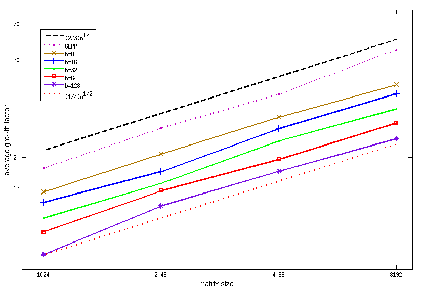
Figure 1: Growth factor $g_{W}$ of the LU_PRRP factorization of random matrices.

Tables 16 and 18 in Appendix B present more detailed results showing the stability of the LU_PRRP factorization for random matrices and a set of special matrices. There, we include different metrics, such as the norm of the factors, the value of their maximum element and the backward error of the LU factorization. We evaluate the normwise backward stability by computing three accuracy tests as performed in the HPL (High-Performance Linpack) benchmark [6], and denoted as HPL1, HPL2 and HPL3.

HPL1 $$= ||Ax-b||_{\infty}/(\epsilon||A||_{1}*N),$$

HPL2 $$= ||Ax-b||_{\infty}/(\epsilon||A||_{1}||x||_{1}),$$

HPL3 $$= ||Ax-b||_{\infty}/(\epsilon||A||_{\infty}||x||_{\infty}*N).$$

In HPL, the method is considered to be accurate if the values of the three quantities are smaller than $16$. More generally, the values should be of order $O(1)$. For the LU_PRRP factorization HPL1 is at most $8.09$, HPL2 is at most $8.04\times 10^{-2}$ and HPL3 is at most $1.60\times 10^{-2}$. We also display the normwise backward error, using the 1-norm,

$$\eta:=\frac{||r||}{||A||~{}||x||+||b||},$$ (13)

and the componentwise backward error

$$w:=\max_{i}\frac{|r_{i}|}{(|A|~{}|{x}|+|b|)_{i}},$$ (14)

where the computed residual is $r=b-A{x}$. For our tests residuals are computed with double-working precision.

Figure 2 summarizes all our stability results for LU_PRRP. This figure displays the ratio of the maximum between the backward error and machine epsilon of LU_PRRP versus GEPP. The backward error is measured using three metrics, the relative error $\|PA-LU\|/\|A\|$, the normwise backward error $\eta$, and the componentwise backward error $w$ of LU_PRRP versus GEPP, and the machine epsilon. We take the maximum of the computed error with epsilon since smaller values are mostly roundoff error, and so taking ratios can lead to extreme values with little reliability. Results for all the matrices in our test set are presented, that is $20$ random matrices for which results are presented in Table 16, and $37$ special matrices for which results are presented in Tables 17 and 18. This figure shows that for random matrices, almost all ratios are between $0.5$ and $2$. For special matrices, there are few outliers, up to $23.71$ (GEPP is more stable) for the backward error ratio of the special matrix hadamard and down to $2.12\times 10^{-2}$ (LU_PRRP is more stable) for the backward error ratio of the special matrix moler.

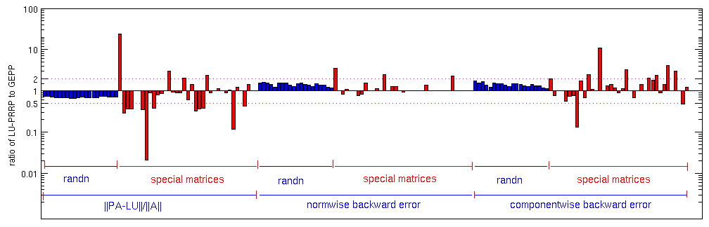
Figure 2: A summary of all our experimental data, showing the ratio between max(LU_PRRP’s backward error, machine epsilon) and max(GEPP’s backward error, machine epsilon) for all the test matrices in our set. Each vertical bar represents such a ratio for one test matrix. Bars above $10^{0}=1$ mean that LU_PRRP’s backward error is larger, and bars below $1$ mean that GEPP’s backward error is larger. For each matrix and algorithm, the backward error is measured 3 ways. For the first third of the bars, labeled $\|PA-LU\|/\|A\|$, the metric is the backward error, using the Frobenius norm. For the middle third of the bars, labeled “normwise backward error”, the metric is $\eta$ in equation (13). For the last third of the bars, labeled “componentwise backward error”, the metric is $w$ in equation (14). The test matrices are further labeled either as “randn”, which are randomly generated, or “special”, listed in Table LABEL:Tab_allTestMatrix.

We consider now pathological matrices on which GEPP fails. Table 2 presents results for the linear solver using the LU_PRRP factorization for a Wilkinson matrix [22] of size $2048$ with a size of the panel varying from $8$ to $128$. The growth factor is 1 and the relative error $\frac{||PA-LU||}{||A||}$ is on the order of $10^{-19}$. Table 3 presents results for the linear solver using the LU_PRRP algorithm for a generalized Wilkinson matrix of size $2048$ with a size of the panel varying from $8$ to $128$.

Table 2: Stability of the LU_PRRP factorization of a Wilkinson matrix on which GEPP fails.

n	b	$g_{W}$	$||U||_{1}$	$||U^{-1}||_{1}$	$||L||_{1}$	$||L^{-1}||_{1}$	$\frac{||PA-LU||_{F}}{||A||_{F}}$
2048	128	1	1.02e+03	6.09e+00	1	1.95e+00	4.25e-20
	64	1	1.02e+03	6.09e+00	1	1.95e+00	5.29e-20
	32	1	1.02e+03	6.09e+00	1	1.95e+00	8.63e-20
	16	1	1.02e+03	6.09e+00	1	1.95e+00	1.13e-19
	8	1	1.02e+03	6.09e+00	1	1.95e+00	1.57e-19

Table 3: Stability of the LU_PRRP factorization of a generalized Wilkinson matrix on which GEPP fails.

n	b	$g_{W}$	$||U||_{1}$	$||U^{-1}||_{1}$	$||L||_{1}$	$||L^{-1}||_{1}$	$\frac{||PA-LU||_{F}}{||A||_{F}}$
2048	128	2.69	1.23e+03	1.39e+02	1.21e+03	1.17e+03	1.05e-15
	64	2.61	9.09e+02	1.12e+02	1.36e+03	1.15e+03	9.43e-16
	32	2.41	8.20e+02	1.28e+02	1.39e+03	9.77e+02	5.53e-16
	16	4.08	1.27e+03	2.79e+02	1.41e+03	1.19e+03	7.92e-16
	8	3.35	1.36e+03	2.19e+02	1.41e+03	1.73e+03	1.02e-15

For the Foster matrix, it was shown that when $c=1$ and $kh={2\over 3}$, the growth factor of GEPP is $({2\over 3})(2^{n-1}-1)$, which is close to the maximum theoretical growth factor of GEPP of $2^{n-1}$. Table 4 presents results for the linear solver using the LU_PRRP factorization for a Foster matrix of size $2048$ with a size of the panel varying from $8$ to $128$ ( $c=1$, $h=1$ and $k={2\over 3}$ ). According to the obtained results, LU_PRRP gives a modest growth factor of $2.66$ for this practical matrix, while GEPP has a growth factor of $10^{18}$ for the same parameters.

Table 4: Stability of the LU_PRRP factorization of a practical matrix (Foster) on which GEPP fails.

n	b	$g_{W}$	$||U||_{1}$	$||U^{-1}||_{1}$	$||L||_{1}$	$||L^{-1}||_{1}$	$\frac{||PA-LU||_{F}}{||A||_{F}}$
2048	128	2.66	1.28e+03	1.87e+00	1.92e+03	1.92e+03	4.67e-16
	64	2.66	1.19e+03	1.87e+00	1.98e+03	1.79e+03	2.64e-16
	32	2.66	4.33e+01	1.87e+00	2.01e+03	3.30e+01	2.83e-16
	16	2.66	1.35e+03	1.87e+00	2.03e+03	2.03e+00	2.38e-16
	8	2.66	1.35e+03	1.87e+00	2.04e+03	2.02e+00	5.36e-17

For matrices arising from the two-point boundary value problems described by Wright, it was shown that when $h$ is chosen small enough such that all elements of $e^{Mh}$ are less than 1 in magnitude, the growth factor obtained using GEPP is exponential. For our experiment the matrix $M=\left[\begin{array}[]{cc}-{1\over 6}&1\\ 1&-{1\over 6}\\ \end{array}\right]$, that is $e^{Mh}\approx\left[\begin{array}[]{cc}1-{h\over 6}&h\\ h&1-{h\over 6}\\ \end{array}\right]$, and $h=0.3$. Table 5 presents results for the linear solver using the LU_PRRP factorization for a Wright matrix of size $2048$ with a size of the panel varying from $8$ to $128$. According to the obtained results, again LU_PRRP gives minimum possible pivot growth $1$ for this practical matrix, compared to the GEPP method which leads to a growth factor of $10^{95}$ using the same parameters.

Table 5: Stability of the LU_PRRP factorization on a practical matrix (Wright) on which GEPP fails.

n	b	$g_{W}$	$||U||_{1}$	$||U^{-1}||_{1}$	$||L||_{1}$	$||L^{-1}||_{1}$	$\frac{||PA-LU||_{F}}{||A||_{F}}$
2048	128	1	3.25e+00	8.00e+00	2.00e+00	2.00e+00	4.08e-17
	64	1	3.25e+00	8.00e+00	2.00e+00	2.00e+00	4.08e-17
	32	1	3.25e+00	8.00e+00	2.05e+00	2.07e+00	6.65e-17
	16	1	3.25e+00	8.00e+00	2.32e+00	2.44e+00	1.04e-16
	8	1	3.40e+00	8.00e+00	2.62e+00	3.65e+00	1.26e-16

All the previous tests show that the LU_PRRP factorization is very stable for random, and for more special matrices, and it also gives modest growth factor for the pathological matrices on which GEPP fails. We note that we were not able to find matrices for which LU_PRRP attains the upper bound of ${\displaystyle(1+\tau b)^{n\over b}}$ for the growth factor.

3 Communication avoiding LU_PRRP

In this section we present a communication avoiding version of the LU_PRRP algorithm, that is an algorithm that minimizes communication, and so it will be more efficient than LU_PRRP and GEPP on architectures where communication is expensive. We show in this section that this algorithm is more stable than CALU, an existing communication avoiding algorithm for computing the LU factorization [10]. More importantly, its parallel version is also more stable than GEPP (under certain conditions).

3.1 Matrix algebra

CALU_PRRP is a block algorithm that uses tournament pivoting, a strategy introduced in [10] that allows to minimize communication. As in LU_PRRP, at each step the factorization of the current panel is computed, and then the trailing matrix is updated. However, in CALU_PRRP the panel factorization is performed in two steps. The first step, which is a preprocessing step, uses a reduction operation to identify $b$ pivot rows with a minimum amount of communication. The strong RRQR factorization is the operator used at each node of the reduction tree to select a new set of $b$ candidate rows from the candidate rows selected at previous stages of the reduction. The $b$ pivot rows are permuted into the diagonal positions, and then the QR factorization with no pivoting of the transpose of the entire panel is computed.

In the following we illustrate tournament pivoting on the first panel, with the input matrix $A$ partitioned as in equation (3). Tournament pivoting considers that the first panel is partitioned into $P=4$ blocks of rows,

$$A(:,1:b)=\left[\begin{array}[]{c}A_{00}\\ A_{10}\\ A_{20}\\ A_{30}\\ \end{array}\right].$$

The preprocessing step uses a binary reduction tree in our example, and we number the levels of the reduction tree starting from $0$. At the leaves of the reduction tree, a set of $b$ candidate rows are selected from each block of rows $A_{i0}$ by performing the strong RRQR factorization on the transpose of each block $A_{i0}$. This gives the following decomposition,

$$\left[\begin{array}[]{c}A_{00}^{T}\Pi_{00}\\ A_{10}^{T}\Pi_{10}\\ A_{20}^{T}\Pi_{20}\\ A_{30}^{T}\Pi_{30}\\ \end{array}\right]=\left[\begin{array}[]{c}Q_{00}R_{00}\\ Q_{10}R_{10}\\ Q_{20}R_{20}\\ Q_{30}R_{30}\\ \end{array}\right],$$

which can be written as

$$A(:,1:b)^{T}\bar{\Pi}_{0}=A(:,1:b)^{T}\left[\begin{array}[]{cccc}\Pi_{00}&&&\\ &\Pi_{10}&&\\ &&\Pi_{20}&\\ &&&\Pi_{30}\\ \end{array}\right] = \left[\begin{array}[]{c}Q_{00}R_{00}\\ Q_{10}R_{10}\\ Q_{20}R_{20}\\ Q_{30}R_{30}\\ \end{array}\right],$$

where $\bar{\Pi}_{0}$ is an $m\times m$ permutation matrix with diagonal blocks of size ${m\over P}\times{m\over P}$, $Q_{i0}$ is an orthogonal matrix of size $b\times b$, and each factor $R_{i0}$ is an $b\times{m\over P}$ upper triangular matrix.

There are now $P=4$ sets of candidate rows. At the first level of the binary tree, two matrices $A_{01}$ and $A_{11}$ are formed by combining together two sets of candidate rows,

$$A_{01} = \left[\begin{array}[]{c}(A_{00}^{T}\Pi_{00})(:,1:b)\\ (A_{10}^{T}\Pi_{10})(:,1:b)\end{array}\right]$$

$$A_{11} = \left[\begin{array}[]{c}(A_{20}^{T}\Pi_{20})(:,1:b)\\ (A_{30}^{T}\Pi_{30})(:,1:b)\end{array}\right].$$

Two new sets of candidate rows are identified by performing the strong RRQR factorization of each matrix $A_{01}$ and $A_{11}$,

$$A_{01}^{T}\Pi_{01}=Q_{01}R_{01},$$

$$A_{11}^{T}\Pi_{11}=Q_{11}R_{11},$$

where $\Pi_{10}$, $\Pi_{11}$ are permutation matrices of size $2b\times 2b$, $Q_{01}$, $Q_{11}$ are orthogonal matrices of size $b\times b$, and $R_{01},R_{11}$ are upper triangular factors of size $b\times 2b$.

The final $b$ pivot rows are obtained by performing one last strong RRQR factorization on the transpose of the following $b\times 2b$ matrix :

$$A_{02}=\left[\begin{array}[]{c}(A_{01}^{T}\Pi_{01})(:,1:b)\\ (A_{11}^{T}\Pi_{11})(:,1:b)\end{array}\right],$$

that is

$$A_{02}^{T}\Pi_{02}=Q_{02}R_{02},$$

where $\Pi_{02}$ is a permutation matrix of size $2b\times 2b$, $Q_{02}$ is an orthogonal matrix of size $b\times b$, and $R_{02}$ is an upper triangular matrix of size $b\times 2b$. This operation is performed at the root of the binary reduction tree, and this ends the first step of the panel factorization. In the second step, the final pivot rows identified by tournament pivoting are permuted to the diagonal positions of $A$,

$${\hat{A}}=\bar{\Pi}^{T}A=\bar{\Pi}_{2}^{T}\bar{\Pi}_{1}^{T}\bar{\Pi}_{0}^{T}A,$$

where the matrices $\bar{\Pi}_{i}$ are obtained by extending the matrices $\bar{\Pi}$ to the dimension $m\times m$, that is

$$\bar{\Pi}_{1}=\left[\begin{array}[]{cc}\bar{\Pi}_{01}&\\ &\bar{\Pi}_{11}\\ \end{array}\right],$$

with $\bar{\Pi}_{i1}$, for $i=0,1$ formed as

$$\bar{\Pi}_{i1}=\left[\begin{array}[]{cccc}\Pi_{i1}(1:b,1:b)&&\Pi_{i1}(1:b,b+1:2b)&\\ &I_{{m\over P}-b}&&\\ \Pi_{i1}(b+1:2b,1:b)&&\Pi_{i1}(b+1:2b,b+1:2b)&\\ &&&I_{{m\over P}-b}\\ \end{array}\right],$$

and

$$\bar{\Pi}_{2}=\left[\begin{array}[]{cccc}\Pi_{02}(1:b,1:b)&&\Pi_{02}(1:b,b+1:2b)&\\ &I_{2{m\over P}-b}&&\\ \Pi_{02}(b+1:2b,1:b)&&\Pi_{02}(b+1:2b,b+1:2b)&\\ &&&I_{2{m\over P}-b}\\ \end{array}\right].$$

Once the pivot rows are in the diagonal positions, the QR factorization with no pivoting is performed on the transpose of the first panel,

$${\hat{A}}^{T}(1:b,:)=QR=\left[\begin{array}[]{cc}R_{11}&R_{12}\end{array}\right].$$

This factorization is used to update the trailing matrix, and the elimination of the first panel leads to the following decomposition (we use the same notation as in section 2),

$${\hat{A}}=\left[\begin{array}[]{cc}I_{b}&\\ {\hat{A}}_{21}{{\hat{A}}_{11}}^{-1}&I_{m-b}\\ \end{array}\right]\left[\begin{array}[]{cc}{\hat{A}}_{11}&{\hat{A}}_{12}\\ &{{\hat{A}}}_{22}^{s}\\ \end{array}\right],$$

where

$${{\hat{A}}}_{22}^{s}={\hat{A}}_{22}-{\hat{A}}_{21}{{\hat{A}}_{11}}^{-1}{\hat{A}}_{12}.$$

As in the LU_PRRP factorization, the CALU_PRRP factorization computes a block LU factorization of the input matrix $A$. To obtain the full LU factorization, an additional GEPP is performed on the diagonal block ${\hat{A}}_{11}$, followed by the update of the block row ${\hat{A}}_{12}$. The CALU_PRRP factorization continues the same procedure on the trailing matrix ${{\hat{A}}}_{22}^{s}$.

Note that the factors $L$ and $U$ obtained by the CALU_PRRP factorization are different from the factors obtained by the LU_PRRP factorization. The two algorithms use different pivot rows, and in particular the factor $L$ of CALU_PRRP is no longer bounded by a given threshold $\tau$ as in LU_PRRP. This leads to a different worst case growth factor for CALU_PRRP, that we will discuss in the following section.

The following figure displays the binary tree based tournament pivoting performed on the first panel using an arrow notation (as in [10]). The function $f(A_{ij})$ computes a strong RRQR of the matrix $A^{T}_{ij}$ to select a set of $b$ candidate rows. At each node of the reduction tree, two sets of $b$ candidate rows are merged together and form a matrix $A_{ij}$, the function $f$ is applied on $A_{ij}$, and another set of $b$ candidate rows is selected. While in this section we focused on binary trees, tournament pivoting can use any reduction tree, and this allows the algorithm to adapt on different architectures. Later in the paper we will consider also a flat reduction tree.

3.2 Numerical Stability of CALU_PRRP

In this section we discuss the stability of the CALU_PRRP factorization and we identify similarities with the LU_PRRP factorization. We also discuss the growth factor of the CALU_PRRP factorization, and we show that its upper bound depends on the height of the reduction tree. For the same reduction tree, this upper bound is smaller than that obtained with CALU. More importantly, for cases of interest, the upper bound of the growth factor of CALU_PRRP is also smaller than that obtained with GEPP.

To address the numerical stability of CALU_PRRP, we show that performing CALU_PRRP on a matrix $A$ is equivalent to performing LU_PRRP on a larger matrix $A_{{{LU\_PRRP}}}$, which is formed by blocks of $A$ (sometimes slightly perturbed) and blocks of zeros. This reasoning is also used in [10] to show the same equivalence between CALU and GEPP. While this similarity is explained in detail in [10], here we focus only on the first step of the CALU_PRRP factorization. We explain the construction of the larger matrix $A_{{{LU\_PRRP}}}$ to expose the equivalence between the first step of the CALU_PRRP factorization of $A$ and the LU_PRRP factorization of $A_{{{LU\_PRRP}}}$.

Consider a nonsingular matrix $A$ of size $m\times n$ and the first step of its CALU_PRRP factorization using a general reduction tree of height $H$. Tournament pivoting selects $b$ candidate rows at each node of the reduction tree by using the strong RRQR factorization. Each such factorization leads to an $L$ factor which is bounded locally by a given threshold $\tau$. However this bound is not guaranteed globally. When the factorization of the first panel is computed using the $b$ pivot rows selected by tournament pivoting, the $L$ factor will not be bounded by $\tau$. This results in a larger growth factor than the one obtained with the LU_PRRP factorization. Recall that in LU_PRRP, the strong RRQR factorization is performed on the transpose of the whole panel, and so every entry of the obtained lower triangular factor $L$ is bounded by $\tau$.

However, we show now that the growth factor obtained after the first step of the CALU_PRRP factorization is bounded by $(1+\tau b)^{H+1}$. Consider a row $j$, and let $A^{s}(j,b+1:n)$ be the updated row obtained after the first step of elimination of CALU_PRRP. Suppose that row $j$ of $A$ is a candidate row at level $k-1$ of the reduction tree, and so it participates in the strong RRQR factorization computed at a node $s_{k}$ at level $k$ of the reduction tree, but it is not selected as a candidate row by this factorization. We refer to the matrix formed by the candidate rows at node $s_{k}$ as ${\bar{A}}_{k}$. Hence, row $j$ is not used to form the matrix ${\bar{A}}_{k}$. Similarly, for every node $i$ on the path from node $s_{k}$ to the root of the reduction tree of height $H$, we refer to the matrix formed by the candidate rows selected by strong RRQR as ${\bar{A}}_{i}$. Note that in practice it can happen that one of the blocks of the panel is singular, while the entire panel is nonsingular. In this case strong RRQR will select less than $b$ linearly independent rows that will be passed along the reduction tree. However, for simplicity, we assume in the following that the matrices ${\bar{A}}_{i}$ are nonsingular. For a more general solution, the reader can consult [10].

Let $\Pi$ be the permutation returned by the tournament pivoting strategy performed on the first panel, that is the permutation that puts the matrix ${\bar{A}}_{H}$ on diagonal. The following equation is satisfied,

$$\begin{pmatrix}{\bar{A}}_{H}&{\hat{A}}_{H}\\ A(j,1:b)&A(j,b+1:n)\\ \end{pmatrix}=\begin{pmatrix}I_{b}&\\ A(j,1:b){\bar{A}}_{H}^{-1}&1\\ \end{pmatrix}\cdot\begin{pmatrix}{\bar{A}}_{H}&{\hat{A}}_{H}\\ &A^{s}(j,b+1:n)\end{pmatrix},$$ (25)

where

$${\bar{A}}_{H} = (\Pi A)(1:b,1:b),$$

$${\hat{A}}_{H} = (\Pi A)(1:b,b+1:n).$$

The updated row $A^{s}(j,b+1:n)$ can be also obtained by performing LU_PRRP on a larger matrix $A_{{{LU\_PRRP}}}$ of dimension $((H-k+1)b+1)\times((H-k+1)b+1)$,

$$A_{{{LU\_PRRP}}} = \begin{pmatrix}{\bar{A}}_{H}&&&&&{\hat{A}}_{H}\\ {\bar{A}}_{H-1}&{\bar{A}}_{H-1}&&&&\\ &{\bar{A}}_{H-2}&{\bar{A}}_{H-2}&&&\\ &&\ddots&\ddots&&\\ &&&{\bar{A}}_{k}&{\bar{A}}_{k}&\\ &&&&(-1)^{H-k}A(j,1:b)&A(j,b+1:n)\\ \end{pmatrix}$$ (26)

$$= \begin{pmatrix}I_{b}&&&&&\\ {\bar{A}}_{H-1}{\bar{A}}_{H}^{-1}&I_{b}&&&&\\ &{\bar{A}}_{H-2}{\bar{A}}_{H-1}^{-1}&I_{b}&&&\\ &&\ddots&\ddots&&\\ &&&{\bar{A}}_{k}{\bar{A}}_{k+1}^{-1}&I_{b}&\\ &&&&(-1)^{H-k}A(j,1:b){\bar{A}}_{k}^{-1}&1\\ \end{pmatrix}$$

$$\cdot \begin{pmatrix}{\bar{A}}_{H}&&&&&{\hat{A}}_{H}\\ &{\bar{A}}_{H-1}&&&&{\hat{A}}_{H-1}\\ &&{\bar{A}}_{H-2}&&&{\hat{A}}_{H-2}\\ &&&\ddots&&\vdots\\ &&&&{\bar{A}}_{k}&{\hat{A}}_{k}\\ &&&&&A^{s}(j,b+1:n)\\ \end{pmatrix},$$

where

$${\hat{A}}_{H-i} = \left\{\begin{array}[]{ll}{\bar{A}}_{H}&{\rm if}\;i=0,\\ -{\bar{A}}_{H-i}{\bar{A}}_{H-i+1}^{-1}{\hat{A}}_{H-i+1}&{\rm if}\;0<i\leq H-k.\\ \end{array}\right.$$ (29)

Equation (26) can be easily verified, since

$$A^{s}(j,b+1:n) = A(j,b+1:n)-(-1)^{H-k}A(j,1:b){\bar{A}}_{k}^{-1}(-1)^{H-k}{\hat{A}}_{k}$$

$$= A(j,b+1:n)-A(j,1:b){\bar{A}}_{k}^{-1}{\bar{A}}_{k}{\bar{A}}_{k+1}^{-1}\ldots{\bar{A}}_{H-2}{\bar{A}}_{H-1}^{-1}{\bar{A}}_{H-1}{\bar{A}}_{H}^{-1}{\hat{A}}_{H}$$

$$= A(j,b+1:n)-A(j,1:b){\bar{A}}_{H}^{-1}{\hat{A}}_{H}.$$

Equations (25) and (26) show that the Schur complement obtained after each step of performing the CALU_PRRP factorization of a matrix $A$ is equivalent to the Schur complement obtained after performing the LU_PRRP factorization of a larger matrix $A_{LU\_PRRP}$, formed by blocks of $A$ (sometimes slightly perturbed) and blocks of zeros. More generally, this implies that the entire CALU_PRRP factorization of $A$ is equivalent to the LU_PRRP factorization of a larger and very sparse matrix, formed by blocks of $A$ and blocks of zeros (we omit the proofs here, since they are similar with the proofs presented in [10]).

Equation (26) is used to derive the upper bound of the growth factor of CALU_PRRP from the upper bound of the growth factor of LU_PRRP. The elimination of each row of the first panel using CALU_PRRP can be obtained by performing LU_PRRP on a matrix of maximum dimension $m\times b(H+1)$. Hence the upper bound of the growth factor obtained after one step of CALU_PRRP is $(1+\tau b)^{H+1}$. This leads to an upper bound of $(1+\tau b)^{{n\over b}(H+1)-1}$ for a matrix of size $m\times n$.

Table 6 summarizes the bounds of the growth factor of CALU_PRRP derived in this section, and also recalls the bounds of LU_PRRP, GEPP, and CALU the communication avoiding version of GEPP. It considers the growth factor obtained after the elimination of $b$ columns of a matrix of size $m\times(b+1)$, and also the general case of a matrix of size $m\times n$. As discussed in section 2 already, LU_PRRP is more stable than GEPP in terms of worst case growth factor. From Table 6, it can be seen that for a reduction tree of a same height, CALU_PRRP is more stable than CALU.

In the following we show that CALU_PRRP can be more stable than GEPP in terms of worst case growth factor. Consider a parallel version of CALU_PRRP based on a binary reduction tree of height $H=\log(P)$, where $P$ is the number of processors. The upper bound of the growth factor becomes $(1+\tau b)^{{{n(logP+1)}\over{b}}-1}$, which is smaller than $2^{n(logP+1)-1}$, the upper bound of the growth factor of CALU. For example, if the threshold is $\tau=2$, the panel size is $b=64$, and the number of processors is $P=128=2^{7}$, then ${g_{W}}_{{{CALU\_PRRP}}}=(1.7)^{n}$. This quantity is much smaller than $2^{7n}$ the upper bound of CALU, and even smaller than the worst case growth factor of GEPP of $2^{n-1}$. In general, the upper bound of CALU_PRRP can be smaller than the one of GEPP, if the different parameters $\tau$, $H$, and $b$ are chosen such that the condition

$$H\leq{b\over(\log b+\log\tau)}$$ (30)

is satisfied. For a binary tree of height $H=\log P$, it becomes $\log P\leq{b\over(\log b+\log\tau)}$. This is a condition which can be satisfied in practice, by choosing $b$ and $\tau$ appropriately for a given number of processors $P$. For example, when $P\leq 512$, $b=64$, and $\tau=2$, the condition (30) is satisfied, and the worst case growth factor of CALU_PRRP is smaller than the one of GEPP.

However, for a sequential version of CALU_PRRP using a flat tree of height $H=n/b$, the condition to be satisfied becomes $n\leq{b^{2}\over(\log b+\log\tau)}$, which is more restrictive. In practice, the size of $b$ is chosen depending on the size of the memory, and it might be the case that it will not satisfy the condition in equation (30).

Table 6: Bounds for the growth factor $g_{W}$ obtained from factoring a matrix of size $m\times(b+1)$ and a matrix of size $m\times n$ using CALU_PRRP, LU_PRRP, CALU, and GEPP. CALU_PRRP and CALU use a reduction tree of height $H$. The strong RRQR used in LU_PRRP and CALU_PRRP is based on a threshold $\tau$. For the matrix of size $m\times(b+1)$, the result corresponds to the growth factor obtained after eliminating $b$ columns.

	matrix of size $m\times(b+1)$
	TSLU(b,H)	LU_PRRP(b,H)	GEPP	LU_PRRP
$g_{W}$ upper bound	$2^{b(H+1)}$	$(1+\tau b)^{{H+1}}$	$2^{b}$	$1+\tau b$
	matrix of size $m\times n$
	CALU	CALU_PRRP	GEPP	LU_PRRP
$g_{W}$ upper bound	$2^{n(H+1)-1}$	$(1+\tau b)^{{{n(H+1)}\over{b}}-1}$	$2^{n-1}$	$(1+\tau b)^{n\over b}$

3.3 Experimental results

In this section we present experimental results and show that CALU_PRRP is stable in practice and compare them with those obtained from CALU and GEPP in [10]. We present results for both the binary tree scheme and the flat tree scheme.

As in section 2, we perform our tests on matrices whose elements follow a normal distribution. In Matlab notation, the test matrix is $A={\sf randn}(n,n)$, and the right hand side is $b={\sf randn}(n,1)$. The size of the matrix is chosen such that $n$ is a power of $2$, that is $n=2^{k}$, and the sample size is 10 if $k<13$ and 3 if $k\geq 13$. To measure the stability of CALU_PRRP, we discuss several metrics, that concern the LU decomposition and the linear solver using it, such as the growth factor, normwise and componentwise backward errors. We also perform tests on several special matrices including sparse matrices, they are described in Appendix B.

Figure 3 displays the values of the growth factor $g_{W}$ of the binary tree based CALU_PRRP, for different block sizes $b$ and different number of processors $P$. As explained in section 3.1, the block size determines the size of the panel, while the number of processors determines the number of block rows in which the panel is partitioned. This corresponds to the number of leaves of the binary tree. We observe that the growth factor of binary tree based CALU_PRRP is in the most of the cases better than GEPP. The curves of the growth factor lie between ${1\over 2}n^{1/2}$ and ${3\over 4}n^{1/2}$ in our tests on random matrices. These results show that binary tree based CALU_PRRP is stable and the growth factor values obtained for the different layouts are better than those obtained with binary tree based CALU. The figure 3 includes also the growth factor of the LU_PRRP method with a panel of size $b=64$. We note that that results are better than those of binary tree based CALU_PRRP.

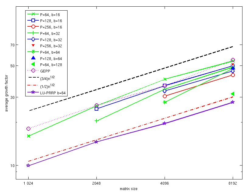
Figure 3: Growth factor $g_{W}$ of binary tree based CALU_PRRP for random matrices.

Figure 4 displays the values of the growth factor $g_{W}$ for flat tree based CALU_PRRP with a block size $b$ varying from $8$ to $128$. The growth factor $g_{W}$ is decreasing with increasing the panel size b. We note that the curves of the growth factor lie between ${1\over 4}n^{1/2}$ and ${3\over 4}n^{1/2}$ in our tests on random matrices. We also note that the results obtained with the LU_PRRP method with a panel of size $b=64$ are better than those of flat tree based CALU_PRRP.

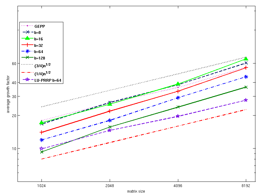
Figure 4: Growth factor $g_{W}$ of flat tree based CALU_PRRP for random matrices.

The growth factors of both binary tree based and flat tree based CALU_PRRP have similar (sometimes better) behavior than the growth factors of GEPP.

Table 19 in Appendix B presents results for the linear solver using binary tree based CALU_PRRP, together with binary tree based CALU and GEPP for comparaison and Table 20 in Appendix B presents results for the linear solver using flat tree based CALU_PRRP, together with flat tree based CALU and GEPP for comparaison. We note that for the binary tree based CALU_PRRP, when ${m\over P}=b$, for the algorithm we only use $P1={m\over(b+1)}$ processors, since to perform a Strong RRQR on a given block, the number of its rows should be at least the number of its columns $+1$. Tables 19 and 20 also include results obtained by iterative refinement used to improve the accuracy of the solution. For this, the componentwise backward error in equation (14) is used. In the previous tables, $w_{b}$ denotes the componentwise backward error before iterative refinement and $N_{IR}$ denotes the number of steps of iterative refinement. $N_{IR}$ is not always an integer since it represents an average. For all the matrices tested CALU_PRRP leads to results as accurate as the results obtained with CALU and GEPP.

In Appendix B we present more detailed results. There we include some other metrics, such as the norm of the factors, the norm of the inverse of the factors, their conditioning, the value of their maximum element, and the backward error of the LU factorization. Through the results detailed in this section and in Appendix B we show that binary tree based and flat tree based CALU_PRRP are stable, have the same behavior as GEPP for random matrices, and are more stable than binary tree based and flat tree based CALU in terms of growth factor.

Figure 5 summarizes all our stability results for the CALU_PRRP factorization based on both binary tree and flat tree schemes. As figure 2, this figure displays the ratio of the maximum between the backward error and machine epsilon of LU_PRRP versus GEPP. The backward error is measured as the relative error $\|PA-LU\|/\|A\|$, the normwise backward error $\eta$, and the componentwise backward error $w$. Results for all the matrices in our test set are presented, that is $25$ random matrices for binary tree base CALU_PRRP from Table 23, $20$ random matrices for flat tree based CALU_PRRP from Table 21, and $37$ special matrices from Tables 22 and 24. As it can be seen, nearly all ratios are between $0.5$ and $2.5$ for random matrices. However there are few outliers, for example the relative error ratio has values between $24.2$ for the special matrix hadamard (GEPP is more stable than binary tree based CALU_PRRP), and $5.8\times 10^{-3}$ for the special matrix moler (binary tree based CALU_PRRP is more stable than GEPP).

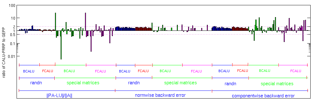
Figure 5: A summary of all our experimental data, showing the ratio of max(CALU_PRRP’s backward error, machine epsilon) to max(GEPP’s backward error, machine epsilon) for all the test matrices in our set. Each vertical bar represents such a ratio for one test matrix. Bars above $10^{0}=1$ mean that CALU_PRRP’s backward error is larger, and bars below $1$ mean that GEPP’s backward error is larger. For each matrix and algorithm, the backward error is measured using three different metrics. For the last third of the bars, labeled “componentwise backward error”, the metric is $w$ in equation (14). The test matrices are further labeled either as “randn”, which are randomly generated, or “special”, listed in Table LABEL:Tab_allTestMatrix. Finally, each test matrix is factored using CALU_PRRP with a binary reduction tree (labeled BCALU for BCALU_PRRP) and with a flat reduction tree (labeled FCALU for FCALU_PRRP).

We consider now the same set of pathological matrices as in section 2 on which GEPP fails. For the Wilkinson matrix, both CALU and CALU_PRRP based on flat and binary tree give modest element growth. For the generalized Wilkinson matrix, the Foster matrix, and Wright matrix, CALU fails with both flat tree and binary tree reduction schemes.

Tables 7 and 8 present the results obtained for the linear solver using the CALU_PRRP factorization based on flat and binary tree schemes for a generalized Wilkinson matrix of size $2048$ with a size of the panel varying from $8$ to $128$ for the flat tree scheme and a number of processors varying from $128$ to $32$ for the binary tree scheme. The growth factor is of order 1 and the quantity $\frac{||PA-LU||}{||A||}$ is on the order of $10^{-16}$. Both flat tree based CALU and binary tree based CALU fail on this pathological matrix. In fact for a generalized Wilkinson matrix of size $1024$ and a panel of size $b=128$, the growth factor obtained with flat tree based CALU is of size $10^{234}$.

Table 7: Stability of the flat tree based CALU_PRRP factorization of a generalized Wilkinson matrix on which GEPP fails.

n	b	$g_{W}$	$||U||_{1}$	$||U^{-1}||_{1}$	$||L||_{1}$	$||L^{-1}||_{1}$	$\frac{||PA-LU||_{F}}{||A||_{F}}$
2048	128	2.01	1.01e+03	1.40e+02	1.31e+03	9.76e+02	9.56e-16
	64	2.02	1.18e+03	1.64e+02	1.27e+03	1.16e+03	1.01e-15
	32	2.04	8.34e+02	1.60e+02	1.30e+03	7.44e+02	7.91e-16
	16	2.15	9.10e+02	1.45e+02	1.31e+03	8.22e+02	8.07e-16
	8	2.15	8.71e+02	1.57e+02	1.371e+03	5.46e+02	6.09e-16

Table 8: Stability of the binary tree based CALU_PRRP factorization of a generalized Wilkinson matrix on which GEPP fails.

n	P	b	$g_{W}$	$||U||_{1}$	$||U^{-1}||_{1}$	$||L||_{1}$	$||L^{-1}||_{1}$	$\frac{||PA-LU||_{F}}{||A||_{F}}$
2048	128	8	2.10e+00	1.33e+03	1.29e+02	1.34e+03	1.33e+03	1.08e-15
	64	16	2.04e+00	6.85e+02	1.30e+02	1.30e+03	6.85e+02	7.85e-16
		8	8.78e+01	1.21e+03	1.60e+02	1.33e+03	1.01e+03	9.54e-16
	32	32	2.08e+00	9.47e+02	1.58e+02	1.41e+03	9.36e+02	5.95e-16
		16	2.08e+00	1.24e+03	1.32e+02	1.35e+03	1.24e+03	1.01e-15
		8	1.45e+02	1.03e+03	1.54e+02	1.37e+03	6.61e+02	6.91e-16

For the Foster matrix, we have seen in the section 2 that LU_PRRP gives modest pivot growth, whereas GEPP fails. Both flat tree based CALU and binary tree based CALU fail on the Foster matrix. However flat tree based CALU_PRRP and binary tree based CALU_PRRP solve easily this pathological matrix.

Tables 9 and 10 present results for the linear solver using the CALU_PRRP factorization based on the flat tree scheme and the binary tree scheme, respectively. We test a Foster matrix of size $2048$ with a panel size varying from $8$ to $128$ for the flat tree based CALU_PRRP and a number of processors varying from $128$ to $32$ for the binary tree based CALU_PRRP. We use the same parameters as in section 2, that is $c=1$, $h=1$ and $k={2\over 3}$. According to the obtained results, CALU_PRRP gives a modest growth factor of $1.33$ for this practical matrix.

Table 9: Stability of the flat tree based CALU_PRRP factorization of a practical matrix (Foster) on which GEPP fails.

n	b	$g_{W}$	$||U||_{1}$	$||U^{-1}||_{1}$	$||L||_{1}$	$||L^{-1}||_{1}$	$\frac{||PA-LU||_{F}}{||A||_{F}}$
2048	128	1.33	1.71e+02	1.87e+00	1.92e+03	1.29e+02	6.51e-17
	64	1.33	8.60e+01	1.87e+00	1.98e+03	6.50e+01	4.87e-17
	32	1.33	4.33e+01	1.87e+00	2.01e+03	3.30e+01	2.91e-17
	16	1.33	2.20e+01	1.87e+00	2.03e+03	1.70e+01	4.80e-17
	8	1.33	1.13e+01	1.87e+00	2.04e+03	9.00e+00	6.07e-17

Table 10: Stability of the binary tree based CALU_PRRP factorization of a practical matrix (Foster) on which GEPP fails.

n	P	b	$g_{W}$	$||U||_{1}$	$||U^{-1}||_{1}$	$||L||_{1}$	$||L^{-1}||_{1}$	$\frac{||PA-LU||_{F}}{||A||_{F}}$
2048	128	8	1.33	1.13e+01	1.87e+00	2.04e+03	9.00e+00	6.07e-17
	64	16	1.33	2.20e+01	1.87e+00	2.03e+03	1.70e+01	4.80e-17
		8	1.33	1.13e+01	1.87e+00	2.04e+03	9.00e+00	6.07e-17
	32	32	1.33	4.33e+01	1.87e+00	2.01e+03	3.300e+01	2.91e-17
		16	1.33	2.20e+01	1.87e+00	2.03e+03	1.70e+01	4.80e-17
		8	1.33	1.13e+01	1.87e+00	2.04e+03	9.00e+00	6.07e-17

As GEPP, both the flat tree based and the binary tree based CALU fail on the Wright matrix. In fact for a matrix of size $2048$, a parameter $h=0.3$, with a panel of size $b=128$, the flat tree based CALU gives a growth factor of $10^{98}$. With a number of processors $P=64$ and a panel of size $b=16$, the binary tree based CALU also gives a growth factor of $10^{98}$. Tables 11 and 12 present results for the linear solver using the CALU_PRRP factorization for a Wright matrix of size $2048$. For the flat tree based CALU_PRRP, the size of the panel is varying from $8$ to $128$. For the binary tree based CALU_PRRP, the number of processors is varying from $32$ to $128$ and the size of the panel from $16$ to $64$ such that the number of rows in the leaf nodes is equal or bigger than two times the size of the panel. The obtained results, show that CALU_PRRP gives a modest growth factor of $1$ for this practical matrix, compared to the CALU method.

Table 11: Stability of the flat tree based CALU_PRRP factorization of a practical matrix (Wright) on which GEPP fails.

n	b	$g_{W}$	$||U||_{1}$	$||U^{-1}||_{1}$	$||L||_{1}$	$||L^{-1}||_{1}$	$\frac{||PA-LU||_{F}}{||A||_{F}}$
2048	128	1	3.25e+00	8.00e+00	2.00e+00	2.00e+00	4.08e-17
	64	1	3.25e+00	8.00e+00	2.00e+00	2.00e+00	4.08e-17
	32	1	3.25e+00	8.00e+00	2.05e+00	2.02e+00	6.65e-17
	16	1	3.25e+00	8.00e+00	2.32e+00	2.18e+00	1.04e-16
	8	1	3.40e+00	8.00e+00	2.62e+00	2.47e+00	1.26e-16

Table 12: Stability of the binary tree based CALU_PRRP factorization of a practical matrix (Wright) on which GEPP fails.

n	P	b	$g_{W}$	$||U||_{1}$	$||U^{-1}||_{1}$	$||L||_{1}$	$||L^{-1}||_{1}$	$\frac{||PA-LU||_{F}}{||A||_{F}}$
2048	128	8	1	3.40e+00	8.00e+00	2.62e+00	2.47e+00	1.26e-16
	64	16	1	3.25e+00	8.00e+00	2.32e+00	2.18e+00	1.04e-16
		8	1	3.40e+00	8.00e+00	2.62e+00	2.47e+00	1.26e-16
	32	32	1	3.25e+00	8.00e+00	2.05e+00	2.02e+00	6.65e-17
		16	1	3.25e+00	8.00e+00	2.32e+00	2.18e+00	1.04e-16
		8	1	3.40e+00	8.00e+00	2.62e+00	2.47e+00	1.26e-16

All the previous tests show that the CALU_PRRP factorization is very stable for random and more special matrices, and it also gives modest growth factor for the pathological matrices on which CALU fails, this is for both binary tree and flat tree based CALU_PRRP.

4 Lower bounds on communication

In this section we focus on the parallel CALU_PRRP algorithm based on a binary reduction tree, and we show that it minimizes the communication between different processors of a parallel computer. For this, we use known lower bounds on the communication performed during the LU factorization of a dense matrix of size $n\times n$, which are

# words_moved $$= \Omega\left(\frac{n^{3}}{\sqrt{M}}\right),$$ (31)

# messages $$= \Omega\left(\frac{n^{3}}{M^{3\over 2}}\right),$$ (32)

where # words_moved refers to the volume of communication, # messages refers to the number of messages exchanged, and $M$ refers to the size of the memory (the fast memory in the case of a sequential algorithm, or the memory per processor in the case of a parallel algorithm). These lower bounds were first introduced for dense matrix multiplication [15], [16], generalized later to LU factorization [4], and then to almost all direct linear algebra [1]. Note that these lower bounds apply to algorithms based on orthogonal transformations under certain conditions [1]. However, this is not relevant to our case, since CALU_PRRP uses orthogonal transformations only to select pivot rows, while the update of the trailing matrix is still performed as in the classic LU factorization algorithm. Hence the lower bounds from equations (31) and, (32) are valid for CALU_PRRP.

We estimate now the cost of computing in parallel the CALU_PRRP factorization of a matrix $A$ of size $m\times n$. The matrix is distributed on a grid of $P=P_{r}\times P_{c}$ processors using a two-dimensional (2D) block cyclic layout. We use the following performance model. Let $\gamma$ be the cost of performing a floating point operation, and let $\alpha+\beta w$ be the cost of sending a message of size $w$ words, where $\alpha$ is the latency cost and $\beta$ is the inverse of the bandwidth. Then, the total running time of an algorithm is estimated to be

$$\alpha\cdot(\text{\# messages})+\beta\cdot(\text{\# words\_moved})+\gamma\cdot(\text{\# flops}),$$

where #messages, #words_moved, and #flops are counted along the critical path of the algorithm.

Table 13 displays the performance of parallel CALU_PRRP (a detailed estimation of the counts is presented in Appendix D). It also recalls the performance of two existing algorithms, the PDGETRF routine from ScaLAPACK which implements GEPP, and the CALU factorization. All three algorithms have the same volume of communication, since it is known that PDGETRF already minimizes the volume of communication. However, the number of messages of both CALU_PRRP and CALU is smaller by a factor of the order of $b$ than the number of messages of PDGETRF. This improvement is achieved thanks to tournament pivoting. In fact, partial pivoting, as used in the routine PDGETRF, leads to an $O(n\log{P})$ number of messages, and because of this, GEPP cannot minimize the number of messages.

Compared to CALU, CALU_PRRP sends a small factor of less messages (depending on $P_{r}$ and $P_{c}$) and performs $\frac{1}{P_{r}}\left(2mn-n^{2}\right)b+\frac{nb^{2}}{3}(5\log_{2}{P_{r}}+1)$ more flops (which represents a lower order term). This is because CALU_PRRP uses the strong RRQR factorization at every node of the reduction tree of every panel factorization, while CALU uses GEPP.

Table 13: Performance estimation of parallel (binary tree based) CALU_PRRP, parallel CALU, and PDGETRF routine when factoring an $m\times n$ matrix, $m\geq n$. The input matrix is distributed using a 2D block cyclic layout on a $P_{r}\times P_{c}$ grid of processors. Some lower order terms are omitted.

	Parallel CALU_PRRP
# messages	$\frac{3n}{b}\log_{2}P_{r}+\frac{2n}{b}\log_{2}{P_{c}}$
# words	$\left(nb+\frac{3}{2}\frac{n^{2}}{P_{c}}\right)\log_{2}P_{r}+\frac{1}{P_{r}}\left(mn-\frac{n^{2}}{2}\right)\log_{2}{P_{c}}$
# flops	$\frac{1}{P}\left(mn^{2}-\frac{n^{3}}{3}\right)+\frac{2}{P_{r}}\left(2mn-n^{2}\right)b+\frac{n^{2}b}{2P_{c}}+\frac{10nb^{2}}{3}\log_{2}{P_{r}}$
	Parallel CALU
# messages	$\frac{3n}{b}\log_{2}P_{r}+\frac{3n}{b}\log_{2}{P_{c}}$
# words	$\left(nb+\frac{3n^{2}}{2P_{c}}\right)\log_{2}P_{r}+\frac{1}{P_{r}}\left(mn-\frac{n^{2}}{2}\right)\log_{2}{P_{c}}$
# flops	$\frac{1}{P}\left(mn^{2}-\frac{n^{3}}{3}\right)+\frac{1}{P_{r}}\left(2mn-n^{2}\right)b+\frac{n^{2}b}{2P_{c}}+\frac{nb^{2}}{3}(5\log_{2}{P_{r}}-1)$
	PDGETRF
# messages	$2n\left(1+\frac{2}{b}\right)\log_{2}{P_{r}}+\frac{3n}{b}\log_{2}{P_{c}}$
# words	$\left(\frac{nb}{2}+\frac{3n^{2}}{2P_{c}}\right)\log_{2}{P_{r}}+\log_{2}{P_{c}}\frac{1}{P_{r}}\left(mn-\frac{n^{2}}{2}\right)$
# flops	$\frac{1}{P}\left(mn^{2}-\frac{n^{3}}{3}\right)+\frac{1}{P_{r}}\left(mn-\frac{n^{2}}{2}\right)b+\frac{n^{2}b}{2P_{c}}$

Despite this additional communication cost, we show now that CALU_PRRP is optimal in terms of communication. We choose optimal values of the parameters $P_{r},P_{c}$, and $b$, as used in CAQR [4] and CALU [10], that is,

$$P_{r}=\sqrt{\frac{mP}{n}}\;\;,\;P_{c}=\sqrt{\frac{nP}{m}}\;\;\text{and}\;b=\frac{1}{4}\log^{-2}\left(\sqrt{\frac{mP}{n}}\right)\cdot\sqrt{\frac{mn}{P}}=\log^{-2}\left(\frac{mP}{n}\right)\cdot\sqrt{\frac{mn}{P}}.$$

For a square matrix of size $n\times n$, the optimal parameters are,

$$P_{r}=\sqrt{P}\;\;,\;P_{c}=\sqrt{P}\;\;\text{and}\;b=\frac{1}{4}\log^{-2}\left(\sqrt{P}\right)\cdot\frac{n}{\sqrt{P}}=\log^{-2}\left(P\right)\cdot\frac{n}{\sqrt{P}}.$$

Table 14 presents the performance estimation of parallel CALU_PRRP and parallel CALU when using the optimal layout. It also recalls the lower bounds on communication from equations (31) and (32) when the size of the memory per processor is on the order of $n^{2}/P$. Both CALU_PRRP and CALU attain the lower bounds on the number of words and on the number of messages, modulo polylogarithmic factors. Note that the optimal layout allows to reduce communication, while keeping the number of extra floating point operations performed due to tournament pivoting as a lower order term. While in this section we focused on minimizing communication between the processors of a parallel computer, it is straightforward to show that the usage of a flat tree during tournament pivoting allows CALU_PRRP to minimize communication between different levels of the memory hierarchy of a sequential computer.

Table 14: Performance estimation of parallel (binary tree based) CALU_PRRP and CALU with an optimal layout. The matrix factored is of size $n\times n$. Some lower-order terms are omitted.

	Parallel CALU_PRRP with optimal layout	Lower bound
# messages	${5\over 2}\sqrt{P}\log^{3}{P}$	$\Omega(\sqrt{P})$
# words	$\frac{n^{2}}{\sqrt{P}}\left({1\over 2}\log^{-1}{P}+\log{P}\right)$	$\Omega(\frac{n^{2}}{\sqrt{P}})$
# flops	$\frac{1}{P}\frac{2n^{3}}{3}+\frac{5n^{3}}{2P\log^{2}P}+\frac{5n^{3}}{3P\log^{3}P}$	$\frac{1}{P}\frac{2n^{3}}{3}$
	Parallel CALU with optimal layout	Lower bound
# messages	$3\sqrt{P}\log^{3}{P}$	$\Omega(\sqrt{P})$
# words	$\frac{n^{2}}{\sqrt{P}}\left({1\over 2}\log^{-1}{P}+\log{P}\right)$	$\Omega(\frac{n^{2}}{\sqrt{P}})$
# flops	$\frac{1}{P}\frac{2n^{3}}{3}+\frac{3n^{3}}{2P\log^{2}P}+\frac{5n^{3}}{6P\log^{3}P}$	$\frac{1}{P}\frac{2n^{3}}{3}$

5 Less stable factorizations that can also minimize communication

In this section, we present briefly two alternative algorithms that are based on panel strong RRQR pivoting and that are conceived such that they can minimize communication. But we will see that they can be unstable in practice. These algorithms are also based on block algorithms, that factor the input matrix by traversing panels of size $b$. The main difference between them and CALU_PRRP is the panel factorization, which is performed only once in the alternative algorithms.

We present first a parallel alternative algorithm, which we refer to as block parallel LU_PRRP. At each step of the block factorization, the panel is partitioned into $P$ block-rows $[A_{0};A_{1};\ldots;A_{P-1}]$. The blocks below the diagonal $b\times b$ block of the current panel are eliminated by performing a binary tree of strong RRQR factorizations. At the leaves of the tree, the elements below the diagonal block of each block $A_{i}$ are eliminated using strong RRQR. The elimination of each such block row is followed by the update of the corresponding block row of the trailing matrix. The algorithm continues by performing the strong RRQR factorization of pairs of $b\times b$ blocks stacked atop one another, until all the blocks below the diagonal block are eliminated and the corresponding trailing matrices are updated. The algebra of the block parallel LU_PRRP algorithm is detailed in Appendix E, while in figure 6 we illustrate one step of the factorization by using an arrow notation, where the function $g(A_{ij})$ computes a strong RRQR on the matrix $A_{ij}^{T}$ and updates the trailing matrix in the same step.

Figure 6: Block parallel LU_PRRP

A sequential version of the algorithm is based on the usage of a flat tree, and we refer to this algorithm as block pairwise LU_PRRP. Using the arrow notation, the figure 7 illustrates the elimination of one panel.

Figure 7: Block pairwise LU_PRRP

The block parallel LU_PRRP and the block pairwise LU_PRRP algorithms have similarities with the block parallel pivoting and the block pairwise pivoting algorithms. These two latter algorithms were shown to be potentially unstable in [10]. There is a main difference between all these alternative algorithms and algorithms that compute a classic LU factorization as GEPP, LU_PRRP, and their communication avoiding variants. The alternative algorithms compute a factorization in the form of a product of lower triangular factors and an upper triangular factor. And the elimination of each column leads to a rank update of the trailing matrix larger than one. It is thought in [20] that the rank-1 update property of algorithms that compute an LU factorization inhibits potential element growth during the factorization, while a large rank update might lead to an unstable factorization.

Note however that at each step of the factorization, block parallel and block pairwise LU_PRRP use at each level of the reduction tree original rows of the active matrix. Block parallel pivoting and block pairwise pivoting algorithms use $U$ factors previously computed to achieve the factorization, and this could potentially lead to a faster propagation of ill-conditioning.

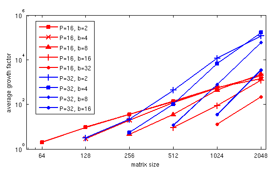
Figure 8: Growth factor of block parallel LU_PRRP for varying block size $b$ and number of processors $P$.

The upper bound of the growth factor of both block parallel and block pairwise LU_PRRP is $(1+\tau b)^{n\over b}$, since for every panel factorization, a row is updated only once. Hence they have the same bounds as the LU_PRRP factorization, and smaller than that of the CALU_PRRP factorization. Despite this, they are less stable than the CALU_PRRP factorization. Figures 8 and 9 display the growth factor of block parallel LU_PRRP and block pairwise LU_PRRP for matrices following a normal distribution. In figure 8, the number of processors $P$ on which each panel is partitioned is varying from 16 to 32, and the block size $b$ is varying from $2$ to $16$. The matrix size varies from $64$ to $2048$, but we have observed the same behavior for matrices of size up to $8192$. When the number of processors $P$ is equal to $1$, the block parallel LU_PRRP corresponds to the LU_PRRP factorization. The results show that there are values of $P$ and $b$ for which this method can be very unstable. For the sizes of matrices tested, when $b$ is chosen such that the blocks at the leaves of the reduction tree have more than $2b$ rows, the number of processors $P$ has an important impact, the growth factor increases with increasing $P$, and the method is unstable.

In Figure 9, the matrix size varies from $1024$ to $8192$. For a given matrix size, the growth factor increases with decreasing the size of the panel $b$, as one could expect. We note that the growth factor of block pairwise LU_PRRP is larger than that obtained with the CALU_PRRP factorization based on a flat tree scheme presented in Table 21. But it stays smaller than the size of the matrix $n$ for different panel sizes. Hence this method is more stable than block parallel LU_PRRP. Further investigation is required to conclude on the stability of these methods.

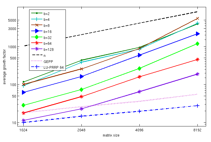
Figure 9: Growth factor of block pairwise LU_PRRP for varying matrix size and varying block size $b$.

6 Conclusions

This paper introduces LU_PRRP, an LU factorization algorithm based on panel rank revealing pivoting. This algorithm is more stable than GEPP in terms of worst case growth factor. It is also very stable in practice for various classes of matrices, including pathological cases on which GEPP fails.

Its communication avoiding version, CALU_PRRP, is also more stable in terms of worst case growth factor than CALU, the communication avoiding version of GEPP. More importantly, there are cases of interest for which the upper bound of the growth factor of CALU_PRRP is smaller than that of GEPP for several cases of interest. Extensive experiments show that CALU_PRRP is very stable in practice and leads to results of the same order of magnitude as GEPP, sometimes even better.

Our future work focuses on two main directions. The first direction investigates the design of a communication avoiding algorithm that has smaller bounds on the growth factor than that of GEPP in general. The second direction focuses on estimating the performance of CALU_PRRP on parallel machines based on multicore processors, and comparing it with the performance of CALU.

Appendix A

We describe briefly strong RRQR introduced by M. Gu and S. Eisenstat in [12]. This factorization will be used in our new LU decomposition algorithm, which aims to obtain an upper bound of the growth factor smaller than GEPP (see Section 2.) Consider a given threshold $\tau>1$ and an $h\times p$ matrix $B$ with $p>h$, a Strong RRQR factorization on a matrix $B$ gives (with an empty $(2,2)$ block)

$$B^{T}\Pi=QR=Q\left[\begin{array}[]{cc}R_{11}&R_{12}\\ \end{array}\right],$$

where $\lVert R_{11}^{-1}R_{12}\rVert_{max}\leq\tau$, with $\lVert\ .\ \rVert_{max}$ being the biggest entry of a given matrix in absolute value. This factorization can be computed by a classical QR factorization with column pivoting followed by a limited number of additional swaps and QR updates if necessary.

Algorithm 2 Strong RRQR

1:Compute $B^{T}\Pi=QR$ using the classical RRQR with column pivoting

2:while there exist i and j such that $\lvert{(R_{11}^{-1}R_{12})}_{ij}\rvert>\tau$  do

3:     Set $\Pi=\Pi\Pi_{ij}$ and compute the QR factorization of $R$ $\Pi_{ij}$ (QR updates)

4:end while

5:$B^{T}\Pi=QR$ with $\lVert R_{11}^{-1}R_{12}\rVert_{max}\leq\tau$

The while loop in Algorithm 2 interchanges any pairs of columns that can increase $\lvert det(R_{11})\rvert$ by at least a factor $\tau$. At most $O(\log_{\tau}n)$ such interchanges are necessary before Algorithm 2 finds a strong RRQR factorization. The QR factorization of $B^{T}\Pi$ can be computed numerically via efficient and numerically stable QR updating procedures. See [12] for details.

Appendix B

We present experimental results for the LU_PRRP factorization, the binary tree based CALU_PRRP, and the flat tree based CALU_PRRP. We show results obtained for the LU decomposition and the linear solver. Tables 16, 21, and 23 display the results obtained for random matrices. They show the growth factor, the norm of the factor L and U and their inverses, and the relative error of the decomposition.
Tables 17, 18, 22, and 24 display the results obtained for the special matrices presented in Table LABEL:Tab_allTestMatrix. The size of the tested matrices is n = 4096. For LU_PRRP and flat tree based CALU_PRRP, the size of the panel is $b=8$. For binary tree based CALU_PRRP we use $P=64$ and $b=8$, this means that the size of the matrices used at the leaves of the reduction tree is $64\times 8$.
Tables 19 and 20 present results for the linear solver using binary tree based and flat tree based CALU_PRRP, together with CALU and GEPP for comparison.
The tables are presented in the following order.

• Table 16: Stability of the LU decomposition for LU_PRRP and GEPP on random matrices.

• Table 17: Stability of the LU decomposition for GEPP on special matrices.

• Table 18: Stability of the LU decomposition for LU_PRRP on special matrices.

• Table 19: Stability of the linear solver using binary tree based CALU_PRRP, binary tree based CALU, and GEPP.

• Table 20: Stability of the linear solver using flat tree based CALU_PRRP, flat tree based CALU, and GEPP.

• Table 21: Stability of the LU decomposition for flat tree based CALU_PRRP and GEPP on random matrices.

• Table 22: Stability of the LU decomposition for flat tree based CALU_PRRP on special matrices.

• Table 23: Stability of the LU decomposition for binary tree based CALU_PRRP and GEPP on random matrices.

• Table 24: Stability of the LU decomposition for binary tree based CALU_PRRP on special matrices.

Table 15: Special matrices in our test set.

No.	Matrix	Remarks
1	hadamard	Hadamard matrix, hadamard($n$), where $n$, $n/12$, or $n/20$ is power of 2.
2	house	Householder matrix, $A=\mathrm{eye}(n)-\beta*v*v^{\prime}$, where $[v,\beta,s]$ = gallery(’house’, randn($n$, 1)).
3	parter	Parter matrix, a Toeplitz matrix with most of singular values near $\pi$. gallery(’parter’, $n$), or $A(i,j)=1/(i-j+0.5)$.
4	ris	Ris matrix, matrix with elements $A(i,j)=0.5/(n-i-j+1.5)$. The eigenvalues cluster around $-\pi/2$ and $\pi/2$. gallery(’ris’, $n$).
5	kms	Kac-Murdock-Szego Toeplitz matrix. Its inverse is tridiagonal. gallery(’kms’, $n$) or gallery(’kms’, $n$, rand).
6	toeppen	Pentadiagonal Toeplitz matrix (sparse).
7	condex	Counter-example matrix to condition estimators. gallery(’condex’, $n$).
8	moler	Moler matrix, a symmetric positive definite (spd) matrix. gallery(’moler’, $n$).
9	circul	Circulant matrix, gallery(’circul’, randn($n$, 1)).
10	randcorr	Random $n\times n$ correlation matrix with random eigenvalues from a uniform distribution, a symmetric positive semi-definite matrix. gallery(’randcorr’, $n$).
11	poisson	Block tridiagonal matrix from Poisson’s equation (sparse), $A$ = gallery(’poisson’,sqrt($n$)).
12	hankel	Hankel matrix, $A$ = hankel($c,r$), where $c$=randn($n$, 1), $r$=randn($n$, 1), and $c(n)=r(1)$.
13	jordbloc	Jordan block matrix (sparse).
14	compan	Companion matrix (sparse), $A$ = compan(randn($n$+1,1)).
15	pei	Pei matrix, a symmetric matrix. gallery(’pei’, $n$) or gallery(’pei’, $n$, randn).
16	randcolu	Random matrix with normalized cols and specified singular values. gallery(’randcolu’, $n$).
17	sprandn	Sparse normally distributed random matrix, $A$ = sprandn($n,n$,0.02).
18	riemann	Matrix associated with the Riemann hypothesis. gallery(’riemann’, $n$).
19	compar	Comparison matrix, gallery(’compar’, randn($n$), unidrnd(2)$-1$).
20	tridiag	Tridiagonal matrix (sparse).
21	chebspec	Chebyshev spectral differentiation matrix, gallery(’chebspec’, $n$, 1).
22	lehmer	Lehmer matrix, a symmetric positive definite matrix such that $A(i,j)=i/j$ for $j\geq i$. Its inverse is tridiagonal. gallery(’lehmer’, $n$).
23	toeppd	Symmetric positive semi-definite Toeplitz matrix. gallery(’toeppd’, $n$).
24	minij	Symmetric positive definite matrix with $A(i,j)=\min(i,j)$. gallery(’minij’, $n$).
25	randsvd	Random matrix with preassigned singular values and specified bandwidth. gallery(’randsvd’, $n$).
26	forsythe	Forsythe matrix, a perturbed Jordan block matrix (sparse).
27	fiedler	Fiedler matrix, gallery(’fiedler’, $n$), or gallery(’fiedler’, randn($n$, 1)).
28	dorr	Dorr matrix, a diagonally dominant, ill-conditioned, tridiagonal matrix (sparse).
29	demmel	$A=D*$(eye$(n)+10^{-7}*$rand($n$)), where $D=$ diag($10^{14*(0:n-1)/n}$) [3].
30	chebvand	Chebyshev Vandermonde matrix based on $n$ equally spaced points on the interval $[0,1]$. gallery(’chebvand’, $n$).
31	invhess	$A$=gallery(’invhess’, $n$, rand($n-1,1$)). Its inverse is an upper Hessenberg matrix.
32	prolate	Prolate matrix, a spd ill-conditioned Toeplitz matrix. gallery(’prolate’, $n$).
33	frank	Frank matrix, an upper Hessenberg matrix with ill-conditioned eigenvalues.
34	cauchy	Cauchy matrix, gallery(’cauchy’, randn($n$, 1), randn($n$, 1)).
35	hilb	Hilbert matrix with elements $1/(i+j-1)$. $A=$hilb($n$).
36	lotkin	Lotkin matrix, the Hilbert matrix with its first row altered to all ones. gallery(’lotkin’, $n$).
37	kahan	Kahan matrix, an upper trapezoidal matrix.

Table 16: Stability of the LU decomposition for LU_PRRP and GEPP on random matrices.

LU_PRRP
n	b	$g_{W}$	$||U||_{1}$	$||U^{-1}||_{1}$	$\frac{||PA-LU||_{F}}{||A||_{F}}$	HPL1	HPL2	HPL3
8192	128	2.38E+01	9.94E+04	3.34E+02	5.26E-14	4.13E-02	2.35E-02	4.68E-03
	64	2.76E+01	1.07E+05	1.06E+03	5.24E-14	5.38E-02	2.08E-02	4.36E-03
	32	3.15E+01	1.20E+05	3.38E+02	5.14E-14	3.95E-02	2.27E-02	4.54E-03
	16	3.63E+01	1.32E+05	3.20E+02	4.91E-14	3.29E-02	1.89E-02	3.79E-03
	8	3.94E+01	1.41E+05	2.65E+02	4.84E-14	2.95E-02	1.69E-02	3.37E-03
4096	128	1.75E+01	3.74E+04	4.34E+02	2.69E-14	3.28E-02	2.21E-02	4.58E-03
	64	1.96E+01	4.09E+04	1.02E+03	2.62E-14	2.10E-01	2.17E-02	4.64E-03
	32	2.33E+01	4.51E+04	2.22E+03	2.56E-14	5.78E-2	2.10E-02	4.51E-03
	16	2.61E+01	4.89E+04	1.15E+03	2.57E-14	2.98E-01	1.99E-02	4.08E-03
	8	2.91E+01	5.36E+04	1.93E+03	2.60E-14	2.36E-01	1.82E-02	3.90E-03
2048	128	1.26E+01	1.39E+04	5.61E+02	1.46E-14	4.37E-02	2.25E-02	5.16E-03
	64	1.46E+01	1.52E+04	1.86E+02	1.42E-14	4.25E-02	2.24E-02	5.05E-03
	32	1.56E+01	1.67E+04	3.48E+03	1.38E-14	7.53E-1	2.15E-02	4.65E-03
	16	1.75E+01	1.80E+04	2.59E+02	1.38E-14	2.51E-02	2.03E-02	4.59E-03
	8	2.06E+01	2.00E+04	5.00E+02	1.40E-14	4.46E-02	1.93E-02	4.33E-03
1024	128	8.04E+00	5.19E+03	5.28E+02	7.71E-15	9.92E-02	2.26E-02	5.45E-03
	64	9.93E+00	5.68E+03	5.28E+02	7.73E-15	4.36E-02	2.13E-02	4.88E-03
	32	1.13E+01	6.29E+03	3.75E+02	7.51E-15	7.90E-02	2.09E-02	4.74E-03
	16	1.31E+01	6.91E+03	1.51E+02	7.55E-15	2.10E-02	1.93E-02	4.08E-03
	8	1.44E+01	7.54E+03	4.16E+03	7.55E-15	1.34E+00	1.84E-02	4.25E-03
GEPP
8192	-	5.47E+01	8.71E+03	6.03E+02	7.23E-14	1.34E-02	1.36E-02	2.84E-03
4096	-	3.61E+01	1.01E+03	1.87E+02	3.88E-14	1.83E-02	1.43E-02	2.90E-03
2048	-	2.63E+01	5.46E+02	1.81E+02	2.05E-14	2.88E-02	1.54E-02	3.37E-03
1024	-	1.81E+01	2.81E+02	4.31E+02	1.06E-14	5.78E-02	1.62E-02	3.74E-03

Table 17: Stability of the LU decomposition for GEPP on special matrices.

matrix

cond(A,2)

$g_{W}$

$||L||_{1}$

$||L^{-1}||_{1}$

${\max\atop{ij}}|U_{ij}|$

${\min\atop{kk}}|U_{kk}|$

cond($U$,1)

$\frac{||PA-LU||_{F}}{||A||_{F}}$

$\eta$

$w_{b}$

$N_{IR}$

well-conditioned

hadamard

1.0E+0

4.1E+3

4.1E+3

4.1E+3

4.1E+3

1.0E+0

5.3E+5

0.0E+0

3.3E-16

4.6E-15

2

house

1.0E+0

5.1E+0

8.9E+2

2.6E+2

5.1E+0

5.7

1.4E+4

2.0E-15

5.6E-17

6.3E-15

3

parter

4.8E+0

1.6E+0

4.8E+1

2.0E+0

3.1E+0

2.0E+0

2.3E+2

2.3E-15

8.3E-16

4.4E-15

3

ris

4.8E+0

1.6E+0

4.8E+1

2.0E+0

1.6E+0

1.0E+0

2.3E+2

2.3E-15

7.1E-16

4.7E-15

2

kms

9.1E+0

1.0E+0

2.0E+0

1.5E+0

1.0E+0

7.5E-1

3.0E+0

2.0E-16

1.1E-16

6.7E-16

1

toeppen

1.0E+1

1.1E+0

2.1E+0

9.0E+0

1.1E+1

1.0E+1

3.3E+1

1.1E-17

7.2E-17

3.0E-15

1

condex

1.0E+2

1.0E+0

2.0E+0

5.6E+0

1.0E+2

1.0E+0

7.8E+2

1.8E-15

9.7E-16

6.8E-15

3

moler

1.9E+2

1.0E+0

2.2E+1

2.0E+0

1.0E+0

1.0E+0

4.4E+1

3.8E-14

2.6E-16

1.7E-15

2

circul

3.7E+2

1.8E+2

1.0E+3

1.4E+3

6.4E+2

3.4E+0

1.2E+6

4.3E-14

2.1E-15

1.2E-14

1

randcorr

1.4E+3

1.0E+0

3.1E+1

5.7E+1

1.0E+0

2.3E-1

5.0E+4

1.6E-15

7.8E-17

8.0E-16

1

poisson

1.7E+3

1.0E+0

2.0E+0

3.4E+1

4.0E+0

3.2E+0

7.8E+1

2.8E-16

1.4E-16

7.5E-16

1

hankel

2.9E+3

6.2E+1

9.8E+2

1.5E+3

2.4E+2

4.5E+0

2.0E+6

4.2E-14

2.5E-15

1.6E-14

2

jordbloc

5.2E+3

1.0E+0

1.0E+0

1.0E+0

1.0E+0

1.0E+0

8.2E+3

0.0E+0

2.0E-17

8.3E-17

0

compan

7.5E+3

1.0E+0

2.0E+0

4.0E+0

7.9E+0

2.6E-1

7.8E+1

0.0E+0

2.0E-17

6.2E-13

1

pei

1.0E+4

1.0E+0

4.1E+3

9.8E+0

1.0E+0

3.9E-1

2.5E+1

7.0E-16

6.6E-18

2.3E-17

0

randcolu

1.5E+4

4.6E+1

9.9E+2

1.4E+3

3.2E+0

5.6E-02

1.1E+7

4.0E-14

2.3E-15

1.4E-14

1

sprandn

1.6E+4

7.4E+0

7.4E+2

1.5E+3

2.9E+1

1.7E+0

1.3E+7

3.4E-14

8.5E-15

9.3E-14

2

riemann

1.9E+4

1.0E+0

4.1E+3

3.5E+0

4.1E+3

1.0E+0

2.6E+6

5.7E-19

2.0E-16

1.7E-15

2

compar

1.8E+6

2.3E+1

9.8E+2

1.4E+3

1.1E+2

3.1E+0

2.7E+7

2.3E-14

1.2E-15

8.8E-15

1

tridiag

6.8E+6

1.0E+0

2.0E+0

1.5E+3

2.0E+0

1.0E+0

5.1E+3

1.4E-18

2.6E-17

1.2E-16

0

chebspec

1.3E+7

1.0E+0

5.4E+1

9.2E+0

7.1E+6

1.5E+3

4.2E+7

1.8E-15

2.9E-18

1.6E-15

1

lehmer

1.8E+7

1.0E+0

1.5E+3

2.0E+0

1.0E+0

4.9E-4

8.2E+3

1.5E-15

2.8E-17

1.7E-16

0

toeppd

2.1E+7

1.0E+0

4.2E+1

9.8E+2

2.0E+3

2.9E+2

1.3E+6

1.5E-15

5.0E-17

3.3E-16

1

minij

2.7E+7

1.0E+0

4.1E+3

2.0E+0

1.0E+0

1.0E+0

8.2E+3

0.0E+0

7.8E-19

4.2E-18

0

randsvd

6.7E+7

4.7E+0

9.9E+2

1.4E+3

6.4E-02

3.6E-7

1.4E+10

5.6E-15

3.4E-16

2.0E-15

2

forsythe

6.7E+7

1.0E+0

1.0E+0

1.0E+0

1.0E+0

1.5E-8

6.7E+7

0.0E+0

0.0E+0

0.0E+0

0

ill-conditioned

fiedler

2.5E+10

1.0E+0

1.7E+3

1.5E+1

7.9E+0

4.1E-7

2.9E+8

1.6E-16

3.3E-17

1.0E-15

1

dorr

7.4E+10

1.0E+0

2.0E+0

3.1E+2

3.4E+5

1.3E+0

1.7E+11

6.0E-18

2.3E-17

2.2E-15

1

demmel

1.0E+14

2.5E+0

1.2E+2

1.4E+2

1.6E+14

7.8E+3

1.7E+17

3.7E-15

7.1E-21

4.8E-9

2

chebvand

3.8E+19

2.0E+2

2.2E+3

3.1E+3

1.8E+2

9.0E-10

4.8E+22

5.1E-14

3.3E-17

2.6E-16

1

invhess

4.1E+19

2.0E+0

4.1E+3

2.0E+0

5.4E+0

4.9E-4

3.0E+48

1.2E-14

1.7E-17

2.4E-14

(1)

prolate

1.4E+20

1.2E+1

1.4E+3

4.6E+3

5.3E+0

5.9E-13

4.7E+23

1.6E-14

4.7E-16

6.3E-15

(1)

frank

1.7E+20

1.0E+0

2.0E+0

2.0E+0

4.1E+3

5.9E-24

1.9E+30

2.2E-18

4.9E-27

1.2E-23

0

cauchy

5.5E+21

1.0E+0

3.1E+2

1.9E+2

1.0E+7

2.3E-15

2.1E+24

1.4E-15

6.1E-19

5.2E-15

(1)

hilb

8.0E+21

1.0E+0

3.1E+3

1.3E+3

1.0E+0

4.2E-20

2.2E+22

2.2E-16

6.0E-19

2.0E-17

0

lotkin

5.4E+22

1.0E+0

2.6E+3

1.3E+3

1.0E+0

3.6E-19

2.3E+22

8.0E-17

3.0E-18

2.3E-15

(1)

kahan

1.1E+28

1.0E+0

1.0E+0

1.0E+0

1.0E+0

2.2E-13

4.1E+53

0.0E+0

9.7E-18

4.3E-16

1

Table 18: Stability of the LU decomposition for LU_PRRP on special matrices.

	matrix	cond(A,2)	$g_{W}$	$||L||_{1}$	$||L^{-1}||_{1}$	$||U||_{1}$	$||U^{-1}||_{1}$	$\frac{||PA-LU||_{F}}{||A||_{F}}$	$\eta$	$w_{b}$	$N_{IR}$
well-conditioned	hadamard	1.0E+0	5.1E+02	5.1E+02	2.5E+16	5.6E+0	6.0E+00	5.2E-15	1.1E-15	9.0E-15	2
	house	1.0E+0	7.4E+00	8.3E+02	7.9E+02	3.7E+02	5.0E+01	5.8E-16	4.2E-17	4.8E-15	(2)
	parter	4.8E+0	1.5E+00	4.7E+01	3.7E+00	1.4E+01	3.6E+01	8.5E-16	6.8E-16	4.4E-15	3
	ris	4.8E+0	1.5E+00	4.7E+01	1.1E+01	7.3E+00	7.2E+01	8.5E-16	7.6E-16	4.6E-15	2
	kms	9.1E+0	1.0E+00	6.7E+00	4.0E+00	4.1E+00	1.2E+01	1.4E-16	6.8E-17	3.7E-16	1
	toeppen	1.0E+1	1.3E+00	2.3E+00	3.4E+00	3.6E+01	1.0E+00	1.3E-16	8.3E-17	2.2E-15	1
	condex	1.0E+2	1.0E+00	1.9E+00	5.5E+00	5.9E+02	1.2E+00	6.5E-16	7.4E-16	5.1E-15	(2)
	moler	1.9E+2	1.0E+00	2.7E+03	3.9E+02	1.3E+05	3.0E+15	8.1E-16	3.9E-19	3.4E-17	0
	circul	3.7E+2	1.4E+02	1.0E+03	6.7E+17	7.4E+04	1.3E+01	3.7E-14	3.2E-15	2.1E-14	2
	randcorr	1.4E+3	1.0E+00	3.0E+01	3.7E+01	3.5E+01	2.4E+04	5.8E-16	5.9E-17	5.5E-16	1
	poisson	1.7E+3	1.0E+00	1.9E+00	2.0E+01	7.32E+00	2.0E+01	1.6E-16	9.1E-17	1.8E-15	1
	hankel	2.9E+3	5.0E+01	1.0E+03	1.8E+17	5.7E+04	3.3E+01	3.5E-14	2.8E-15	1.7E-14	2
	jordbloc	5.2E+3	1.0E+00	1.0E+00	1.0E+00	2.0E+00	4.0E+03	0.0E+00	1.9E-17	6.1E-17	0
	compan	7.5E+3	1.0E+00	2.9E+00	3.9E+01	6.8E+02	4.1E+00	6.7E-16	5.5E-16	6.9E-12	1
	pei	1.0E+4	4.9E+00	2.8E+03	1.6E+01	1.7E+01	1.7E+01	6.5E-16	1.4E-17	3.2E-17	0
	randcolu	1.5E+4	3.3E+01	1.1E+03	1.5E+17	8.8E+02	1.3E+04	3.5E-14	2.9E-15	1.8E-14	2
	sprandn	1.6E+4	4.9E+00	7.8E+02	1.4E+17	8.8E+03	5.4E+03	3.1E-14	1.0E-14	1.3E-13	2
	riemann	1.9E+4	1.0E+00	4.0E+03	1.0E+03	3.1E+06	1.4E+02	4.5E-16	1.5E-16	2.0E-15	1
	compar	1.8E+6	9.0E+02	1.7E+03	9.8E+16	9.0E+05	8.0E+02	1.4E-14	1.1E-15	7.7E-15	1
	tridiag	6.8E+6	1.0E+00	1.9E+00	2.0E+02	4.0E+00	1.6E+04	3.2E-16	2.8E-17	2.4E-16	0
	chebspec	1.3E+7	1.0E+00	5.2E+01	1.6E+24	9.7E+06	1.7E+00	5.9E-16	1.0E-18	5.0E-15	1
	lehmer	1.8E+7	1.0E+00	1.5E+03	9.5E+00	8.90E+00	8.1E+03	5.6E-16	1.00E-17	6.1E-17	0
	toeppd	2.1E+7	1.0E+00	4.2E+01	1.2E+02	6.69E+04	7.2E+01	5.8E-16	2.6E-17	1.6E-16	0
	minij	2.7E+7	1.0E+00	4.0E+03	1.1E+03	1.7E+06	4.0E+00	5.3E-16	1.1E-18	1.3E-16	0
	randsvd	6.7E+7	3.9E+00	1.1E+03	3.2E+17	5.4E+00	2.5E+09	5.0E-15	4.6E-16	2.9E-15	2
	forsythe	6.7E+7	1.0E+00	1.0E+00	1.0E+00	1.0E+00	6.7E+07	0.0E+00	0.0E+00	0.0E+00	0
ill-conditioned	fiedler	2.5E+10	1.0E+00	9.3E+02	3.06E+03	6.5E+01	1.5E+07	2.4E-16	9.9E-17	2.0E-15	1
	dorr	7.4E+10	1.0E+00	2.0E+00	5.4E+01	6.7E+05	2.5E+05	1.6E-16	3.4E-17	4.0E-15	1
	demmel	1.0E+14	1.3E+00	1.1E+02	1.7E+16	5.0E+15	2.5E+01	3.2E-15	9.1E-21	1.1E-08	2
	chebvand	3.8E+19	1.8E+02	1.4E+03	1.2E+17	7.3E+04	4.3E+19	5.3E-14	4.0E-17	2.3E-16	0
	invhess	4.1E+19	2.1E+00	4.0E+03	7.4E+03	5.8E+03	1.0E+22	1.4E-15	2.5E-17	3.3E-14	1
	prolate	1.4E+20	8.9E+00	1.3E+03	1.4E+18	1.4E+03	9.7E+20	1.9E-14	1.0E-15	2.6E-14	1
	frank	1.7E+20	1.0E+00	1.9E+00	1.9E+00	4.1E+06	2.3E+16	1.6E-17	1.8E-20	6.2E-17	0
	cauchy	5.5E+21	1.0E+00	3.3E+02	2.0E+06	6.9E+07	1.8E+20	6.0E-16	3.9E-19	1.5E-14	1
	hilb	8.0E+21	1.0E+00	3.0E+03	1.1E+18	2.4E+00	3.1E+22	3.2E-16	6.6E-19	2.3E-17	0
	lotkin	5.4E+22	1.0E+00	2.6E+03	2.0E+18	2.4E+00	8.1E+22	6.6E-17	2.3E-18	1.0E-15	0
	kahan	1.1E+28	1.0E+00	1.0E+00	1.0E+00	5.3E+00	7.6E+52	0E+00	1.1E-17	5.2E-16	1

Table 19: Stability of the linear solver using binary tree based CALU_PRRP, binary tree based CALU, and GEPP.

n	P	b	$\eta$	$w_{b}$	$N_{IR}$	HPL1	HPL2	HPL3
Binary tree based CALU_PRRP
8192	256	32	7.5E-15	4.4E-14	2	6.2E-02	2.3E-02	4.4E-03
		16	6.7E-15	4.1E-14	2	3.4E-02	2.2E-02	4.6E-03
	128	64	7.6E-15	4.7E-14	2	2.6E-02	2.5E-02	4.9E-03
		32	7.5E-15	4.9E-14	2	6.9E-02	2.6E-02	4.9E-03
		16	7.3E-15	5.1E-14	2	4.2E-02	2.7E-02	5.7E-03
	64	128	7.6E-15	5.0E-14	2	2.8E-02	2.6E-02	5.2E-03
		64	7.9E-15	5.3E-14	2	6.2E-02	2.8E-02	5.9E-03
		32	7.8E-15	5.0E-14	2	7.0E-02	2.6E-02	5.0E-03
		16	6.7E-15	5.0E-14	2	4.2E-02	2.7E-02	5.7E-03
4096	256	16	3.5E-15	2.2E-14	2	5.8E-02	2.3E-02	5.1E-03
	128	32	3.8E-15	2.3E-14	2	5.3E-02	2.4E-02	5.1E-03
		16	3.6E-15	2.2E-14	1.6	1.3E-02	2.4E-02	5.1E-03
	64	64	4.0E-15	2.3E-14	2	3.8E-02	2.4E-02	4.9E-03
		32	3.9E-15	2.4E-14	2	1.2 E-02	2.5E-02	5.7E-03
		16	3.8E-15	2.4E-14	1.6	2.3E-02	2.5E-02	5.2E-03
2048	128	16	1.8E-15	1.0E-14	2	8.1E-02	2.2E-02	4.8E-03
	64	32	1.8E-15	1.2E-14	2	9.7E-02	2.5E-02	5.6E-03
		16	1.9E-15	1.2E-14	1.8	3.4E-02	2.5E-02	5.4E-03
1024	64	16	1.0E-15	6.3E-15	1.3	7.2E-02	2.5E-02	6.1E-03
Binary tree based CALU
8192	256	32	6.2E-15	4.1E-14	2	3.6E-02	2.2E-02	4.5E-03
		16	5.8E-15	3.9E-14	2	4.5E-02	2.1E-02	4.1E-03
	128	64	6.1E-15	4.2E-14	2	5.0E-02	2.2E-02	4.6E-03
		32	6.3E-15	4.0E-14	2	2.5E-02	2.1E-02	4.4E-03
		16	5.8E-15	4.0E-14	2	3.8E-02	2.1E-02	4.3E-03
	64	128	5.8E-15	3.6E-14	2	8.3E-02	1.9E-02	3.9E-03
		64	6.2E-15	4.3E-14	2	3.2E-02	2.3E-02	4.4E-03
		32	6.3E-15	4.1E-14	2	4.4E-02	2.2E-02	4.5E-03
		16	6.0E-15	4.1E-14	2	3.4E-02	2.2E-02	4.2E-03
4096	256	16	3.1E-15	2.1E-14	1.7	3.0E-02	2.2E-02	4.4E-03
	128	32	3.2E-15	2.3E-14	2	3.7E-02	2.4E-02	5.1E-03
		16	3.1E-15	1.8E-14	2	5.8E-02	1.9E-02	4.0E-03
	64	64	3.2E-15	2.1E-14	1.7	3.1E-02	2.2E-02	4.6E-03
		32	3.2E-15	2.2E-14	1.3	3.6E-02	2.3E-02	4.7E-03
		16	3.1E-15	2.0E-14	2	9.4E-02	2.1E-02	4.3E-03
2048	128	16	1.7E-15	1.1E-14	1.8	6.9E-02	2.3E-02	5.1E-03
	64	32	1.7E-15	1.0E-14	1.6	6.5E-02	2.1E-02	4.6E-03
		16	1.6E-15	1.1E-14	1.8	4.7E-02	2.2E-02	4.9E-03
1024	64	16	8.7E-16	5.2E-15	1.6	1.2E-1	2.1E-02	4.7E-03
GEPP
8192	-		3.9E-15	2.6E-14	1.6	1.3E-02	1.4E-02	2.8E-03
4096	-		2.1E-15	1.4E-14	1.6	1.8E-02	1.4E-02	2.9E-03
2048	-		1.1E-15	7.4E-15	2	2.9E-02	1.5E-02	3.4E-03
1024	-		6.6E-16	4.0E-15	2	5.8E-02	1.6E-02	3.7E-03

Table 20: Stability of the linear solver using flat tree based CALU_PRRP, flat tree based CALU, and GEPP.

n	P	b	$\eta$	$w_{b}$	$N_{IR}$	HPL1	HPL2	HPL3
Flat tree based CALU_PRRP
8096	-	8	6.2E-15	3.8E-14	1	1.7E-02	2.0E-02	4.0E-03
	-	16	6.6E-15	4.3E-14	1	3.6E-02	2.2E-02	4.3E-03
	-	32	7.2E-15	4.8E-14	1	6.5E-02	2.5E-02	5.3E-03
	-	64	7.3E-15	5.1E-14	1	4.8E-02	2.7E-02	5.4E-03
4096	-	8	3.2E-15	2.0E-14	1	6.7E-02	2.1E-02	4.7E-03
	-	16	3.6E-15	2.3E-14	1	2.9E-02	2.4E-02	5.1E-03
	-	32	3.8E-15	2.4E-14	1	4.6E-02	2.5E-02	5.5E-03
	-	64	3.7E-15	2.5E-14	1	1.7E-1	2.6E-02	5.6E-03
2048	-	8	1.4E-15	1.1E-14	1	1.3E-1	2.3E-02	5.1E-03
	-	16	1.9E-15	1.1E-14	1	1.6E+0	2.3 E-02	5.3E-03
	-	32	2.1E-15	1.3E-14	1	2.5E-02	2.7E-02	5.8E-03
	-	64	1.9E-15	1.25E-14	1	1.2E-1	2.6E-02	5.9E-03
1024	-	8	9.4E-16	5.5E-15	1	3.8E-02	2.2E-02	5.3E-03
	-	16	1.0E-15	6.0E-15	1	6.2E-02	2.4E-02	5.4E-03
	-	32	1.0E-15	5.6E-15	1	4.2E-02	2.2E-02	5.4E-03
	-	64	1.0E-15	6.8E-15	1	3.6E-02	2.7E-02	6.7E-03
Flat tree based CALU
8096	-	8	4.5E-15	3.1E-14	1.7	4.4E-02	1.6E-02	3.4E-03
	-	16	5.6E-15	3.7E-14	2	1.9E-02	2.0E-02	3.3E-03
	-	32	6.7E-15	4.4E-14	2	4.6E-02	2.4E-02	4.7E-03
	-	64	6.5E-15	4.2E-14	2	5.5E-02	2.2E-02	4.6E-03
4096	-	8	2.6E-15	1.7E-14	1.3	1.3E-02	1.8E-02	4.0E-03
	-	16	3.0E-15	1.9E-14	1.7	2.6E-02	2.0E-02	3.9E-03
	-	32	3.8E-15	2.4E-14	2	1.9E-02	2.5E-02	5.1E-03
	-	64	3.4E-15	2.0E-14	2	6.0E-02	2.1E-02	4.1E-03
2048	-	8	1.5E-15	8.7E-15	1.6	2.7E-02	1.8E-02	4.2E-03
	-	16	1.6E-15	1.0E-14	2	2.1E-1	2.1E-02	4.5E-03
	-	32	1.8E-15	1.1E-14	1.8	2.3E-1	2.3E-02	5.1E-03
	-	64	1.7E-15	1.0E-14	1.2	4.1E-02	2.1E-02	4.5E-03
1024	-	8	7.8E-16	4.9E-15	1.6	5.5E-02	2.0E-02	4.9E-03
	-	16	9.2E-16	5.2E-15	1.2	1.1E-1	2.1E-02	4.8E-03
	-	32	9.6E-16	5.8E-15	1.1	1.5E-1	2.3E-02	5.6E-03
	-	64	8.7E-16	4.9E-15	1.3	7.9E-02	2.0E-02	4.5E-03
GEPP
8192	-		3.9E-15	2.6E-14	1.6	1.3E-02	1.4E-02	2.8E-03
4096	-		2.1E-15	1.4E-14	1.6	1.8E-02	1.4E-02	2.9E-03
2048	-		1.1E-15	7.4E-15	2	2.9E-02	1.5E-02	3.4E-03
1024	-		6.6E-16	4.0E-15	2	5.8E-02	1.6E-02	3.7E-03

Table 21: Stability of the LU decomposition for flat tree based CALU_PRRP and GEPP on random matrices

Flat Tree based CALU_PRRP
n	b	$g_{W}$	$||L||_{1}$	$||L^{-1}||_{1}$	$||U||_{1}$	$||U^{-1}||_{1}$	$\frac{||PA-LU||_{F}}{||A||_{F}}$	HPL1	HPL2	HPL3
8192	128	3.44E+01	2.96E+03	2.03E+03	1.29E+05	2.86E+03	8.67E-14	1.77E-01	2.53E-02	5.00E-03
	64	4.42E+01	3.30E+03	2.28E+03	1.43E+05	6.89E+02	8.56E-14	3.62E-02	2.97E-02	6.40E-03
	32	5.88E+01	4.34E+03	2.50E+03	1.54E+05	3.79E+02	8.15E-14	3.40E-02	2.96E-02	6.40E-03
	16	6.05E+01	4.54E+03	2.50E+03	1.53E+05	4.57E+02	6.59E-14	5.66E-02	2.27E-02	4.60E-03
	8	5.25E+01	3.24E+03	2.63E+03	1.60E+05	1.78E+02	5.75E-14	1.92E-02	1.93E-02	4.10E-03
4096	128	2.38E+01	1.60E+03	1.05E+03	4.75E+04	5.11E+03	4.15E-14	1.58E+00	2.40E-02	5.16E-03
	64	2.90E+01	1.85E+03	1.19E+03	5.18E+04	2.38E+03	4.55E-14	1.71E-01	2.60E-02	5.65E-03
	32	3.32E+01	1.89E+03	1.29E+03	5.57E+04	3.04E+02	4.63E-14	4.63E-02	2.57E-02	5.51E-03
	16	3.87E+01	1.94E+03	1.34E+03	5.90E+04	2.62E+02	4.54E-14	2.92E-02	2.44E-02	5.18E-03
	8	3.80E+01	1.63E+03	1.36E+03	5.90E+04	5.63E+02	4.24E-14	6.70E-02	2.19E-02	4.73E-03
2048	128	1.57E+01	6.90E+02	5.26E+02	1.66E+04	3.79E+02	2.01E-14	6.29E-02	2.43E-02	5.39E-03
	64	1.80E+01	7.94E+02	6.06E+02	1.86E+04	4.22E+02	2.25E-14	1.26E-01	2.63E-02	5.96E-03
	32	2.19E+01	9.30E+02	6.86E+02	2.05E+04	1.08E+02	2.41E-14	2.59E-02	2.70E-02	5.80E-03
	16	2.53E+01	8.62E+02	6.99E+02	2.17E+04	3.50E+02	2.36E-14	1.68E+00	2.30E-02	5.36E-03
	8	2.62E+01	8.32E+02	7.19E+02	2.21E+04	4.58E+02	2.27E-14	1.37E-01	2.36E-02	5.13E-03
1024	128	9.36E+00	3.22E+02	2.59E+02	5.79E+03	9.91E+02	9.42E-15	3.98E-02	2.50E-02	5.77E-03
	64	1.19E+01	3.59E+02	3.00E+02	6.67E+03	1.79E+02	1.09E-14	3.69E-02	2.74E-02	6.73E-03
	32	1.40E+01	4.27E+02	3.51E+02	5.79E+03	2.99E+02	1.21E-14	4.23E-02	2.27E-02	5.42E-03
	16	1.72E+01	4.42E+02	3.74E+02	8.29E+03	2.10E+02	1.24E-14	6.21E-02	2.43E-02	5.48E-03
	8	1.67E+01	4.16E+02	3.83E+02	8.68E+03	1.85E+02	1.19E-14	3.80E-02	2.22E-02	5.37E-03
GEPP
8192	-	5.5E+01	1.9E+03	2.6E+03	8.7E+03	6.0E+02	7.2E-14	1.3E-02	1.4E-02	2.8E-03
4096	-	3.61E+01	1.01E+03	1.38E+03	2.31E+04	1.87E+02	3.88E-14	1.83E-02	1.43E-02	2.90E-03
2048	-	2.63E+01	5.46E+02	7.44E+02	6.10E+04	1.81E+02	2.05E-14	2.88E-02	1.54E-02	3.37E-03
1024	-	1.81E+01	2.81E+02	4.07E+02	1.60E+05	4.31E+02	1.06E-14	5.78E-02	1.62E-02	3.74E-03

Table 22: Stability of the LU decomposition for flat tree based CALU_PRRP on special matrices.

	matrix	cond(A,2)	$g_{W}$	$||L||_{1}$	$||L^{-1}||_{1}$	$||U||_{1}$	$||U^{-1}||_{1}$	$\frac{||PA-LU||_{F}}{||A||_{F}}$	$\eta$	$w_{b}$	$N_{IR}$
well-conditioned	hadamard	1.0E+0	5.1E+02	5.1E+02	1.4E+02	5.8E+04	5.3E+00	5.2E-15	9.5E-16	7.9E-15	1
	house	1.0E+0	6.5E+00	9.0E+02	3.3E+02	3.3E+02	5.2E+01	6.6E-16	4.8E-17	5.3E-15	1
	parter	4.8E+0	1.5E+00	4.7E+01	3.7E+00	1.4E+01	3.6E+01	8.6E-16	6.8E-16	4.4E-15	1
	ris	4.8E+0	1.5E+00	4.7E+01	3.7E+00	7.3E+00	7.2E+01	8.5E-16	6.8E-16	4.1-15	1
	kms	9.1E+0	1.0E+00	5.4E+00	3.2E+00	3.9E+00	9.8E+00	1.13E-16	7.0E-17	4.2E-16	1
	toeppen	1.0E+1	1.3E+00	2.3E+00	3.4E+00	3.6E+01	1.0E+00	1.0E-16	8.3E-17	2.7E-15	1
	condex	1.0E+2	1.0E+00	1.9E+00	5.5E+00	5.9E+02	1.2E+00	6.5E-16	7.4E-16	5.2E-15	1
	moler	1.9E+2	1.4E+00	2.7E+03	1.5E+03	2.0E+06	3.0E+15	8.7E-16	6.0E-19	4.4E-17	0
	circul	3.7E+2	1.5E+02	1.5E+03	1.4E+03	8.5E+04	2.5E+01	4.7E-14	4.0E-15	2.4E-14	1
	randcorr	1.4E+3	1.0E+00	3.0E+01	5.9E+01	3.5E+01	2.4E+04	5.8E-16	5.9E-17	5.3E-16	1
	poisson	1.7E+3	1.0E+00	1.9E+00	2.2E+01	7.3E+00	2.0E+01	1.6E-16	9.0E-17	1.8E-15	1
	hankel	2.9E+3	7.9E+01	1.6E+03	1.6E+03	6.5E+04	8.2E+01	4.5E-14	3.6E-15	2.2E-14	1
	jordbloc	5.2E+3	1.0E+00	1.0E+00	1.0E+00	2.0E+00	4.0E+03	0.0E+00	1.9E-17	6.1E-17	0
	compan	7.5E+3	1.0E+00	2.9E+00	5.9E+02	6.8E+02	4.1E+00	6.7E-16	5.4E-16	5.5E-12	1
	pei	1.0E+4	4.9E+00	2.8E+03	1.6E+01	1.7E+01	1.7E+01	6.5E-16	2.8E-17	4.7E-17	0
	randcolu	1.5E+4	3.7E+01	1.6E+03	1.3E+03	1.0E+03	1.3E+04	4.4E-14	3.3E-15	2.1E-14	1
	sprandn	1.6E+4	6.3E+00	1.2E+03	1.6E+03	9.7E+03	3.5E+03	4.0E-14	1.2E-14	1.5E-13	1
	riemann	1.9E+4	1.0E+00	4.0E+03	1.0E+03	3.1E+06	1.4E+02	4.5E-16	1.5E-16	2.0E-15	1
	compar	1.8E+6	9.0E+02	2.0E+03	1.3E+05	9.0E+05	1.0E+03	1.7E-14	1.2E-15	8.3E-15	1
	tridiag	6.8E+6	1.0E+00	1.9E+00	1.8E+02	4.0E+00	1.6E+04	3.2E-16	2.8E-17	2.6E-16	0
	chebspec	1.3E+7	1.0E+00	5.2E+01	5.6E+01	9.7E+06	1.7E+00	5.9E-16	1.0E-18	4.4E-15	1
	lehmer	1.8E+7	1.0E+00	1.5E+03	8.9E+00	8.9E+00	8.1E+03	5.6E-16	1.0E-17	6.0E-17	0
	toeppd	2.1E+7	1.0E+00	4.2E+01	1.3E+03	6.6E+04	7.2E+01	5.8E-16	2.6E-17	1.7E-16	0
	minij	2.7E+7	1.0E+00	4.0E+03	1.1E+03	1.7E+06	4.0E+00	5.3E-16	7.7E-19	1.0E-16	0
	randsvd	6.7E+7	5.0E+00	1.5E+03	1.3E+03	5.8E+00	4.1E+09	6.1E-15	5.1E-16	2.9E-15	1
	forsythe	6.7E+7	1.0E+00	1.0E+00	1.0E+00	1.0E+00	6.7E+07	0.0E+00	0.0E+00	0.0E+00	0
ill-conditioned	fiedler	2.5E+10	1.0E+00	9.3E+02	1.4E+01	6.5E+01	1.5E+07	2.4E-16	8.9E-17	1.9E-15	1
	dorr	7.4E+10	1.0E+00	2.0E+00	4.0E+01	6.7E+05	2.5E+05	1.6E-16	3.7E-17	3.4E-15	1
	demmel	1.0E+14	1.6E+00	1.6E+02	2.5E+02	5.7E+15	3.5E+01	3.7E-15	9.2E-21	1.1E-08	1
	chebvand	3.8E+19	2.1E+02	1.1E+04	2.6E+03	8.5E+04	3.5E+19	6.2E-14	6.9E-17	5.1E-16	1
	invhess	4.1E+19	2.0E+00	4.0E+03	1.5E+03	8.2E+03	2.9E+28	1.2E-15	8.0E-18	3.7E-15	1
	prolate	1.4E+20	1.1E+01	1.4E+03	4.1E+03	1.6E+03	3.6E+21	2.6E-14	1.2E-15	4.0E-14	1
	frank	1.7E+20	1.0E+00	1.9E+00	1.9E+00	4.1E+06	2.3E+16	1.6E-17	2.6E-20	6.8E-17	0
	cauchy	5.5E+21	1.0E+00	3.2E+02	1.8E+02	4.3E+07	5.6E+18	5.6E-16	6.8E-19	3.3E-14	1
	hilb	8.0E+21	1.0E+00	3.0E+03	1.3E+03	2.4E+00	9.5E+22	3.2E-16	5.2E-19	1.8E-17	0
	lotkin	5.4E+22	1.0E+00	2.8E+03	1.2E+03	2.4E+00	2.5E+21	6.5E-17	5.6E-18	2.3E-15	(1)
	kahan	1.1E+28	1.0E+00	1.0E+00	1.0E+00	5.3E+00	7.6E+52	0.0E+00	8.1E-18	4.3E-16	1

Table 23: Stability of the LU decomposition for binary tree based CALU_PRRP and GEPP on random matrices.

Binary Tree based CALU_PRRP
n	P	b	$g_{W}$	$||L||_{1}$	$||L^{-1}||_{1}$	$||U||_{1}$	$||U^{-1}||_{1}$	$\frac{||PA-LU||_{F}}{||A||_{F}}$	HPL1	HPL2	HPL3
8192	256	16	4.29E+01	4.41E+03	2.68E+03	1.62E+05	2.15E+02	7.39E-14	3.44E-02	2.20E-02	4.69E-03
	128	32	4.58E+01	3.47E+03	2.58E+03	1.56E+05	2.96E+02	8.67E-14	6.92E-02	2.63E-02	4.98E-03
		16	4.97E+01	4.05E+03	2.73E+03	1.63E+05	2.16E+02	7.59E-14	4.22E-02	2.71E-02	5.76E-03
	64	64	4.77E+01	3.23E+03	2.35E+03	1.45E+05	3.22E+02	9.14E-14	6.37E-02	2.85E-02	5.91E-03
		32	4.86E+01	4.16E+03	2.64E+03	1.58E+05	5.15E+02	9.04E-14	7.07E-02	2.69E-02	5.09E-03
		16	5.37E+01	3.83E+03	2.67E+03	1.64E+05	2.56E+02	7.30E-14	4.21E-02	2.70E-02	5.75E-03
4096	256	8	3.49E+01	1.69E+03	1.4E+03	6.12E+04	3.07E+02	4.71E-14	7.26E-02	2.14E-02	4.69E-03
	128	16	4.09E+01	1.91E+03	1.39E+03	6.02E+04	5.13E+02	4.99E-14	2.22E-02	2.44E-02	5.25E-03
		8	3.85E+01	1.78E+03	1.40E+03	6.09E+04	1.52E+04	4.75E-14	4.41E+00	2.41E-02	4.98E-03
	64	32	3.06E+01	1.95E+03	1.34E+03	5.80E+04	2.99E+02	4.94E-14	3.26E-02	2.51E-02	5.71E-03
		16	3.88E+01	1.95E+03	1.37E+03	6.02E+04	2.39E+02	5.06E-14	3.45E-02	2.33E-02	5.44E-03
		8	3.64E+01	1.73E+03	1.40E+03	5.97E+04	1.87E+02	4.73E-14	4.33E-02	2.06E-02	4.29E-03
	32	64	2.80E+01	1.69E+03	1.18E+03	5.15E+04	2.12E+03	4.67E-14	2.34E-01	2.81E-02	6.06E-03
		32	3.71E+01	1.83E+03	1.32E+03	5.82E+04	3.74E+02	4.92E-14	5.13E-02	2.35E-02	5.28E-03
		16	3.75E+01	1.97E+03	1.41E+03	6.24E+04	2.23E+02	5.05E-14	3.58E-02	2.39E-02	5.27E-03
		8	3.62E+01	1.95E+03	1.43E+03	6.11E+04	7.21E+02	4.70E-14	1.69E-01	2.17E-02	4.91E-03
2048	128	8	2.91E+01	8.48E+02	7.59E+02	2.32E+04	3.37E+02	2.49E-14	7.71E-02	2.20E-02	4.72E-03
	64	16	2.63E+01	8.42E+02	7.34E+02	2.22E+04	2.76E+02	2.57E-14	6.09E-02	2.34E-02	5.29E-03
		8	3.01E+01	8.48E+02	7.36E+02	2.28E+04	3.79E+02	2.45E-14	6.55E-02	2.42E-02	5.10E-03
	32	32	2.18E+01	8.70E+02	6.66E+02	2.04E+04	5.79E+03	2.46E-14	1.91E+00	2.38E-02	5.44E-03
		16	2.66E+01	1.05E+03	7.24E+02	2.25E+04	8.48E+02	2.57E-14	6.37E-02	2.37E-02	5.29E-03
		8	2.81E+01	8.86E+02	7.42E+02	2.30E+04	1.45E+02	2.43E-14	1.25E-02	2.21E-02	5.04E-03
1024	64	8	1.73E+01	4.22E+02	3.87E+02	8.44E+03	2.33E+02	1.34E-14	7.92E-02	2.46E-02	5.70E-03
	32	16	1.55E+01	4.39E+02	3.72E+02	7.98E+03	1.67E+02	1.27E-14	7.55E-02	2.20E-02	4.89E-03
		8	1.84E+01	4.00E+02	3.92E+02	8.46E+03	1.29E+02	1.25E-14	5.41E-02	2.32E-02	5.40E-03
GEPP
8192	-	-	5.5E+01	1.9E+03	2.6E+03	8.7E+03	6.0E+02	7.2E-14	1.3E-02	1.4E-02	2.8E-03
4096	-	-	3.61E+01	1.01E+03	1.38E+03	2.31E+04	1.87E+02	3.88E-14	1.83E-02	1.43E-02	2.90E-03
2048	-	-	2.63E+01	5.46E+02	7.44E+02	6.10E+04	1.81E+02	2.05E-14	2.88E-02	1.54E-02	3.37E-03
1024	-	-	1.81E+01	2.81E+02	4.07E+02	1.60E+05	4.31E+02	1.06E-14	5.78E-02	1.62E-02	3.74E-03

Table 24: Stability of the LU decomposition for binary tree based CALU_PRRP on special matrices.

	matrix	cond(A,2)	$g_{W}$	$||L||_{1}$	$||L^{-1}||_{1}$	$||U||_{1}$	$||U^{-1}||_{1}$	$\frac{||PA-LU||_{F}}{||A||_{F}}$	$\eta$	$w_{b}$	$N_{IR}$
well-conditioned	hadamard	1.0E+0	5.1E+02	5.1E+02	1.3E+02	4.9E+04	6.5E+00	5.3E-15	1.2E-15	8.7E-15	2
	house	1.0E+0	7.4E+00	8.3E+02	3.8E+02	3.7E+02	5.0E+01	5.8E-16	4.2E-17	4.8E-15	3
	parter	4.8E+0	1.5E+00	4.7E+01	3.7E+00	1.4E+01	3.6E+01	8.6E-16	6.9E-16	4.4E-15	3
	ris	4.8E+0	1.5E+00	4.7E+01	3.7E+00	7.3E+00	7.2E+01	8.5E-16	6.2E-16	4.4E-15	2
	kms	9.1E+0	1.0E+00	5.1E+00	3.4E+00	4.3E+00	9.3E+00	1.1E-16	6.3E-17	3.6E-16	1
	toeppen	1.0E+1	1.3E+00	2.3E+00	3.4E+00	3.6E+01	1.0E+00	1.0E-16	8.2E-17	4.0E-15	1
	condex	1.0E+2	1.0E+00	1.9E+00	5.5E+00	5.9E+02	1.2E+00	6.5E-16	7.4E-16	5.2E-15	2
	moler	1.9E+2	1.0E+00	4.0E+03	9.0E+00	2.2E+04	3.8E+15	1.0E-18	2.1E-20	2.7E-16	1
	circul	3.7E+2	1.5E+02	1.6E+03	1.4E+03	8.4E+04	2.1E+01	5.2E-14	4.1E-15	3.2E-14	2
	randcorr	1.4E+3	1.4E+02	5.4E+02	4.4E+03	2.9E+03	6.1E+03	2.2E-15	1.3E-16	5.7E-15	2
	poisson	1.7E+3	1.0E+00	1.9E+00	2.2E+01	7.3E+00	2.0E+01	1.7E-16	9.3E-17	1.5E-15	1
	hankel	2.9E+3	6.1E+01	1.84E+03	1.5E+03	6.5E+04	8.0E+01	4.9E-14	3.9E-15	2.4E-14	2
	jordbloc	5.2E+3	1.0E+00	1.0E+00	1.0E+00	2.0E+00	4.0E+03	0.0E+00	1.9E-17	7.67E-17	0
	compan	7.5E+3	2.0E+00	2.9E+00	6.8E+02	6.7E+02	9.4E+00	9.8E-16	6.1E-16	6.3E-12	1
	pei	1.0E+4	1.3E+00	5.5E+02	7.9E+00	1.6E+01	2.9E+00	3.6E-16	2.2E-17	5.0E-17	0
	randcolu	1.5E+4	4.6E+01	1.7E+03	1.4E+03	1.0E+03	1.1E+04	4.8E-14	3.5E-15	2.2E-14	2
	sprandn	1.6E+4	6.6E+00	1.1E+03	1.6E+03	9.6E+03	1.4E+03	4.1E-14	1.3E-14	2.0E-13	(1)
	riemann	1.9E+4	1.0E+00	4.0E+03	1.8E+03	7.6E+06	1.4E+02	1.7E-16	1.2E-16	1.1E-15	1
	compar	1.8E+6	9.0E+02	2.0E+03	1.3E+05	9.0E+05	6.5E+02	1.9E-14	1.2E-15	8.9E-15	1
	tridiag	6.8E+6	1.0E+00	1.9E+00	1.8E+02	4.0E+00	1.6E+04	3.2E-16	2.8E-17	2.6E-16	0
	chebspec	1.3E+7	1.0E+00	5.2E+01	5.6E+01	9.7E+06	1.7E+00	6.0E-16	7.8E-19	1.3E-15	1
	lehmer	1.8E+7	1.0E+00	1.5E+03	8.9E+00	8.9E+00	8.1E+03	5.7E-16	9.92E-18	5.7E-17	0
	toeppd	2.1E+7	1.0E+00	4.3E+01	9.1E+02	6.8E+04	1.8E+01	5.8E-16	2.7E-17	1.7E-16	0
	minij	2.7E+7	1.0E+00	4.0E+03	9.0E+00	1.8E+04	4.0E+00	6.4E-19	6.9E-19	6.1E-18	0
	randsvd	6.7E+7	5.4E+00	1.7E+03	1.4E+03	6.4E+00	3.2E+09	7.2E-15	5.5E-16	3.3E-15	2
	forsythe	6.7E+7	1.0E+00	1.0E+00	1.0E+00	1.0E+00	6.7E+07	0.0E+00	0.0E+00	0.0E+00	0
ill-conditioned	fiedler	2.5E+10	1.0E+00	9.0E+02	1.2E+01	5.5E+01	1.4E+07	2.5E-16	7.9E-17	1.7E-15	1
	dorr	7.4E+10	1.0E+00	2.0E+00	4.0E+01	6.7E+05	2.5E+05	1.6E-16	3.3E-17	3.4E-15	1
	demmel	1.0E+14	1.5E+00	1.2E+02	5.3E+02	5.5E+15	2.9E+01	3.3E-15	9.0E-21	7.9E-09	2
	chebvand	3.8E+19	3.2E+02	2.2E+03	3.3E+03	8.9E+04	1.6E+20	7.5E-14	3.7E-17	2.3E-16	0
	invhess	4.1E+19	1.7E+00	4.0E+03	9.0E+00	4.5E+03	1.4E+100	2.9E-15	1.5E-16	6.9E-14	1
	prolate	1.4E+20	1.2E+01	2.1E+03	4.7E+03	2.1E+03	1.6E+21	2.8E-14	1.2E-15	3.9E-14	1
	frank	1.7E+20	1.0E+00	1.9E+00	1.9E+00	4.1E+06	2.3E+16	1.6E-17	2.6E-20	6.8E-17	0
	cauchy	5.5E+21	1.0E+00	3.2E+02	4.1E+02	5.4E+07	4.7E+18	6.1E-16	6.7E-19	5.7E-14	2
	hilb	8.0E+21	1.0E+00	2.9E+03	1.4E+03	2.4E+00	2.3E+22	3.2E-16	6.3E-19	2.2E-17	0
	lotkin	5.4E+22	1.0E+00	3.0E+03	1.4E+03	2.4E+00	3.7E+22	6.6E-17	5.2E-18	1.75E-15	1
	kahan	1.1E+28	1.0E+00	1.0E+00	1.0E+00	5.3E+00	7.6E+52	0.0E+00	1.2E-17	3.9E-16	1

Appendix C

Here we summarize the floating-point operation counts for the LU_PRRP algorithm performed on an input matrix A of size $m\times n$, where $m\geq n$ . We first focus on the step k of the algorithm, that is we consider the $k^{th}$ panel of size $(m-(k-1)b)\times b$. We first perform a Strong RRQR on the transpose of the considered panel, then update the trailing matrix of size $(m-kb)\times(n-kb)$, finally we perform GEPP on the diagonal block of size $b\times b$. We assume that $m-(k-1)b\geq b+1$. The Strong RRQR performs nearly as many floating-point operations as the QR with column pivoting. Here we consider that is the same, since in practice performing QR with column pivoting is enough to obtain the bound $\tau$, and thus it is

$$Flops_{SRRQR,1block,stepk}=2(m-(k-1)b)b^{2}-{2\over 3}b^{3}.$$

If we consider the update step (9), then the flops count is

$$Flops_{update,stepk}=2b(m-kb)(n-kb).$$

For the additional GEPP on the diagonal block, the flops count is

$$Flops_{gepp,stepk}={2\over 3}b^{3}+(n-kb)b^{2}.$$

Then the flops count for the step k is

$$Flops_{{LU\_PRRP},stepk}=b^{2}(2m+n-3(k-1)b)-b^{3}+2b(m-kb)(n-kb).$$

This gives us an arithmetic operation count of

$$Flops_{{LU\_PRRP}}(m,n,b) = \Sigma_{k=1}^{n\over b}\left[b^{2}(2m+n-2(k-1)b-kb)+2b(m-kb)(n-kb)\right],$$

$$Flops_{{LU\_PRRP}}(m,n,b) = mn^{2}+2mnb+2nb^{2}-{1\over 2}n^{2}b-{1\over 3}n^{3}$$

$$\sim mn^{2}-{1\over 3}n^{3}+2mnb-{1\over 2}n^{2}b.$$

Then for a square matrix of size $n\times n$, the flops count is

$$Flops_{{LU\_PRRP}}(n,n,b)={2\over 3}n^{3}+{3\over 2}n^{2}b+2nb^{2}\sim{2\over 3}n^{3}+{3\over 2}n^{2}b.$$

Appendix D

Here we detail the performance model of the parallel version of the CALU_PRRP factorization performed on an input matrix A of size $m\times n$ where, $m\geq n$. We consider a 2D layout $P=P_{r}\times P_{c}$ . We first focus on the panel factorization for the block LU factorization, that is the selection of the b pivot rows with the tournament pivoting strategy. This step is similar to CALU except that the reduction operator is Strong RRQR instead of GEPP, then for each panel the amount of communication is the same as for TSLU:

# messages $$= \log P_{r}$$

# words $$= b^{2}\log P_{r}$$

However the floating-point operations count is different. We consider as in Appendix C that Strong RRQR performs as many flops as QR with columns pivoting, then the panel factorization performs the QR factorization with columns pivoting on the transpose of the blocks of the panel and $\log P_{r}$ reduction steps:

# flops $$= 2{{m-(k-1)b}\over P_{r}}b^{2}-{2\over 3}b^{3}+\log P_{r}(2(2b)b^{2}-{2\over 3}b^{3})$$

$$= 2{{m-(k-1)b}\over P_{r}}b^{2}+{10\over 3}b^{3}\log P_{r}-{2\over 3}b^{3}$$

To perform the QR factorization without pivoting on the transpose of the panel, and the update of the trailing matrix:

• broadcast the pivot information along the rows of the process grid.

  # messages $$= \log P_{c}$$

  # words $$= b\log P_{c}$$

• apply the pivot information to the original rows.

  # messages $$= \log P_{r}$$

  # words $$= {{nb}\over P_{c}}\log P_{r}$$

• Compute the block column L and broadcast it through blocks of columns

  # messages $$= \log P_{c}$$

  # words $$= {{m-kb}\over P_{r}}b\log P_{c}$$

  # flops $$= 2{{m-kb}\over P_{r}}b^{2}$$

• broadcast the upper block of the permuted matrix A through blocks of rows

  # messages $$= \log P_{r}$$

  # words $$= {{n-kb}\over P_{c}}b\log P_{r}$$

• perform a rank-b update of the trailing matrix

  $$\text{\# flops}=2b{{m-kb}\over P_{r}}{{n-kb}\over P_{c}}$$

Thus to get the block LU factorization :

# messages $$= {{3n}\over b}\log P_{r}+{{2n}\over b}\log P_{c}$$

# words $$= ({mn\over P_{r}}-{1\over 2}{n^{2}\over P_{r}}+n)\log P_{c}+(nb+{3\over 2}{n^{2}\over P_{c}})\log P_{r}$$

# flops $$= {1\over P}(mn^{2}-{1\over 3}n^{3})+{2\over 3}nb^{2}(5\log P_{r}-1)+{b\over P_{r}}(4mn+2nb-2n^{2})$$

$$\sim {1\over P}(mn^{2}-{1\over 3}n^{3})+{2\over 3}nb^{2}(5\log P_{r}-1)+{4\over P_{r}}(mn-{n^{2}\over 2})b$$

Then to obtain the full LU factorization, for each $b\times b$ block, we perform the Gaussian elimination with partial pivoting and we update the corresponding trailing matrix of size $b\times n-kb$. During this additional step, we first perform GEPP on the diagonal block, broadcast pivot rows through column blocks (this broadcast can be done together with the previous broadcast of L, thus there is no additional message to send), apply pivots, and finally compute U.

$$\text{\# words}=n(1+{b\over 2})\log P_{c}$$

$$\text{\# flops}=\sum_{k=1}^{n\over b}\left[{2\over 3}b^{3}+{{n-kb}\over P_{c}}b^{2}\right]={2\over 3}nb^{2}+{1\over 2}{{n^{2}b}\over P_{c}}$$

Finally the total count is :

# messages $$= {{3n}\over b}\log P_{r}+{{2n}\over b}\log P_{c}$$

# words $$= ({mn\over P_{r}}-{1\over 2}{n^{2}\over P_{r}}+{nb\over 2}+2n)\log P_{c}+(nb+{3\over 2}{n^{2}\over P_{c}})\log P_{r}$$

$$\sim ({mn\over P_{r}}-{1\over 2}{n^{2}\over P_{r}})\log P_{c}+(nb+{3\over 2}{n^{2}\over P_{c}})\log P_{r}$$

# flops $$= {1\over P}(mn^{2}-{1\over 3}n^{3})+{4\over P_{r}}(mn-{n^{2}\over 2})b+{{n^{2}b}\over{2P_{c}}}+{10\over 3}nb^{2}\log P_{r}$$

Appendix E

Here we detail the algebra of the block parallel LU-PRRP. At the first iteration, the matrix A has the following partition

$$A=\left[\begin{array}[]{ccccc}A_{11}&A_{12}\\ A_{21}&A_{22}\\ \end{array}\right].$$

The block $A_{11}$ is of size $m/p\times b$, where p is the number of processors used and $m/p\geq b+1$, the block $A_{12}$ is of size $m/p\times n-b$, the block $A_{21}$ is of size $m-m/p\times b$, and the block $A_{22}$ is of size $m-m/p\times n-b$.

To describe the algebra, we consider 4 processors and a block of size $b$. We first focus on the $b$ first columns,

$$A(:,1:b)=\left[\begin{array}[]{c}A_{0}\\ A_{1}\\ A_{2}\\ A_{3}\\ \end{array}\right].$$

Each block $A_{i}$ is of size $m/p\times b$. In the following we describe the different steps of the panel factorization. First, we perform Strong RRQR factorization on the transpose of each block $A_{i}$ so we obtain :

$$\begin{array}[]{c}A_{0}^{T}\Pi_{00}=Q_{00}R_{00}\\ A_{1}^{T}\Pi_{10}=Q_{10}R_{10}\\ A_{2}^{T}\Pi_{20}=Q_{20}R_{20}\\ A_{3}^{T}\Pi_{30}=Q_{30}R_{30}\\ \end{array}$$

Each matrix $R_{i}$ is of size $b\times m/p$. Using MATLAB notations, we can write $R_{i}$ as following :

$\begin{array}[]{cc}\bar{R}_{i}=R_{i}(1:b,1:b)&\bar{\bar{R}}_{i}=R_{i}(1:b,b+1:m/p)\\ \end{array}$

This step aims to eliminate the last $m/p-b$ rows of each block $A_{i}$. We define the matrix $D_{0}\Pi_{0}$ :

$$D_{0}\Pi_{0}=\left[\begin{array}[]{cccc}\left[\begin{array}[]{cc}I_{b}&\\ -D_{00}&I_{m/p-b}\\ \end{array}\right]&&&\\ &\left[\begin{array}[]{cc}I_{b}&\\ -D_{10}&I_{m/p-b}\\ \end{array}\right]&&\\ &&\left[\begin{array}[]{cc}I_{b}&\\ -D_{20}&I_{m/p-b}\\ \end{array}\right]&\\ &&&\left[\begin{array}[]{cc}I_{b}&\\ -D_{30}&I_{m/p-b}\\ \end{array}\right]\\ \end{array}\right]\times\left[\begin{array}[]{cccc}\Pi_{00}^{T}&&&\\ &\Pi_{10}^{T}&&\\ &&\Pi_{20}^{T}&\\ &&&\Pi_{30}^{T}\\ \end{array}\right],$$

where

$$\begin{array}[]{c}D_{00}=\bar{\bar{R}}_{00}^{T}(\bar{R}_{00}^{-1})^{T},\\ D_{10}=\bar{\bar{R}}_{10}^{T}(\bar{R}_{10}^{-1})^{T},\\ D_{20}=\bar{\bar{R}}_{20}^{T}(\bar{R}_{20}^{-1})^{T},\\ D_{30}=\bar{\bar{R}}_{30}^{T}(\bar{R}_{30}^{-1})^{T}.\\ \end{array}$$

Multiplying $A(:,1:b)$ by $D_{0}\Pi_{0}$ we obtain :

$$D_{0}\Pi_{0}\times A(:,1:b)=\left[\begin{array}[]{c}(\Pi_{00}^{T}\times A_{0})(1:b,1:b)\\ 0_{m/p-b}\\ \\ (\Pi_{10}^{T}\times A_{1})(1:b,1:b)\\ 0_{m/p-b}\\ \\ (\Pi_{20}^{T}\times A_{2})(1:b,1:b)\\ 0_{m/p-b}\\ \\ (\Pi_{30}^{T}\times A_{3})(1:b,1:b)\\ 0_{m/p-b}\\ \\ \end{array}\right]=\left[\begin{array}[]{c}A_{01}\\ 0_{m/p-b}\\ \\ A_{11}\\ 0_{m/p-b}\\ \\ A_{21}\\ 0_{m/p-b}\\ \\ A_{31}\\ 0_{m/p-b}\\ \\ \end{array}\right].$$

The second step corresponds to the second level of the reduction tree. We merge pairs of $b\times b$ blocks and as in the previous step we perform Strong RRQR factorization on the transpose of the $2b\times b$ blocks :

$$\left[\begin{array}[]{c}A_{01}\\ A_{11}\\ \end{array}\right]$$

and

$$\left[\begin{array}[]{c}A_{21}\\ A_{31}\\ \end{array}\right].$$

We obtain

$$\begin{array}[]{c}\left[\begin{array}[]{c}A_{01}\\ A_{11}\\ \end{array}\right]^{T}\bar{\Pi}_{01}=Q_{01}R_{01},\\ \left[\begin{array}[]{c}A_{21}\\ A_{31}\\ \end{array}\right]^{T}\bar{\Pi}_{11}=Q_{11}R_{11}.\\ \end{array}$$

We note :

$\begin{array}[]{cc}\bar{R}_{01}=R_{01}(1:b,1:b)&\bar{\bar{R}}_{01}=R_{01}(1:b,b+1:2b),\\ \bar{R}_{11}=R_{11}(1:b,1:b)&\bar{\bar{R}}_{11}=R_{11}(1:b,b+1:2b).\\ \end{array}$

As in the previous level, we aim to eliminate b rows in each block, so we consider the matrix

$$D_{1}\Pi_{1}=\left[\begin{array}[]{cc}\left[\begin{array}[]{cccc}I_{b}&&&\\ &I_{m/p-b}&&\\ -D_{01}&&I_{b}&\\ &&&I_{m/p-b}\\ \end{array}\right]&\\ &\left[\begin{array}[]{cccc}I_{b}&&&\\ &I_{m/p-b}&&\\ -D_{11}&&I_{b}&\\ &&&I_{m/p-b}\\ \end{array}\right]\\ \end{array}\right]\times\left[\begin{array}[]{cc}\Pi_{01}^{T}&\\ &\Pi_{11}^{T}\\ \end{array}\right],$$

where

$$\begin{array}[]{c}D_{01}=\bar{\bar{R}}_{01}^{T}(\bar{R}_{01}^{-1})^{T},\\ D_{11}=\bar{\bar{R}}_{11}^{T}(\bar{R}_{01}^{-1})^{T}.\\ \end{array}$$

The matrices $\bar{\Pi}_{01}$ and $\bar{\Pi}_{11}$ are the permutations corresponding to the Strong RRQR factorizations of the two $2b\times b$ blocks. The matrices $\Pi_{01}$ and $\Pi_{11}$ can easily be deduced from the matrices $\bar{\Pi}_{01}$ and $\bar{\Pi}_{11}$ extended by the appropriate identity matrices to get matrices of size $2m/p\times 2m/p$.

The multiplication of the block $D_{0}\Pi_{0}A(:,1:b)$ with the matrix $D_{1}\Pi_{1}$ leeds to

$$D_{1}\Pi_{1}D_{0}\Pi_{0}A(:,1:b)=\left[\begin{array}[]{c}\left[\bar{\Pi}_{01}^{T}\times\left[\begin{array}[]{cc}A_{01}\\ A_{11}\\ \end{array}\right]\right](1:b,1:b)\\ 0_{2m/p-b}\\ \\ \left[\bar{\Pi}_{11}^{T}\times\left[\begin{array}[]{cc}A_{21}\\ A_{31}\\ \end{array}\right]\right](1:b,1:b)\\ 0_{2m/p-b}\\ \\ \end{array}\right].$$

This matrix can be written as

$$D_{1}\Pi_{1}D_{0}\Pi_{0}A(:,1:b)=\left[\begin{array}[]{c}\left[\bar{\Pi}_{01}^{T}\times\left[\begin{array}[]{c}(\Pi_{00}^{T}\times A_{0})(1:b,1:b)\\ (\Pi_{10}^{T}\times A_{1})(1:b,1:b)\\ \end{array}\right]\right](1:b,1:b)\\ 0_{2m/p-b}\\ \\ \left[\bar{\Pi}_{11}^{T}\times\left[\begin{array}[]{c}(\Pi_{20}^{T}\times A_{2}(1:b,1:b))\\ (\Pi_{30}^{T}\times A_{3}(1:b,1:b))\\ \end{array}\right]\right](1:b,1:b)\\ 0_{2m/p-b}\\ \\ \end{array}\right]=\left[\begin{array}[]{c}A_{02}\\ 0_{2m/p-b}\\ \\ A_{12}\\ 0_{2m/p-b}\\ \\ \end{array}\right].$$

For the final step we consider the last $2b\times b$ block

$$\left[\begin{array}[]{c}A_{02}\\ A_{12}\\ \end{array}\right].$$

We perform a Strong RRQR factorization on the transpose of this block and then we obtain

$$\left[\begin{array}[]{c}A_{02}\\ A_{12}\end{array}\right]^{T}\bar{\Pi}_{02}=Q_{02}R_{02}.\\$$

We note

$\begin{array}[]{cc}\bar{R}_{02}=R_{02}(1:b,1:b)&\bar{\bar{R}}_{02}=R_{02}(1:b,b+1:2b).\\ \\ \end{array}$

We define the matrix $D_{2}\Pi_{2}$ as

$$D_{2}\Pi_{2}=\left[\begin{array}[]{cccccccc}I_{b}&&&&&&&\\ &I_{m/p-b}&&&&&&\\ &&I_{b}&&&&&\\ &&&I_{m/p-b}&&&&\\ -D_{02}&&&&I_{b}&&&\\ &&&&&I_{m/p-b}&&\\ &&&&&&I_{b}&\\ &&&&&&&I_{m/p-b}\\ \end{array}\right]\times\Pi_{02}^{T},$$

where

$$\begin{array}[]{c}D_{02}=\bar{\bar{R}}_{02}^{T}(\bar{R}_{02}^{-1})^{T},\\ \\ \end{array}$$

and the permutation matrix $\Pi_{02}$ can easily be deduced from the permutation matrix $\bar{\Pi}_{02}$.

The multiplication of the block $D_{1}\Pi_{1}D_{0}\Pi_{0}A(:,1:b)$ by the matrix $D_{2}\Pi_{2}$ leeds to :

$$D_{2}\Pi_{2}D_{1}\Pi_{1}D_{0}\Pi_{0}A(:,1:b)=\left[\begin{array}[]{c}R_{021}^{T}Q_{02}^{T}\\ 0_{4m/p-b}\\ \end{array}\right]=\Pi_{02}^{T}\times\left[\begin{array}[]{c}A_{02}\\ 0_{4m/p-b}\\ \end{array}\right]=\left[\begin{array}[]{c}A_{03}\\ 0_{4m/p-b}\\ \end{array}\right].$$

If we consider the block $A(:,1:b)$ of the beginning and all the steps performed, we get :

$$D_{2}\Pi_{2}D_{1}\Pi_{1}D_{0}\Pi_{0}A(:,1:b)=\left[\begin{array}[]{c}\left[\bar{\Pi}_{02}^{T}\times\left[\begin{array}[]{c}A_{02}\\ A_{12}\\ \end{array}\right](1:b,1:b)\right]\\ \\ 0_{4m/p-b}\\ \end{array}\right]$$

We can also write

$$D_{2}\Pi_{2}D_{1}\Pi_{1}D_{0}\Pi_{0}A(:,1:b)=\left[\begin{array}[]{c}\left[\bar{\Pi}_{02}^{T}\times\begin{array}[]{c}\left[\bar{\Pi}_{01}^{T}\times\left[\begin{array}[]{c}(\Pi_{00}^{T}\times A_{0})(1:b,1:b)\\ \\ (\Pi_{10}^{T}\times A_{1})(1:b,1:b)\\ \end{array}\right]\right](1:b,1:b)\\ \\ \left[\bar{\Pi}_{11}^{T}\times\left[\begin{array}[]{c}(\Pi_{20}^{T}\times A_{2})(1:b,1:b)\\ \\ (\Pi_{30}^{T}\times A_{3})(1:b,1:b)\\ \end{array}\right]\right](1:b,1:b)\\ \end{array}\right](1:b,1:b)\\ \\ 0_{4m/p-b}\\ \end{array}\right].$$

We can also write

$$A(:,1:b)=(D_{2}\Pi_{2}D_{1}\Pi_{1}D_{0}\Pi_{0})^{-1}\left[\begin{array}[]{c}\left[\bar{\Pi}_{02}^{T}\times\begin{array}[]{c}\left[\bar{\Pi}_{01}^{T}\times\left[\begin{array}[]{c}(\Pi_{00}^{T}\times A_{0})(1:b,1:b)\\ \\ (\Pi_{10}^{T}\times A_{1})(1:b,1:b)\\ \end{array}\right]\right](1:b,1:b)\\ \\ \left[\bar{\Pi}_{11}^{T}\times\left[\begin{array}[]{c}(\Pi_{20}^{T}\times A_{2})(1:b,1:b)\\ \\ (\Pi_{30}^{T}\times A_{3})(1:b,1:b)\\ \end{array}\right]\right](1:b,1:b)\\ \end{array}\right](1:b,1:b)\\ \\ 0_{4m/p-b}\\ \end{array}\right].$$

Then, we have

$$A(:,1:b)=\Pi_{0}^{T}D_{0}^{-1}\Pi_{1}^{T}D_{1}^{-1}\Pi_{2}^{T}D_{2}^{-1}\left[\begin{array}[]{c}\left[\bar{\Pi}_{02}^{T}\times\begin{array}[]{c}\left[\bar{\Pi}_{01}^{T}\times\left[\begin{array}[]{c}(\Pi_{00}^{T}\times A_{0})(1:b,1:b)\\ \\ (\Pi_{10}^{T}\times A_{1})(1:b,1:b)\\ \end{array}\right]\right](1:b,1:b)\\ \\ \left[\bar{\Pi}_{11}^{T}\times\left[\begin{array}[]{c}(\Pi_{20}^{T}\times A_{2})(1:b,1:b)\\ \\ (\Pi_{30}^{T}\times A_{3})(1:b,1:b)\\ \end{array}\right]\right](1:b,1:b)\\ \end{array}\right](1:b,1:b)\\ \\ 0_{4m/p-b}\\ \end{array}\right],$$

where

$$\Pi_{0}^{T}=\left[\begin{array}[]{cccc}\Pi_{00}&&&\\ &\Pi_{10}&&\\ &&\Pi_{20}&\\ &&&\Pi_{30}\\ \end{array}\right],$$

$$D_{0}^{-1}=\left[\begin{array}[]{cccc}\left[\begin{array}[]{cc}I_{b}&\\ D_{00}&I_{m/p-b}\\ \end{array}\right]&&&\\ &\left[\begin{array}[]{cc}I_{b}&\\ D_{10}&I_{m/p-b}\\ \end{array}\right]&&\\ &&\left[\begin{array}[]{cc}I_{b}&\\ D_{20}&I_{m/p-b}\\ \end{array}\right]&\\ &&&\left[\begin{array}[]{cc}I_{b}&\\ D_{30}&I_{m/p-b}\\ \end{array}\right]\\ \end{array}\right].$$

For each Strong RRQR performed previously, the corresponding trailing matrix is updated at the same time. Thus, at the end of the process, we have

$$A=\Pi_{0}^{T}D_{0}^{-1}\Pi_{1}^{T}D_{1}^{-1}\Pi_{2}^{T}D_{2}^{-1}\times\left[\begin{array}[]{cc}A_{03}&{\hat{A}}_{12}\\ 0_{4m/p-b}&{\hat{A}}_{22}\\ \end{array}\right],$$

where $A_{03}$ is the $b\times b$ diagonal block containing the b selected pivot rows from the current panel. An additional GEPP should be performed on this block to get the full LU factorization. ${\hat{A}}_{22}$ is the trailing matrix already updated, and on which the block parallel LU-PRRP should be continued.

Appendix F

Here is the matlab code for generating the matrix $T$ used in Section 2 to define the generalized Wilkinson matrix on which GEPP fails. For any given integer $r>0$, this generalized Wilkinson matrix is an upper triangular semi-separable matrix with rank at most $r$ in all of its submatrices above the main diagonal. The entries are all negative and are chosen randomly. The Wilkinson matrix is for the special case where $r=1$ and every entry above the main diagonal is 1.

Ψfunction [A] = counterexample_GEPP(n,r,u,v);
%       Function counterexample_GEPP generates a matrix which fails
%ΨGEPP in terms of large element growth.
%       This is a generalization of the Wilkinson matrix.
%
Ψif (nargin == 2)
Ψ      u = rand(n,r);
Ψ      v = rand(n,r);
Ψ      A = - triu(u * v’);
Ψ      for k = 2:n
Ψ          umax = max(abs(A(k-1,k:n))) * (1 + 1/n);
Ψ          A(k-1,k:n)  = A(k-1,k:n) / umax;
Ψ      end
Ψ      A = A - diag(diag(A));
Ψ      A = A’ + eye(n);
Ψ      A(1:n-1,n) = ones(n-1,1);
Ψelse
Ψ      A = triu(u * v’);
Ψ      A = A - diag(diag(A));
Ψ      A = A’ + eye(n);
Ψ      A(1:n-1,n) = ones(n-1,1);
Ψend

References

- [1] G. Ballard, J. Demmel, O. Holtz, and O. Schwartz, Minimizing communication in linear algebra, SIMAX, 32 (2011), pp. 866–90.
- [2] D. W. Barron and H. P. F. Swinnerton-Dyer, Solution of Simultaneous Linear Equations using a Magnetic-Tape Store, Computer Journal, 3 (1960), pp. 28–33.
- [3] J. Demmel, Applied Numerical Linear Algebra, SIAM, Philadelphia, 1997.
- [4] J. W. Demmel, L. Grigori, M. Hoemmen, and J. Langou, Communication-optimal parallel and sequential QR and LU factorizations, SIAM Journal on Scientific Computing, (2011). short version of UCB/EECS-2008-89.
- [5] S. Donfack, L. Grigori, and A. Gupta, Adapting Communication-avoinding LU and QR factorizations to multicore architectures, Proceedings of the IPDPS Conference, (2010).
- [6] J. Dongarra, P. Luszczek, and A. Petitet, The LINPACK Benchmark: Past, Present and Future, Concurrency: Practice and Experience, 15 (2003), pp. 803–820.
- [7] L. V. Foster, Gaussian Elimination with Partial Pivoting Can Fail in Practice, SIAM J. Matrix Anal. Appl., 15 (1994), pp. 1354–1362.
- [8] L. V. Foster, The growth factor and efficiency of Gaussian elimination with rook pivoting, J. Comput. Appl. Math., 86 (1997), pp. 177–194.
- [9] N. I. M. Gould, On growth in Gaussian elimination with complete pivoting, SIAM J. Matrix Anal. Appl., 12 (1991), pp. 354–361.
- [10] L. Grigori, J. Demmel, and H. Xiang, CALU: A communication optimal LU factorization algorithm, SIAM Journal on Matrix Analysis and Applications, (2011).
- [11] L. Grigori, J. W. Demmel, and H. Xiang, Communication avoiding Gaussian elimination, Proceedings of the ACM/IEEE SC08 Conference, (2008).
- [12] M. Gu and S. C. Eisenstat, Efficient Algorithms For Computing A Strong Rank Reaviling QR Factorization, SIAM J. SCI.COMPUT., 17 (1996), pp. 848–896.
- [13] N. Higham, Accuracy and Stability of Numerical Algorithms, SIAM, second ed., 2002.
- [14] N. Higham and D. J. Higham, Large Growth Factors in Gaussian Elimination with Pivoting, SIMAX, 10 (1989), pp. 155–164.
- [15] J.-W. Hong and H. T. Kung, I/O complexity: The Red-Blue Pebble Game, in STOC ’81: Proceedings of the Thirteenth Annual ACM Symposium on Theory of Computing, New York, NY, USA, 1981, ACM, pp. 326–333.
- [16] D. Irony, S. Toledo, and A. Tiskin, Communication lower bounds for distributed-memory matrix multiplication, J. Parallel Distrib. Comput., 64 (2004), pp. 1017–1026.
- [17] R. D. Skeel, Iterative refinement implies numerical stability for Gaussian elimination, Math. Comp., 35 (1980), pp. 817–831.
- [18] D. C. Sorensen, Analysis of pairwise pivoting in Gaussian elimination, IEEE Transactions on Computers, 3 (1985), p. 274–278.
- [19] G. W. Stewart, Gauss, statistics, and Gaussian elimination, J. Comput. Graph. Statist., 4 (1995).
- [20] L. N. Trefethen and R. S. Schreiber, Average-case stability of Gaussian elimination, SIAM J. Matrix Anal. Appl., 11 (1990), pp. 335–360.
- [21] J. H. Wilkinson, Error analysis of direct methods of matrix inversion, J. Assoc. Comput. Mach., 8 (1961), pp. 281–330.
- [22] , The algebric eigenvalue problem, Oxford University Press, (1985).
- [23] S. J. Wright, A collection of problems for which Gaussian elimination with partial pivoting is unstable, SIAM J. SCI. STATIST. COMPUT., 14 (1993), pp. 231–238.