A connection between optimal control theory and adiabatic passage techniques in quantum systems

Abstract

This work explores the relationship between optimal control theory and adiabatic passage techniques in quantum systems. The study is based on a geometric analysis of the Hamiltonian dynamics constructed from the Pontryagin Maximum Principle. In a three-level quantum system, we show that the Stimulated Raman Adiabatic Passage technique can be associated to a peculiar Hamiltonian singularity. One deduces that the adiabatic pulse is solution of the optimal control problem only for a specific cost functional. This analysis is extended to the case of a four-level quantum system.

1 Introduction

Adiabatic passage techniques are an efficient approach to design a control pulse which drives a quantum system from an initial state to a specific target state (for recent overviews, see [1, 2] and references therein). Such processes have found a large variety of applications ranging from Nuclear Magnetic Resonance [3] and quantum information to atomic and molecular excitations [4, 5]. Adiabatic methods are usually achieved by using a series of intense pulses which can be frequency chirped, the frequencies and the chirped being chosen with respect to the structure of the energy levels of the quantum system. The modification of the shape of the pulse envelope and the chirping rate must be sufficiently slow so as to fulfill adiabatic conditions. In this paper, we will consider one of the most well-known adiabatic processes, the Stimulated Raman Adiabatic Passage (STIRAP) excitation [6, 7], which involves a counterintuitive sequence of two pulses in a three-level quantum system. This approach, which allows a complete population transfer between two energy levels, is also robust in the sense that it is not sensitive to small variations of the field parameters. The adiabatic methods have however some major drawbacks, which can be roughly summarized in a high pulse energy and a long control duration. Such constraints can be problematic, e.g., if other concurrent physical or chemical processes with the same time scale occur during the control. This statement can be expressed by saying that adiabatic fields are not able to reach the physical limits of the best possible performance of the system in terms of duration or energy of the pulse. These limits can be established by using optimal control theory [8, 9, 4, 5], which has been introduced in the eighties in the quantum control community. An optimal control problem can be solved either from geometric and analytic tools [10, 11, 15, 16, 12, 13, 14] for systems of low dimensions or from numerical algorithms in the case of large dimensional quantum systems [8, 5, 17, 18]. The two approaches are based on the application of the Pontryagin Maximum Principle (PMP) [19, 20, 21], which transforms the control problem into an Hamiltonian one. In this framework, the computation of the optimal solution is replaced by the determination of an Hamiltonian trajectory satisfying given boundary conditions. A general problem with optimal solutions is their lack of robustness against variations of the system parameters and of the control field. Note that a method based on the simultaneous control of different systems can be used to improve this latter property (see e.g. [22]), but this purely numerical approach does not give any insight into the robustness nature of the optimal solutions.

In the present paper, we study the relationship between adiabatic and optimal pulses in the case of a three-level quantum system where the STIRAP solution can be used. This question has been analyzed in different works over the past few years but not directly from a geometric optimal control perspective. This work complements therefore several earlier numerical [23, 25, 26, 24, 10, 27, 28, 29, 30, 31] and analytical studies [32, 10] on this relation. To summarize some previous results, we mention that the authors of [27] argue that the STIRAP technique cannot be expressed as an optimal control solution. The counterintuitive sequence of STIRAP was recovered numerically in [26] by considering as cost functional the population of the intermediate level. In Ref. [10], a tracking technique aiming at minimizing the population into the intermediate state was proposed to recover the adiabatic solution, but no insight into the relation between the adiabatic pulse and the optimal one was given. In [32], the Hamilton-Jacobi Bellman theorem was used to solve the optimal control problem.

In this work, we first consider the energy minimization control problem. Using the Hamiltonian structure derived from the PMP, we show that the STIRAP solution can be associated to a peculiar singularity of this system. However, in this case, the adiabatic pulse can be viewed as a singular limit solution of the Hamiltonian system which cannot be approached smoothly by an optimal control field. In a second step, we show that the STIRAP pulse is solution of an optimal control problem corresponding to a specific cost functional, that we call STIRAP cost. Using this geometric analysis, we extend this approach to the case of a four-level quantum system [7, 33, 34].

The paper is organized as follows. We present the system in Sec. 2.1 and we recall some basics about the STIRAP solution and the application of the PMP in Sec. 2.2. Section 2.3 is devoted to the geometric analysis of the Hamiltonian dynamics for the energy minimization problem. It is shown in Sec. 2.4 that the adiabatic pulse is solution of an optimal control problem for a specific cost functional. In Sec. 3, we extend this study to the case of a four-level quantum system. A summary is presented in Sec. 4. The appendix A collects some technical and mathematical results.

2 Optimal control of a three-level quantum system

2.1 The model system

We consider a three-level quantum $\Lambda-$system whose dynamics is governed by the Schrödinger equation. The system is described by a pure state $|\psi(t)\rangle$ belonging to a three-dimensional Hilbert space $\mathcal{H}$ spanned by the basis $\{|1\rangle,|2\rangle,|3\rangle\}$. The dynamics of the system is controlled by the pump and the Stokes pulses which couple respectively the states $|1\rangle$ and $|2\rangle$ and the states $|2\rangle$ and $|3\rangle$. Note that there is no direct coupling between the levels $|1\rangle$ and $|3\rangle$. The time evolution of $|\psi(t)\rangle$ is given by

$$i\frac{\partial}{\partial t}|\psi(t)\rangle=H(t)|\psi(t)\rangle,$$ (1)

where, in the interaction representation and the rotating-wave approximation, the Hamiltonian $H(t)$ can be written as

$$H(t)=\left(\begin{array}[]{ccc}0&u_{1}(t)&0\\ u_{1}(t)&-ik&-u_{2}(t)\\ 0&-u_{2}(t)&0\end{array}\right),$$ (2)

with $u_{1}(t)$ and $u_{2}(t)$ representing the Rabi frequencies of the pump and Stokes pulses, respectively. The two pulses are assumed to be on-resonance with the corresponding frequency transitions. Equation (1) is written in units such that $\hbar=1$. The parameter $k$ describes the relaxation rate of the second level, which is the only state interacting with the environment. Its role will be made clearer in the following. Note that the Hamiltonian (2) has already been considered in other studies about the use of adiabatic passage techniques in presence of dissipation [32, 35, 36, 37]. We denote by $c_{1}$, $c_{2}$ and $c_{3}$ the complex coefficients of the state $|\psi(t)\rangle$, and we introduce the real coefficients $x_{i}$ ($i\in\{1,2,\cdots,6\}$) defined by:

$$c_{1}=x_{1}+ix_{4},~{}c_{2}=x_{5}-ix_{2},~{}c_{3}=x_{3}+ix_{6}.$$ (3)

Using Eq. (1), it is then straightforward to see that only the coordinates $x_{1}$, $x_{2}$ and $x_{3}$ are coupled to each other. This leads to the following differential system [32]:

$$\left(\begin{array}[]{lll}\dot{x}_{1}\\ \dot{x}_{2}\\ \dot{x}_{3}\end{array}\right)=\left(\begin{array}[]{lll}-u_{1}x_{2}\\ u_{1}x_{1}-kx_{2}+u_{2}x_{3}\\ -u_{2}x_{2}\end{array}\right),$$ (4)

which reads in a more compact form as:

$$\vec{x}=\vec{F}_{0}(\vec{x})+u_{1}\vec{F}_{1}(\vec{x})+u_{2}\vec{F}_{2}(\vec{x}),$$ (5)

with $\vec{x}=(x_{1},x_{2},x_{3})$, $\vec{F}_{0}(\vec{x})=(0,-kx_{2},0)$, $\vec{F}_{1}(\vec{x})=(-x_{2},x_{1},0)$ and $\vec{F}_{2}(\vec{x})=(0,x_{3},-x_{2})$.

We aim at transferring the system from the state $|1\rangle$ to the state $|3\rangle$ without losing population through the dissipation of the state $|2\rangle$. In the new coordinates, this corresponds to the passage for $x_{1}=1$ to $x_{3}=1$. This transfer can be realized by a standard STIRAP strategy in which the pulses are applied in a counterintuitive order, i.e. the Stokes pulse precedes the pump pulse. We propose to revisit in the next section this control problem by using the PMP.

2.2 The Pontryagin Maximum Principle

We first analyze the optimal control of this three-level system with the constraint of minimizing the energy of the laser fields. The total duration $T$ is fixed and there is no restriction on the amplitudes of $u_{1}$ and $u_{2}$. For this energy minimization problem, the cost functional $C$ can be written as:

$$C=\int_{0}^{T}[u_{1}^{2}(t)+u_{2}^{2}(t)]dt,$$ (6)

where $T$ is the fixed control duration. The PMP states that there exist an adjoint state $\vec{p}=(p_{1},p_{2},p_{3})$ and a negative constant $p_{0}$ not simultaneously equal to zero such that the optimal trajectory is solution of the following Hamiltonian problem:

$$\begin{array}[]{l}H=\vec{p}\cdot(\vec{F}_{0}+\sum_{i=1}^{2}u_{i}\,\vec{F}_{i})+p_{0}(u_{1}^{2}(t)+u_{2}^{2}(t))\\ \dot{\vec{x}}=\frac{\partial H}{\partial\vec{p}}(\vec{x},\vec{p},v)\\ \dot{\vec{p}}=-\frac{\partial H}{\partial\vec{x}}(\vec{x},\vec{p},v)\\ H(\vec{x},\vec{p},v)=\textrm{max}_{u}H(\vec{x},\vec{p},u),\end{array}$$ (7)

where ${}^{\prime}\cdot^{\prime}$ stands for the scalar product between two vectors. This optimal control problem with no dissipation, i.e. $k=0$, has been already solved in Ref. [10] where it was shown that the optimal solution is associated to an intuitive order of the Stokes and pump pulses. Here, we consider the same analysis by adding a dissipative term on the intermediate state which forces the control to not populate this level, mimicking thus the adiabatic trajectory. Since there is no constraint on the control fields, these latter can be computed explicitly from the maximization condition which leads to:

$$\frac{\partial H}{\partial u_{1}}=0,~{}\frac{\partial H}{\partial u_{2}}=0.$$ (8)

In the regular case where $p_{0}$ can be normalized to $-1/2$, one deduces that the optimal controls are given by $u_{1}=\vec{p}\cdot\vec{F_{1}}$ and $u_{2}=\vec{p}\cdot\vec{F}_{2}$. Plugging the expressions of $u_{1}$ and $u_{2}$ into the first equation of (7), it is straightforward to check that the Hamiltonian $H$ reads:

$$H=\vec{p}\cdot\vec{F}_{0}+\frac{1}{2}(\vec{p}\cdot\vec{F}_{1})^{2}+\frac{1}{2}(\vec{p}\cdot\vec{F}_{2})^{2}.$$ (9)

The corresponding Hamiltonian dynamics encodes all the information about the optimal trajectories of the control problem. A global overview of these solutions can be obtained through a geometric analysis of this dynamics, which is made clearer by the introduction of the following spherical coordinates:

$$\left\{\begin{array}[]{l}x_{1}=r\sin\theta\cos\phi\\ x_{2}=r\cos\theta\\ x_{3}=r\sin\theta\sin\phi.\end{array}\right.$$ (10)

The dynamical system takes then the form:

$$\left\{\begin{array}[]{rcl}\dot{r}&=&-kr\cos^{2}\theta\\ \dot{\theta}&=&k\sin\theta\cos\theta-u_{1}\cos\phi+u_{2}\sin\phi\\ \dot{\phi}&=&\cot\theta(u_{1}\sin\phi+u_{2}\cos\phi).\end{array}\right.$$ (11)

It can be simplified by using the controls $v_{1}$ and $v_{2}$ such that:

$$\left\{\begin{array}[]{rcl}v_{1}&=&-u_{1}\cos\phi+u_{2}\sin\phi\\ v_{2}&=&-u_{1}\sin\phi-u_{2}\cos\phi.\end{array}\right.$$ (12)

Note that the cost $C$ is not modified since $v_{1}^{2}+v_{2}^{2}=u_{1}^{2}+u_{2}^{2}$. The Hamiltonian $H$ reads now:

$$H=-kr\cos^{2}\theta p_{r}+p_{\theta}(k\sin\theta\cos\theta+v_{1})-v_{2}p_{\phi}\cot\theta-\frac{1}{2}(v_{1}^{2}+v_{2}^{2}).$$ (13)

Using the maximization condition, one arrives at:

$$v_{1}=p_{\theta},~{}v_{2}=-\cot\theta p_{\phi}.$$ (14)

Plugging the expressions of $v_{1}$ and $v_{2}$ into $H$ leads to:

$$H=-kr\cos^{2}\theta p_{r}+k\cos\theta\sin\theta p_{\theta}+\frac{1}{2}p_{\theta}^{2}+\frac{1}{2}\cot^{2}\theta p_{\phi}^{2}.$$ (15)

The Hamiltonian dynamics is then characterized by the following differential equations:

$$\left\{\begin{array}[]{rcl}\dot{r}&=&-kr\cos^{2}\theta\\ \dot{\theta}&=&k\sin\theta\cos\theta+p_{\theta}\\ \dot{\phi}&=&\cot^{2}\theta p_{\phi}\\ \dot{p}_{r}&=&kp_{r}\cos^{2}\theta\\ \dot{p}_{\theta}&=&-krp_{r}\sin(2\theta)-k\cos(2\theta)p_{\theta}+p_{\phi}^{2}\frac{\cos\theta}{\sin^{3}\theta}\\ \dot{p}_{\phi}&=&0.\end{array}\right.$$ (16)

In the STIRAP process, the coordinate $x_{2}(t)$ remains equal to 0 for any time $t$, which avoids the dissipation effects and maximizes the transfer to the state $|3\rangle$. In the spherical coordinates, we have $\theta(t)=\pi/2$ and $\dot{\theta}(t)=0$ which leads to $p_{\theta}(t)=\phi(t)=0$, i.e. no motion is possible. This remark is an illustration of the well-known fact that the exactly adiabatic trajectory is singular and needs an infinite transfer time.

2.3 Geometric analysis of the Hamiltonian dynamics

This preliminary analysis does not give any insight into the geometric character of the adiabatic solution, and a more intricate understanding of the Hamiltonian dynamics is required. This can be done first by proving that the Hamiltonian given by Eq. (15) is Liouville integrable [38], i.e. it has as many constants of the motion as degrees of freedom. Since $H$ does not depend on $\phi$, we can check that $p_{\phi}$ is a constant of motion. Another constant of the motion can be found by noting from Eq. (16) that the product $rp_{r}$ is constant. Using the change of coordinates $\rho=\log r$ and introducing the new set $(\rho,p_{\rho})$ of canonical coordinates [38], one deduces that the Hamiltonian $H$ becomes:

$$H=-kp_{\rho}\cos^{2}\theta+k\sin\theta\cos\theta p_{\theta}+\frac{1}{2}(p_{\theta}^{2}+\cot^{2}\theta p_{\phi}^{2}),$$ (17)

and does not depend on $\rho$. The functions $H$, $p_{\phi}$ and $p_{\rho}$ are three constants of motion and the system is therefore Liouville-integrable.

To simplify the description of the Hamiltonian dynamics, we will consider in the following only a two-dimensional degree of freedom system in the coordinates $(\theta,\phi)$ taking $p_{\rho}$ as a parameter. This is possible since the dynamics does not depend on $\rho$. The Liouville-Arnold theorem tells us that a given trajectory defined by some initial conditions will curl around a torus in the phase space [38, 39]. This torus can be either regular or singular, the former structure giving periodic solutions while the latter leads to trajectories with an infinite period. For one-dimensional Hamiltonian systems, note that the singular tori are the well-known separatrices. Hence, one could expect that the STIRAP solution is linked to such singular tori, which is therefore crucial to characterize. For that purpose, we consider the so-called energy-momentum map:

$$\mathcal{F}_{p_{\rho}}:(\theta,\phi,p_{\theta},p_{\phi})\mapsto(H,p_{\phi}),$$

i.e. the set of all the possible values of the constants of the motion $H$ and $p_{\phi}$, which is parameterized by the constant $p_{\rho}$. A rigorous application of the Liouville-Arnold theorem gives that the inverse image $\mathcal{F}^{-1}(H,p_{\phi})$ of the point $(H,p_{\phi})$ of the energy-momentum set is a two-dimensional regular torus if the two gradient vectors of the phase space $\vec{\nabla}H=(\frac{\partial H}{\partial p_{\theta}},\frac{\partial H}{\partial p_{\phi}},\frac{\partial H}{\partial\theta},\frac{\partial H}{\partial\phi})$ and $\vec{\nabla}p_{\phi}=(0,1,0,0)$ are not parallel for any point of the torus. If the two vectors are parallel for some points, then the pre-image is no longer a regular torus, but a singular one. The topology of the singular torus can be of different types: a point (for an equilibrium), a circle (for a periodic orbit) or a more complicated two-dimensional structure. This latter geometry can be determined from the singular reduction theory, which is applied for this example in the appendix A. Here, we only compute the position of the different singular points in the energy-momentum diagram. If the two gradients $\vec{\nabla}H$ and $\vec{\nabla}p_{\phi}$ are parallels then the matrix defined by

$$\left(\begin{array}[]{cc}k\sin\theta\cos\theta+p_{\theta}&0\\ \cot^{2}\theta\,p_{\phi}&1\\ kp_{\rho}\sin(2\theta)+k\cos(2\theta)p_{\theta}-\frac{\cos\theta}{\sin^{3}\theta}p_{\phi}^{2}&0\\ 0&0\\ \end{array}\right)$$ (18)

is not of full rank, i.e. equal to 2 [39]. We obtain two different cases. In the first one, which corresponds to the STIRAP process, we have $(\theta=\pi/2,p_{\theta}=0)$ and $H=0$. In the second situation, one arrives at:

$$\begin{array}[]{l}p_{\theta}=-k\sin\theta\cos\theta\\ p_{\phi}=\pm\sqrt{\frac{\sin^{3}\theta}{\cos\theta}(kp_{\rho}\sin(2\theta)+k\cos(2\theta)p_{\theta})},\end{array}$$

which gives the equation of the boundary of the energy-momentum set. The corresponding energy-momentum diagram is represented in Fig. 1. Its qualitative structure does not depend on the value of $p_{\rho}$.

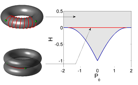
Figure 1: (Color Online) Image of the energy-momentum map $\mathcal{F}$ (gray) for the Hamiltonian of Eq. (15). The singular points are represented by solid blue (black) and red (dark gray) lines. The red line indicates the positions of the image of the bitori (see the text for details). Two trajectories are schematically represented on a regular and on a singular tori (the dots represent the initial and final points of the trajectory). The upper trajectory represents a standard oscillating solution obtained with the energy-minimum cost. The lower trajectory is the ideal adiabatic trajectory, that can not be reached with the energy-minimum cost. Numerical values are taken to be $p_{\rho}=k=1$. The different quantities are unitless in all the figures.

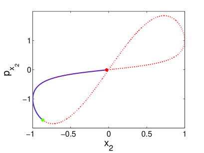
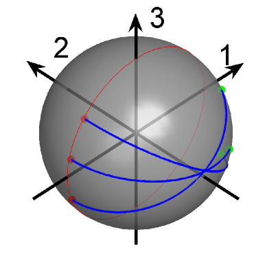
Figure 2: (Color Online) Top: Projection in the $(x_{2},p_{x_{2}})$ plane of a trajectory on the bitorus for $H=0$, $p_{\phi}=0.1$, $p_{\rho}=1$, in the case where $\theta(0)\neq 0$. The parameter $k$ is fixed to 1. Bottom: Projections onto the sphere of different trajectories lying on a bitorus. The green (light gray) and red dots (dark gray) are respectively the initial and final positions of the trajectories. The great circle represents the quantum states with no population in the intermediate level $|2\rangle$.

As mentioned above, a singular reduction [39] allows to make more precise the nature of this singularity (see the appendix A for details). In the energy-momentum diagram depicted in Fig. 1, each point of the horizontal singular line of equation $H=0$ is associated to a bitorus in the phase space, i.e. two tori glued together along a singular circle. Straightforward computations show that the points of this circle satisfy $x_{2}=p_{x_{2}}=0$, i.e. the equation of the STIRAP solution. For comparison, two schematic trajectories on a regular torus and on a bitorus have been plotted in Fig. 1. We notice the difference of structure between these two solutions. The set of all the trajectories belonging to a given bitorus can also be characterized. Two different cases can be distinguished. In the first one, $\theta=\frac{\pi}{2}$, then $p_{\theta}=0$ and the system is on the singular circle which means that no motion is possible. In the second subset, $\theta(t)\neq\frac{\pi}{2}$ at some time $t$, but we observe numerically that the trajectory returns at longer times to the singular circle such that $\theta=\frac{\pi}{2}$. This point is illustrated in Fig. 2.

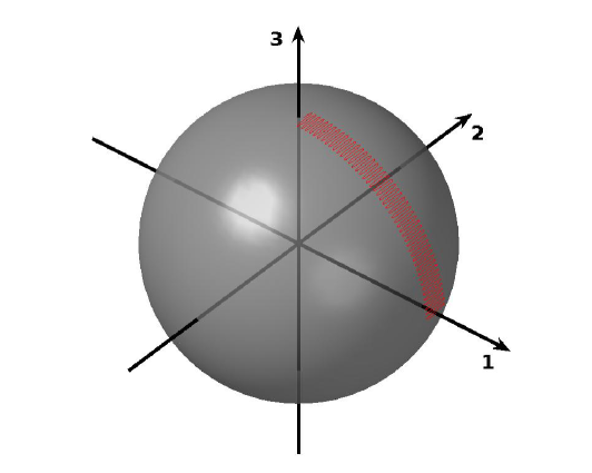
Figure 3: (Color Online) Projection onto the sphere of an optimal trajectory for the energy minimization control problem (top panel) and of the corresponding fields (bottom panel). The pump and the Stokes fields are respectively depicted in blue (black) and in red (dark gray). The parameters are $k=1$ and $T=30$. The values of the adjoint states are $p_{\phi}=15$, $p_{\rho}=69$ and the Hamiltonian $H$ of Eq. (13) is equal to 0.33.

The last step of this preliminary study consists in solving numerically the optimal control problem. For that purpose, we choose some initial values of the momenta $p_{\rho}$, $p_{\theta}$ and $p_{\phi}$ and we propagate the Hamiltonian equations (16) during the time $T$. The distance to the target state is computed at this final time. An example of solution is represented in Fig. 3. Note the oscillatory behavior of the extremal solution, which is far from the expected smooth and monotonic evolution of the adiabatic pulse. These oscillations do not allow to limit the losses from the intermediate state and the final population of the state $|3\rangle$ is only of $0.82$. Such a solution belongs to a regular torus close to the singular one. In spite of this proximity in the energy-momentum diagram, two completely different behaviors are obtained. In addition, a systematic numerical analysis shows that the frequency of the oscillations increases if the control amplitude increases as can be seen in Tab. 1. We observe that the population transfer is better, but the control frequency is larger. On the other hand, if one tries to reduce the oscillatory character of the solution by staying on the singular line or close to it then it is not possible to reach the target state with efficiency, as illustrated by the first line of Tab. 1. We thus conclude that the limit of high energy does not allow to recover the STIRAP process. The other intuitive limit would be a longer control duration, but this is not favorable to STIRAP, as can be seen by comparing the second and third lines of Tab. 1. The STIRAP process is therefore not an intrinsic optimal solution of this problem. A peculiar cost functional has to be chosen in order to highlight the optimal properties of the STIRAP technique.

Table 1: Characteristics of different extremal solutions. The Freq. and Amp. columns indicate respectively a frequency and an amplitude averages of the fields $u_{1}$ and $u_{2}$.

$H$	$p_{\phi}$	$T$	Freq.	Amp.	$C$	$x_{3}^{2}(T)$
0	0.1	4	0	1.7	2.7	$10^{-7}$
0.33	15	30	1.5	1.26	33.9	0.82
0.4	45	8	1.5	4.23	73.6	0.93
4.6	30	10	50	9.81	94.3	0.98

2.4 The STIRAP cost

The study presented above makes clear that the energy minimum cost is not well suited to the STIRAP process. The objective of this section will be to determine a cost, which could force the optimal solution to follow the STIRAP trajectory. From a dynamical point of view, a basic argument is to prevent the Hamiltonian trajectory to curl around a torus. This goal can be achieved by reducing the oscillations around $x_{2}=0$, which leads in spherical coordinates to the cost:

$$C=\int_{0}^{T}\dot{\theta}^{2}dt=\int_{0}^{T}(k\sin\theta\cos\theta+v_{1})^{2}dt.$$ (19)

This choice also avoids populating the state $|2\rangle$ as shown below. The Hamiltonian of the PMP has the form:

$$H=-kr\cos^{2}\theta p_{r}+k\cos\theta\sin\theta p_{\theta}+v_{1}p_{\theta}$$

$$-v_{2}\cot\theta p_{\phi}-\frac{1}{2}(k\sin\theta\cos\theta+v_{1})^{2}.$$

The cost $C$ depending on $v_{1}$ and not on $v_{2}$, we choose to optimize the Hamiltonian $H$ only with respect to $v_{1}$. Optimizing also $v_{2}$ would lead once again to a static solution. We obtain $v_{1}=p_{\theta}-k\sin\theta\cos\theta$ and plugging this expression into the Hamiltonian $H$ gives:

$$H=-krp_{r}\cos^{2}\theta+\frac{1}{2}p_{\theta}^{2}-v_{2}\cot\theta p_{\phi},$$ (20)

where $v_{2}$ is a given time-dependent function. The equations of motion become:

$$\left\{\begin{array}[]{rcl}\dot{r}&=&-kr\cos^{2}\theta\\ \dot{\theta}&=&p_{\theta}\\ \dot{\phi}&=&-\cot\theta\,v_{2}\\ \dot{p_{r}}&=&kp_{r}\cos^{2}\theta\\ \dot{p_{\theta}}&=&-2krp_{r}\sin\theta\cos\theta-\frac{p_{\phi}}{\sin^{2}\theta}v_{2}\\ \dot{p_{\phi}}&=&0.\end{array}\right.$$ (21)

From Eq. (21), it is clear that the solution $p_{\theta}(t)=0$ for any time $t$ minimizes the cost $C$. As a consequence, we get that $\theta(t)$ is constant along this trajectory and the expression of the second control field $v_{2}$ comes from $\dot{p}_{\theta}=0$:

$$v_{2}=-\frac{2krp_{r}\sin^{3}\theta\cos\theta}{p_{\phi}}.$$ (22)

Here the functions $rp_{r}$, $p_{\phi}$ and $\theta$ are constants of motion, $v_{2}$ is also constant. Using Eq. (22), one gets the extremum value of $H$, which reads as:

$$H=2krp_{r}\cos^{2}\theta(\sin^{2}\theta-\frac{1}{2}).$$ (23)

The STIRAP solution can be recovered from the limit case $\theta\to\pi/2$. In this limit, we get $H=0$ and $v_{1}\simeq 0$, leading to $u_{1}\cos\phi=u_{2}\sin\phi$ and

$$\frac{u_{2}}{u_{1}}=\frac{x_{1}}{x_{3}},$$ (24)

which is characteristic of a STIRAP sequence.

To numerically solve this control problem, one should also note that there exist some constraints on the initial momenta. Indeed, if we denote by $\tau$ the typical relaxation time, the following condition holds on the final time: $T<<\tau$. As $\tau=\frac{1}{k\cos^{2}\theta}$ and $T=\left|\frac{\pi}{2v_{2}\cot\theta}\right|$, this leads to the relation:

$$|\frac{\pi p_{\phi}}{4rp_{r}\sin^{2}\theta}|\ll 1.$$

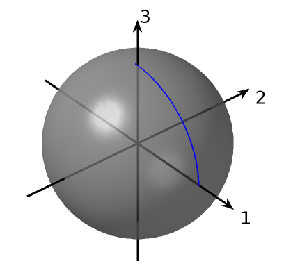
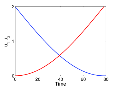
Figure 4: (Color online) Optimal control fields obtained with the Stirap cost (bottom) and the projection of the corresponding trajectory onto the sphere $x_{1}^{2}+x_{2}^{2}+x_{3}^{2}=1$ (top). In the bottom panel, the Stokes and the Pump pulses are respectively depicted in blue (black) and red (gray). Numerical parameters are taken to be $k=1$ and $T=80$. The initial momenta are $p_{\theta}=0$, $p_{\phi}=0.1$, $p_{\rho}=10$. The Hamiltonian $H$ of Eq. (20) is equal to $10^{-3}$.

An example of optimal trajectory is given in Fig. 4. Note the counterintuitive order of the two control fields, one of the main features of a STIRAP process. We can therefore conclude that a STIRAP-like solution can be designed from the PMP if the right cost is considered.

3 Extension to a four-level quantum system

We apply the same reasoning to a four-level quantum system with a tripod structure [37, 40, 41, 42, 43, 7, 33, 34] as illustrated in Fig. 5.

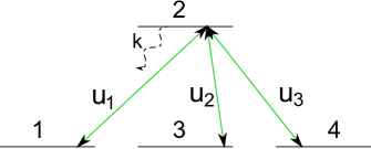
Figure 5: (Color Online) The four-level tripod quantum system. $u_{1}$, $u_{2}$ and $u_{3}$ stand for the pump and the two Stokes pulses respectively. $k$ is the dissipation rate of the second level $|2\rangle$.

The dynamical evolution of this system is described by the Hamiltonian:

$$H=\left(\begin{array}[]{cccc}0&-u_{1}&0&0\\ u_{1}&-ik&-u_{2}&-u_{3}\\ 0&u_{2}&0&0\\ 0&u_{3}&0&0\\ \end{array}\right)$$ (25)

where $u_{1}$, $u_{2}$ and $u_{3}$ stand for the pump and the two Stokes pulses respectively. The aim of the control is to transfer the population of state $|1\rangle$ to a superposition of states $|3\rangle$ and $|4\rangle$, while preventing the system to populate the state $|2\rangle$. We first consider the energy minimization cost $C$ given by

$$C=\frac{1}{2}\int_{0}^{T}[u_{1}^{2}(t)+u_{2}^{2}(t)+u_{3}^{2}(t)]dt.$$ (26)

The pseudo-Hamiltonian of the PMP reads:

$$\begin{array}[]{rcl}H&=&-kx_{2}p_{x_{2}}+u_{1}(x_{1}p_{x_{2}}-x_{2}p_{x_{1}})+u_{2}(x_{2}p_{x_{3}}-x_{3}p_{x_{2}})\\ &&+u_{3}(x_{2}p_{x_{4}}-x_{4}p_{x_{2}})-\frac{1}{2}[u_{1}^{2}(t)+u_{2}^{2}(t)+u_{3}^{2}(t)].\end{array}$$ (27)

Introducing the spherical coordinates:

$$\left\{\begin{array}[]{l}x_{1}=r\cos\theta_{1}\sin\theta_{2}\\ x_{2}=r\cos\theta_{2}\\ x_{3}=r\sin\theta_{1}\sin\theta_{2}\cos\theta_{3}\\ x_{4}=r\sin\theta_{1}\sin\theta_{2}\sin\theta_{3}\end{array}\right.,$$

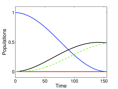
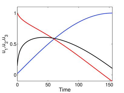
Figure 6: (Color Online) Example of an optimal solution mimicking the adiabatic evolution and leading to a superposition of the states $|3\rangle$ and $|4\rangle$. The top panel depicts the evolution of the population of the different states $|1\rangle$, $|2\rangle$, $|3\rangle$ and $|4\rangle$ respectively in blue (dark gray), red (light gray), black and green (dashed line). In the bottom panel, the Pump, Stokes 1 and Stokes 2 pulses are represented in blue (dark gray), red (light gray) and black, respectively. Numerical values are $p_{\rho}=100,w_{1}=k=1$.

the dynamical system takes the form:

$$\left\{\begin{array}[]{rcl}\dot{r}&=&-kr\cos^{2}\theta_{2}\\ \dot{\theta}_{1}&=&u_{1}\sin\theta_{1}\cot\theta_{2}+u_{2}\frac{\cos\theta_{2}\cos\theta_{1}\cos\theta_{3}}{\sin\theta_{2}}\\ &&+u_{3}\cot\theta_{2}\cos\theta_{1}\sin\theta_{3}\\ \dot{\theta}_{2}&=&k\sin\theta_{2}\cos\theta_{2}-u_{1}\cos\theta_{1}+u_{2}\sin\theta_{1}\cos\theta_{3}\\ &&+u_{3}\sin\theta_{1}\sin\theta_{3}\\ \dot{\theta}_{3}&=&-u_{2}\frac{\cos\theta_{2}\sin\theta_{3}}{\sin\theta_{1}\sin\theta_{2}}+u_{3}\frac{\cos\theta_{2}\cos\theta_{3}}{\sin\theta_{1}\sin\theta_{2}}\end{array}\right..$$ (28)

Using the following rotations on the control fields:

$$\left\{\begin{array}[]{rcl}v_{2}&=&u_{2}\cos\theta_{3}+u_{3}\sin\theta_{3}\\ v_{3}&=&-u_{2}\sin\theta_{3}+u_{3}\cos\theta_{3}\\ \end{array}\right.,$$ (29)

and

$$\left\{\begin{array}[]{rcl}w_{1}&=&u_{1}\sin\theta_{1}+v_{2}\cos\theta_{1}\\ w_{2}&=&-u_{1}\cos\theta_{1}+v_{2}\sin\theta_{1}\\ \end{array}\right.,$$ (30)

the Hamiltonian $H$ becomes:

$$\begin{array}[]{rcl}H&=&-k\,r\cos^{2}\theta_{2}p_{r}+k\cos\theta_{2}\sin\theta_{2}p_{\theta_{2}}+w_{1}\cot\theta_{2}p_{\theta_{1}}\\ &&+w_{2}p_{\theta_{2}}+v_{3}\frac{\cot\theta_{2}}{\sin\theta_{1}}p_{\theta_{3}}-\frac{1}{2}[w_{1}^{2}(t)+w_{2}^{2}(t)+v_{3}^{2}(t)].\end{array}$$ (31)

The analysis of the different Hamiltonian trajectories used in Sec. 2 can be done along the same lines. It can be shown that the Hamiltonian $H$ is integrable since it possesses four constants of the motion: $H$, $L_{1}=x_{3}P_{x_{4}}-x_{4}P_{x_{3}}$, $L_{3}=x_{1}P_{x_{4}}-x_{4}P_{x_{1}}$ and $L_{4}=x_{1}P_{x_{3}}-x_{3}P_{x_{1}}$. Here again, we obtain that the adiabatic trajectory lies on a singular torus in the phase space. In this example, we have to deal with a four dimensional torus in a eight dimensional phase space, which prevents any three dimensional picture. As in the STIRAP case, the optimal solution presents an oscillatory structure in the $\theta_{2}$ variable which is not present in the adiabatic solution. Following the same intuition as in Sec. 2, we give up the minimization of the energy and we choose a cost that allows to minimize the oscillations around $\theta_{2}=\frac{\pi}{2}$:

$$C=\int_{0}^{T}\dot{\theta}_{2}^{2}dt=\int_{0}^{T}(k\sin\theta_{2}\cos\theta_{2}+w_{2})^{2}dt.$$ (32)

Plugging this cost into the Hamiltonian and optimizing with respect to $w_{2}$, which is the only control in the cost, we get:

$$w_{2}=p_{\theta_{2}}-k\sin\theta_{2}\cos\theta_{2},$$

and the Hamiltonian finally reads:

$$\begin{array}[]{rcl}H&=&-krp_{r}\cos^{2}\theta_{2}+\frac{1}{2}p_{\theta_{2}}^{2}+w_{1}\cot\theta_{2}p_{\theta_{1}}\\ &&+v_{3}\frac{\cot\theta_{2}p_{\theta_{3}}}{\sin\theta_{1}}.\end{array}$$ (33)

It is then straightforward to check from the equations of motion that the solution $p_{\theta_{2}}(t)=0$, for any time $t$, minimizes the cost $C$. One deduces that $\theta_{2}$ is constant along this trajectory and we obtain a relation between $v_{3}$ and $w_{1}$ from $\dot{p}_{\theta_{2}}=0$:

$$v_{3}=(2krp_{r}\cos\theta_{2}\,\sin^{3}\theta_{2}-w_{1}p_{\theta_{1}})\frac{\sin\theta_{1}}{p_{\theta_{3}}}.$$ (34)

Hence, by tuning the values of $w_{1}$, which is assumed here to be constant, and of the initial momenta, we can reach any final superposition of the states $|3\rangle$ and $|4\rangle$. For example, by taking $w_{1}=1$, $rp_{r}=100$, $p_{\theta_{1}}(0)=16.85$, $p_{\theta_{2}}(0)=0,p_{\theta_{3}}(0)=-1$, we obtain the same final population in the states $|3\rangle$ and $|4\rangle$ as shown in Fig. 6. Note the counterintuitive order between the pump and the Stokes pulses. The corresponding adiabatic process is associated to the limit $\theta_{2}\to\pi/2$.

4 Conclusion and open questions

We have reached the main goal of this study, which was to exhibit a connection between optimal control theory and adiabatic techniques in quantum systems. A geometric analysis of the Hamiltonian dynamics constructed from the PMP gives a complete overview of all the optimal solutions for a given cost. For the energy minimization problem, we have shown that the adiabatic pulse can be associated to a peculiar Hamiltonian singularity of the problem. The adiabatic solution being a singular Hamiltonian trajectory, it cannot be approached smoothly by any optimal control field. Therefore, an adapted cost functional has to be chosen to enforce the optimal solution to follow the structure of the adiabatic pulse sequence. This study done for three and four level quantum systems is expected to be generalizable to more complex quantum dynamics where an adiabatic control scheme can be used. On the theoretical side, this study is also the first step in the understanding of the role of Hamiltonian singularities in control processes. Although much more work need to be done to advance in this entirely new field, it seems a promising way in order to design optimal control fields with robustness properties. For instance, it would be interesting to apply the same idea to other standard adiabatic processes such as the frequency chirp in a two-level quantum system.

Acknowledgment
We are grateful to H. Yuan for discussions.

Appendix A Singular reduction theory

In this appendix, we apply the singular reduction theory [39] in order to determine the nature of the singular tori presented in Sec. 2. We refer the reader to Ref. [44] for a pedagogical introduction to these tools. Singular reduction theory is a general technique that gives a global overview of all the Hamiltonian trajectories and of the corresponding geometrical structures in which they evolve. This theory is roughly based on the reduction of the dimension of the phase space by making use of a constant of the motion. However, caution should be exercised due to the existence of singularities in the problem. The application of this general procedure to the example of this work can be summarized as follows.

To simplify the analysis, we work on the dynamics projected on the sphere, the constant $r\cdot p_{r}$ playing the role of a parameter. In cartesian coordinates, this leads to the following constraints:

$$x_{1}^{2}+x_{2}^{2}+x_{3}^{2}=1\quad\textrm{and}\quad x_{1}p_{x_{1}}+x_{2}p_{x_{2}}+x_{3}p_{x_{3}}=rp_{r}.$$ (35)

We consider the flow of the constant of motion $p_{\phi}=x_{1}p_{x_{3}}-x_{3}p_{x_{1}}$ to reduce the dimension of the problem. We first introduce the six invariant polynomials under the flow of $p_{\phi}$, which form a basis for the polynomial functions $\mathcal{P}$ which Poisson-commute with $p_{\phi}$, i.e. $\dot{\mathcal{P}}=\left\{\mathcal{P},p_{\phi}\right\}=0$. It is straightforward to check that the following polynomials are invariant [39]:

$$\begin{array}[]{l}\pi_{1}=x_{2}\\ \pi_{2}=p_{x_{2}}\\ \pi_{3}=x_{1}p_{x_{3}}-x_{3}p_{x_{1}}(=p_{\phi})\\ \pi_{4}=p_{x_{1}}^{2}+p_{x_{3}}^{2}\\ \pi_{5}=x_{1}^{2}+x_{3}^{2}\\ \pi_{6}=x_{1}p_{x_{1}}+x_{3}p_{x_{3}}\\ \end{array}$$ (36)

These polynomials obey by construction to the reduced phase space equation:

$$\pi_{6}^{2}+\pi_{3}^{2}=\pi_{4}\pi_{5}.$$ (37)

Since the Hamiltonian $H$ defined in Eq. (15) commutes with $p_{\phi}$, it can be expressed as:

$$H=-k\pi_{1}\pi_{2}+\frac{1}{2}\left(\pi_{1}^{2}\pi_{4}+\pi_{2}^{2}\pi_{5}-2\pi_{1}\pi_{2}\pi_{6}\right)$$ (38)

Using the two constraints of (35), Equations (37) and (39) become:

$$(rp_{r}-\pi_{1}\pi_{2})^{2}+\pi_{3}^{2}=\pi_{4}(1-\pi_{1}^{2}),$$ (39)

and

$$H=-(k+rp_{r})\pi_{1}\pi_{2}+\frac{1}{2}\left(\pi_{1}^{2}\pi_{4}+\pi_{2}^{2}\pi_{1}^{2}+\pi_{2}^{2}\right).$$ (40)

For a given value of $\pi_{3}(=p_{\phi})$, we get two surfaces in the space $(\pi_{1},\pi_{2},\pi_{4})$. The dynamics takes place at their intersection. An example of such intersection is plotted in Fig. 2. This eight-like shape is the mark of a specific type of singular tori, the bitorus which is represented in Fig. 3.

References

- [1] N. V. Vitanov, T. Halfmann, B. Shore and K. Bergmann, Annu. Rev. Phys. Chem. 52, 763 (2001).
- [2] S. Guérin and H. R. Jauslin, Adv. Chem. Phys. 125, 147 (2003).
- [3] M. A. Bernstein, K. F. King and X. J. Zhou, Handbook of MRI Pulse Sequences, Elsevier, Burlington-San Diego-London, 2004.
- [4] M. Shapiro and P. Brumer, Principles of quantum control of molecular processes (Wiley, New York, 2003).
- [5] S. Rice and M. Zhao, Optimal control of molecular dynamics (Wiley, New York, 2003).
- [6] U. Gaubatz, P. Redecki, S. Schiemann and K. Bergmann, J. Chem. Phys. 92, 5363 (1990)
- [7] B. W. Shore, K. Bergmann, J. Oreg and S. Rosenwaks, Phys. Rev. A 44, 7442 (1991)
- [8] R. C. C. Brif and H. Rabitz, New J. Phys. 12, 075008 (2010).
- [9] H. Rabitz, R. de Vivie-Riedle, M. Motzkus and K. Kompa, Science 288, 824 (2000).
- [10] U. Boscain, G. Charlot, J.-P. Gauthier, S. Guérin and H.R. Jauslin, J. Math. Phys. 43, 5 (2002)
- [11] U. Boscain and P. Mason, J. Math. Phys. 47, 062101 (2006).
- [12] B. Bonnard and D. Sugny, SIAM J. on Control and Optimization, 48, 1289 (2009)
- [13] B. Bonnard, M. Chyba and D. Sugny, IEEE Transactions on Automatic control, 54, 11, 2598 (2009)
- [14] N. Khaneja, R. Brockett and S. J. Glaser, Phys. Rev. A, 63, 032308 (2001)
- [15] D. Sugny, C. Kontz and H. R. Jauslin, Phys. Rev. A 76, 023419 (2007)
- [16] M. Lapert, Y. Zhang, M. Braun, S. J. Glaser and D. Sugny, Phys. Rev. Lett. 104, 083001 (2010)
- [17] W. Zhu, J. Botina and H. Rabitz, J. Chem. Phys. 108, 1953 (1998); I. I. Maximov, J. Salomon, G. Turinici and N. C. Nielsen, J. Chem. Phys. 132, 084107 (2010); M. Lapert, R. Tehini, G. Turinici and D. Sugny, Phys. Rev. A 78, 023408 (2008)
- [18] N. Khaneja, T. Reiss, C. Kehlet, T. Schulte-Herbrüggen and S. J. Glaser, J. Magn. Reson. 172, 296 (2005); T. E. Skinner, T. O. Reiss, B. Luy, N. Khaneja and S. J. Glaser, J. Magn. Reson. 167, 68 (2004).
- [19] L. Pontryagin et al., Mathematical theory of optimal processes, Mir, Moscou, 1974.
- [20] B. Bonnard and M. Chyba, Singular trajectories and their role in control theory, Springer SMAI, Vol. 40, 2003.
- [21] V. Jurdjevic, Geometric control theory, Cambridge University Press, Cambridge, 1996.
- [22] T. E. Skinner, T. O. Reiss, B. Luy, N. Khaneja and S. J. Glaser, J. Magn. Reson. 163, 8 (2003).
- [23] T. Hornung, S. Gordienko, R. de Vivie-Riedle and B. J. Verhaar, Phys. Rev. A 66, 043607 (2002).
- [24] X.-Y. Zhang, Z.-R. Sun, G.-L. Chen, Z.-G. Wang, Z.-Z. XÜ, R.-X. Li, Chin. Phys. Lett. 21, 1930 (2004).
- [25] V. S. Malinovsky and D. J. Tannor, Phys. Rev. A 56, 4929 (1997).
- [26] I. R. Sola, V. S. Malinovsky and D. J. Tannor, Phys. Rev. A 60, 3081 (1999).
- [27] Y. B. Band and O. Magnes, J. Chem. Phys. 101, 7528 (1994)
- [28] N. Wang and H. Rabitz, J. Chem. Phys. 104, 1173 (1996)
- [29] Z. Kis and S. Stenholm, J. Mod. Opt. 49, 111 (2002)
- [30] D. Sugny, M. Ndong, D. Lauvergnat, Y. Justum and M. Desouter-Lecomte, J. Photochem. Photobiol. A : Chemistry 190, 359-371 (2007).
- [31] D. Sugny, C. Kontz, M. Ndong, Y. Justum, G. Dive and M. Desouter-Lecomte, Phys. Rev. A 74, 043419 (2006); D. Sugny and M. Joyeux, J. Chem. Phys. 112, 31 (2000).
- [32] H. Yuan, C. P. Koch, P. Salamon and D. J. Tannor, Phys. Rev. A 85, 033417 (2012).
- [33] N. V. Vitanov, B. W. Shore and K. Bergmann, Eur. Phys. J. D 4, 15 (1998)
- [34] T. Nakajima, Phys. Rev. A 59, 559 (1999)
- [35] N. V. Vitanov and S. Stenholm, Phys. Rev. A 56, 1463 (1997)
- [36] P. A. Ivanov, N. V. Vitanov and K. Bergmann, Phys. Rev. A 70, 063409 (2004)
- [37] C. Lazarou and N. V. Vitanov, Phys. Rev. A 82, 033437 (2010)
- [38] V. I. Arnold, Mathematical Methods of Classical Mechanics (Springer-Verlag, New York, 1989).
- [39] R. H. Cushman and L. M. Bates, Global Aspects of Classical Integrable Systems (Birkhauser, Berlin, 1997)
- [40] R. G. Unanyan, B. W. Shore and K. Bergmann, Phys. Rev. A 59, 2910 (1999)
- [41] R. G. Unanyan, M. E. Pietrzyk, B. W. Shore and K. Bergamnn, Phys. Rev. A 70, 053404 (2004)
- [42] D. Moller, L. B. Madsen and K. Molmer, Phys. Rev. A 75, 062302 (2007)
- [43] D. Moller, L. B. Madsen and K. Molmer, Phys. Rev. A 77, 022306 (2008)
- [44] E. Assémat, A. Picozzi, H. R. Jauslin and D. Sugny, J. Opt. Soc. Am. B 29, No. 4, 559 (2012)