Spin-charge conversion in multiterminal Aharonov-Casher ring coupled to precessing ferromagnets: A charge conserving Floquet-nonequilibrium Green function approach

Abstract

We derive a non-perturbative solution to the Floquet-nonequilibrium Green function (Floquet-NEGF) describing open quantum systems periodically driven by an external field of arbitrary strength of frequency. By adopting the reduced-zone scheme, we obtain expressions rendering conserved charge currents for any given maximum number of photons, distinguishable from other existed Floquet-NEGF-based expressions where, less feasible, infinite number of photons needed to be taken into account to ensure the conservation. To justify our derived formalism and to investigate spin-charge conversions by spin-orbit coupling (SOC), we consider the spin-driven setups as reciprocal to the electric-driven setups in S. Souma et. al., Phys. Rev. B 70, 195346 (2004) and Phys. Rev. Lett. 94, 106602 (2005). In our setups, pure spin currents are driven by the magnetization dynamics of a precessing ferromagnetic (FM) island and then are pumped into the adjacent two- or four-terminal mesoscopic Aharonov-Casher (AC) ring of Rashba SOC where spin-charge conversions take place. Our spin-driven results show reciprocal features that excellently agree with the findings in the electric-driven setups mentioned above. We propose two types of symmetry operations, under which the AC ring Hamiltonian is invariant, to argue the relations of the pumped/converted currents in the leads within the same or between different pumping configurations. The symmetry arguments are independent of the ring width and the number of open channels in the leads, terminals, and precessing FM islands, In particular, net pure in-plane spin currents and pure spin currents can be generated in the leads for certain setups of two terminals and two precessing FM islands with the current magnitude and polarization direction tunable by the pumping configuration, gate voltage covering the two-terminal AC ring in between the FM islands.

I Introduction

In this section, we first give the introduction to the phenomenon and effects that motivate our investigation in Sec. I.1. An overview of the attempts of and findings in our study is given in Sec. I.2 where the organization of this paper is also provided.

I.1 Spin pumping, inverse spin-Hall effect, and Aharonov-Casher effect without dc bias voltage

The spin-Hall effect (SHE) is a phenomenon where longitudinal injection of a conventional unpolarized charge current into a system with either extrinsic (due to impurities D’yakonov and Perel’ (1971); Hirsch (1999)) or intrinsic (due to band structure Murakami et al. (2003); Sinova et al. (2004)) spin-orbit coupling (SOC) generates a transverse pure spin current in the four-terminal geometry or the corresponding spin accumulation along the lateral edges in the two-terminal geometry. While the magnitude of the pure spin current generated by SHE in metals and semiconductors is rather small and difficult to control, Awschalom and Flatté (2007) the inverse spin-Hall effect Hirsch (1999); Hankiewicz et al. (2005) (ISHE) has recently emerged as the principal experimental tool to detect induction of pure spin currents by different sources.

In the ISHE (which can be viewed Hirsch (1999); Hankiewicz et al. (2005) as the Onsager reciprocal phenomenon of the direct SHE), a longitudinal spin current generates a transverse charge current or voltage in an open circuit. Experimental examples employing ISHE to detect pure spin current include: (i) a pure spin current pumped by precessing magnetization of a single ferromagnetic (FM) layer under ferromagnetic resonance (FMR) conditions with detection by injecting the pumped current into an adjacent normal-metal (NM), such as Pt, Pd, Au, and Mo, or semiconductor layer; Saitoh et al. (2006); Mosendz et al. (2010) (ii) spin currents generated in nonlocal spin valves; Valenzuela and Tinkham (2006) (iii) a transient ballistic pure spin current injected Werake et al. (2011) by a pair of laser pulses in GaAs multiple quantum wells being converted into a charge current generated by ISHE before the first electron-hole scattering event, thereby providing unambiguous evidence for the intrinsic direct and inverse SHE.

The spin pumping Tserkovnyak et al. (2005) by precessing magnetization is a phenomenon where the moving magnetization of a single FM layer, driven by microwave radiation under the FMR, emits spin current into adjacent NM layers. The emitted spin current is pure in the sense that it is not accompanied by any net charge flux. This effect is termed pumping because it occurs in the absence of any dc bias voltage. Particularly, the detection of pure spin currents pumped by magnetization dynamics has become a widely employed technique Mosendz et al. (2010) to characterize the effectiveness of the charge-spin conversion by the SHE via measuring the material-specific spin-Hall angle (i.e., the ratio of spin-Hall and charge conductivities). The same ISHE-based technique is almost exclusively used in the very recent observations of thermal spin pumping and magnon-phonon-mediated spin-Seebeck effect. Uchida et al. (2011) Also, spin pumping makes it possible to inject Ando et al. (2011) spins into semiconductors with electrically tunable efficiency across an Ohmic contact, evading the notorious problem Rashba (2000) of impedance mismatch between the FM conductor and high-resistivity material.

On the theoretical side, the mechanisms for converting pumped pure spin current into charge current, due to a region with intrinsic or extrinsic SOC into which the pumped spin current is injected, have been analyzed in a number of recent studies. For example, Ref. Ohe et al., 2008 has shown that both transverse and longitudinal charge currents are generated in the four-terminal Rashba-spin-split two-dimensional electron gases (2DEGs) of square shape which is adjacent to the FM island with precessing magnetization that pumps longitudinal pure spin current into the 2DEG. In this scheme, the output charge current can be increased by increasing the strength of the Rashba SOC in the 2DEG.

Furthermore, the recent alternative description Takeuchi et al. (2010) of spin pumping in FM$|$NM multilayers, which encompasses both the earlier considered Silsbee et al. (1979) nonlocal diffusion of the spin accumulation at the FM$|$NM interface generated by magnetization precession and the effective field described by the “standard model” Tserkovnyak et al. (2005) of spin pumping viewed as an example of adiabatic quantum pumping that is captured by the Brouwer scattering formula, Brouwer (1998) has shown that spin-charge conversion does not always occur and that the conversion depends sensitively on the type of spin-orbit interactions. That is, unlike in FM$|$NM systems where spin-charge conversion is driven by the extrinsic SOC and assumed to follow simple phenomenological prediction $\mathbf{j}_{c}\propto\mathbf{S}\times\mathbf{j}_{s}$ ($\mathbf{j}_{c}$ is charge current density, $\mathbf{S}$ is the spin polarization direction, and $\mathbf{j}_{s}$ is the injected spin current density), the pumped charge currents in Rashba systems were found to deviate from this naive formula.

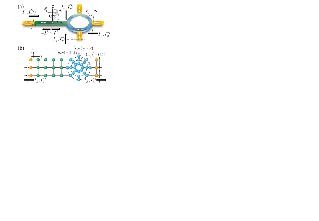
Figure 1: (Color online) Schematics of the (a) four- and (b) two-terminal device setups. A precessing ferromagnetic (FM) island driven by microwaves pumps pure spin current into the Aharonov-Casher (AC) ring (where the spin-charge conversion takes place) patterned within a two-dimensional electron gas in the $x$-$y$ plane with the Rashba spin-orbit coupling. The semi-infinite normal-metal (NM) leads, in the absence of any dc bias voltage, are attached to the AC ring to probe the output time-averaged (over a precession period) pumped charge (spin-$q$ with $q\in\{x,y,z\}$) currents, $I_{L}$ ($I_{L}^{S_{q}}$), $I_{B}$ ($I_{B}^{S_{q}}$), $I_{R}$ ($I_{R}^{S_{q}}$), and $I_{T}$ ($I_{T}^{S_{q}}$), in the left, bottom, right, and top of the device, respectively. The FM island is of length $L_{FM}$, and exchange splitting $\Delta$. The magnetization of the FM precesses around the $z$-axis with frequency $\omega$ and cone angle $\Theta$. The AC ring whose lattice sites along the tangential and normal directions are denoted by $n$ and $m$, respectively.

Thus, the whole phenomenon of spin-charge conversion after pure spin current is injected into a system with SOC needs to be discussed together with the origin of spin currents and the type of SOC employed for the conversion. Takeuchi et al. (2010) Here we analyze spin current generation by one or two precessing FM islands and the corresponding spin-charge conversion in two- and four-terminal mesoscopic rings, adjacent to those islands and patterned in the 2DEG with the Rashba SOC. Unlike the spin-charge conversion in experimental and theoretical studies discussed above, where electronic transport in semiclassical nature, Takeuchi et al. (2010) the device depicted in Fig. 1 involves spin-sensitive quantum-interference effects caused by the difference in the Aharonov-Casher (AC) phase Aharonov and Casher (1984); Mathur and Stone (1992); Richter (2012) gained by a spin traveling around the phase-coherent ring. The AC effect, Aharonov and Casher (1984); Mathur and Stone (1992); Richter (2012) in which magnetic dipoles travel around a tube of electric charge, can be regarded as a special case of a geometric phase. For typical ring sizes and strengths of Rashba SOC in InAlAs/InGaAs heterostructures, the AC phase acquired by a (spin) magnetic moment moving in the presence of an electrical field is of Aharonov-Anandan Aharonov and Anandan (1987) (rather than Berry) type due to the fact that the electron spin cannot Richter (2012) adiabatically maintain a fixed orientation with respect to the radial effective (momentum-dependent and, therefore, inhomogeneous) magnetic field associated with the Rashba SOC. In fact, the AC phase for spins traveling around the mesoscopic ring consists of not only the geometric phase, but also a dynamical phase arising from the additional spin precession driven by the local effective magnetic field. Frustaglia et al. (2004)

Accordingly, giving electrons such geometric phase makes it possible to manipulate the magnitude of charge and spin currents in AC rings due to the fact that, unlike usual case of intrinsically fixed phases, the ring experiments allow one to steer geometric phases in a controlled way through the system geometry and other various tunable parameters. Nagasawa et al. (2012) For example, the destructive quantum interferences, controlled by the accumulated AC phase via tuning of the strength of the Rashba SOC (which depends on the applied top-gate voltage Nitta et al. (1997); Grundler (2000)), cause unpolarized charge current injected into the two-terminal AC rings to diminish König et al. (2006); Nitta and Bergsten (2007); Nagasawa et al. (2012); Frustaglia and Richter (2004); Molnar et al. (2004); Souma and Nikolić (2004) [to zero Souma and Nikolić (2004) if the ring is strictly one-dimensional (1D)]. Similarly, in four-terminal AC rings one encounters quantum-interference-controlled SHE, predicted in Ref. Souma and Nikolić, 2005 and extended to different types of SOC and ring geometry in Refs. Tserkovnyak and Brataas, 2007 and Borunda et al., 2008, where spin-Hall conductance can be tuned from zero to a finite value of the order of spin conductance quantum $e/4\pi$.

I.2 Methodology and key results

The goal of this study is threefold: (i) to provide a unified microscopic quantum transport theory based on the non-perturbative solution of the time-dependent nonequilibrium Green function (NEGF) in the Floquet representation Tsuji et al. (2008) which conserves charge current at each level of approximation (i.e., number of microwave photons taken into account depending on the strength of the driving field) for both the spin current generation by the magnetization dynamics and spin-charge conversion in the adjacent region with SOC; (ii) to understand how output spin and charge currents from multiterminal AC ring device (such as in Fig. 1) can be controlled by the top-gate covering the ring, by the cone angle of precessing magnetization set by the input microwave power driving the precession, and by the setup geometry; (iii) to examine if the device setup in Fig. 1 can be used as a new playground for experiments Richter (2012); König et al. (2006); Nitta and Bergsten (2007); Nagasawa et al. (2012) measuring charge currents to detect quantum interference effects involving AC phase in a single mesoscopic ring where multichannel effects in a typical ring of finite width act as effective dephasing (by entangling spin and orbital degrees of freedom Nikolić and Souma (2005) or averaging over orbital channels with different interference patterns Souma and Nikolić (2004)), thereby randomizing interference patterns as in conventional measurements using dc bias voltage. König et al. (2006)

The paper is organized as follows. In Sec. II, we specify our pumping device and the adopted Hamiltonian. Section III formulates the solution to the Floquet-NEGF equations. Our numerical results are discussed in Sec. IV according to the chosen parameters and units given in Sec. IV.1. In Sec. IV.2, we examine both the pumped charge and spin currents responsible for the AC phase and ISHE effects and driven by spin-pumping in the absence of any dc bias voltage, i.e., the spin-driven setups as the counterparts to the conventional voltage-bias driven (electric-driven) setups with two-terminal Frustaglia and Richter (2004); Molnar et al. (2004); Souma and Nikolić (2004) and four-terminal Souma and Nikolić (2005) mesoscopic AC rings of the Rashba SOC. Section IV.4 illustrates different pumping symmetries of the AC ring. We conclude in Sec. V.

Our key results are as follows: (i) To arrive at Eqs. (32), (33), (34), and (35), we solve the Floquet-NEGF equations and use the so-called reduced-zone scheme Tsuji et al. (2008) which guarantees conservation of charge currents for any given maximum number of photons, unlike other recent approaches based on continued-fraction solutions Martinez (2003); Kitagawa et al. (2011); Wang et al. (2003); Hattori (2008) where charge conservation is ensured only in the limit of infinite number of photons. (ii) With Fig. 2 through Fig. 7, we analyze the pumped currents in the spin-driven setup Fig. 1. The results are in good correspondences to the reciprocal electric-driven results shown in Refs. Souma and Nikolić, 2004 and Souma and Nikolić, 2005, justifying the derived formalism herein. Detail examinations, based on the AC effect and ISHE, of the modulations of both the pumped charge and spin currents are given. (iii) In Sec. IV.4, we tailor the pumping symmetry under which the Hamiltonian of the AC ring of Rashba SOC remains invariant. By performing the symmetry operations on one specific pumping configuration, we can obtain the relations between pumped currents in the same or different pumping configurations (or setup geometry). Although we illustrate the symmetry operations by considering only the setups of two-terminal two-precessing FM islands, the symmetry arguments are applicable to the case of arbitrary number of terminals and FM islands as well, giving multifarious manipulations of the pumped currents via setup geometry. In particular, Fig. 10, Fig. 11, and Fig. 14 through Fig. 17 show that the pumped spin currents are pure and are of magnitude and polarization direction tunable by the top gate voltage controlling the strength of the Rashba SOC and by the pumping configurations.

II Device setup and Hamiltonian

Consider the spin-driven four-terminal (or four-lead) setup in Fig. 1(a). A ferromagnet, FM, with precession axis along the $z$ direction contacts the AC ring of Rashba SOC in the $x$-$y$ plane from the left. The FM plays the role of a spin-$z$ source, pumping pure spin-$z$ currents into the ring via the FM$|$AC-ring interface. The spin-charge conversion takes place in the AC ring. The pumped or converted charge current $I_{p}$ and spin current $I_{p}^{S_{q}}$ are probed by the NM leads where currents are conserved with $p=$ $L$, $R$, $B$, and $T$ indicating the currents flowing through the left, right, bottom, and top leads and $q\in\left\{x,y,z\right\}$ standing for the pumped spin-$x$, $y$, and $z$ currents, respectively.

All computed pumped spin and charge currents are time-averaged (over one precession period); they carry positive signs if the flow direction is in $+x$ or $+y$ direction or minus if flow direction is in $-x$ or $-y$. In the two-terminal setup, Fig. 1(b), we have two NMs labeled by $p=$ $L$, $R$. Note that, except the number of leads, Fig. 1(b) does not differ from Fig. 1(a), but just further shows the lattice structure of the device. The AC ring is modeled by $m=1\cdots M$ concentric circles of the same number of lattice sites, and in a circle $m$ the lattice sites are indexed by $n=1\cdots N$. For instance, we have $(M,N)=(3,8)$ in Fig. 1(b). The NMs and the FM are modeled by square lattices, while each NM is of semi-infinite length, and the FM is of finite length, namely, an island.

The Hamiltonian of the whole device can be divided into six terms,

$$H\left(t\right) = H_{\text{ACR}}+H_{\text{NM}}+H_{\text{FM}}\left(t\right)$$ (1)

$$+H_{\text{NM-ACR}}+H_{\text{FM-ACR}}+H_{\text{FM-NM}}\text{,}$$

where $H_{\text{ACR}}$, $H_{\text{NM}}$, and $H_{\text{FM}}$ account for the Hamiltonian of the AC ring, NM, and FM, respectively. The term $H_{\text{NM-ACR}}$ describes the hybridization between NMs and AC ring, and $H_{\text{FM-ACR}}$ ($H_{\text{FM-NM}}$), the hybridization between FM and AC ring (FM and NMs). Note that the time-dependent Hamiltonian originates only from the precessing FM, $H_{\text{FM}}\left(t\right)$. Below, we express these six terms explicitly.

Focus on $H_{\text{ACR}}$ first. As given in Ref. Souma and Nikolić, 2004, the ring Hamiltonian can be written as,

$$H_{\text{ACR}} = \left[\sum_{\sigma,\sigma^{\prime}=\uparrow,\downarrow}\right.\varepsilon^{n,m}\hat{a}_{n,m;\sigma}^{\dagger}\hat{a}_{n,m;\sigma}$$ (2)

$$-\left(\sum_{n=1}^{N}\sum_{m=1}^{M}\gamma_{\phi}^{n,n+1,m;\sigma,\sigma^{\prime}}\hat{a}_{n,m;\sigma}^{\dagger}\hat{a}_{n+1,m;\sigma^{\prime}}\right.$$

$$\left.-\left.\sum_{n=1}^{N}\sum_{m=1}^{M-1}\gamma_{r}^{m,m+1,n;\sigma,\sigma^{\prime}}\hat{a}_{n,m;\sigma}^{\dagger}\hat{a}_{n,m+1;\sigma^{\prime}}\right)\right]$$

$$+\text{H.c.,}$$

with $n$ and $m$ denoting the lattice sites along the tangential ($\phi$) and normal ($r$) directions as illustrated in Fig. 1(b), respectively. The creation (annihilation) operator at site $(n,m)$ of spin $\sigma$ is $\hat{a}_{n,m;\sigma}^{\dagger}$ ($\hat{a}_{n,m;\sigma}$). The on-site potential $\varepsilon^{n,m}$ at site $(n,m)$ takes into account the disorder and can be tuned by applying a top-gate voltage. In what follows, unless further specified, we will assume that the AC ring, NM, and FM, are all clean conductors, i.e., of zero on-site potentials. The hopping along the $\phi$ direction,

$$\gamma_{\phi}^{n,n+1,m} = \frac{1}{\left(r_{m}/a\right)^{2}\Delta\phi^{2}}\gamma_{0}I_{s}$$ (3)

$$-i\frac{\gamma_{\text{SO}}}{\left(r_{m}/a\right)\Delta\phi}$$

$$\times\left(\sigma_{x}\cos\phi_{n,n+1}+\sigma_{y}\sin\phi_{n,n+1}\right)\text{,}$$

and along the $r$ direction,

$$\gamma_{r}^{m,m+1,n}=\gamma_{0}I_{s}+i\gamma_{\text{SO}}\left(\sigma_{y}\cos\phi_{n}-\sigma_{x}\sin\phi_{n}\right)\text{,}$$ (4)

consists of two terms proportional to $\gamma_{0}$ that originates from the kinetic energy and to $\gamma_{\text{SO}}$ that results from the Rashba SOC, with $\phi_{n}\equiv 2\pi\left(n-1\right)/N$, $\phi_{n,n+1}\equiv\left(\phi_{n}+\phi_{n+1}\right)/2$, $\Delta\phi=\phi_{2}-\phi_{1}$, $r_{m}\equiv r_{1}+\left(m-1\right)a$, $\gamma_{0}=\hbar(2ma^{2})^{-1}$, $\gamma_{\text{SO}}=\alpha\left(2a\right)^{-1},$ $a$ being the lattice spacing, $\sigma_{q}=S_{q}2/\hbar$ being the Pauli matrices, and $\hbar\times 2\pi$, the Planck constant. Being worth addressing, the Hamiltonian (2) yields the same spin precession as obtained by the $SU$(2) non-Abelian spin-orbit gauge Chen and Chang (2008) that absorbs the Rashba SOC term for the U-shaped Liu et al. (2011) 1D conductor; furthermore, the above form of the concentric tight-binding Hamiltonian was also used to theoretically model the Rashba SOC in HgTe/HgCdTe quantum wells in Ref. König et al., 2006, showing experimental observations of the AC effect in good agreements with the theoretical predictions, and thus strengthening the validity of the ring Hamiltonian Eq. (2).

The currents are probed by the un-biased NM leads whose Hamiltonian reads,

$$H_{\text{NM}}=-\sum_{p}\sum_{\sigma=\uparrow,\downarrow}\sum_{\left\langle\mu,\mu^{\prime}\right\rangle}\gamma_{0}\hat{b}_{\mu;\sigma}^{\left(p\right)\dagger}\hat{b}_{\mu^{\prime};\sigma}^{\left(p\right)}\text{,}$$ (5)

where $\hat{b}_{\mu;\sigma}^{\left(p\right)\dagger}$ is the creation operator and $\hat{b}_{\mu;\sigma}^{\left(p\right)}$ is the annihilation operator in lead $p$ at site $\mu$ of spin $\sigma$. The pure spin currents are pumped by the precessing FM described by,

$$H_{\text{FM}}\left(t\right) = \sum_{\sigma,\sigma^{\prime}=\uparrow,\downarrow}\sum_{\nu}\frac{\Delta}{2}\vec{M}\left(t\right)\cdot\vec{\sigma}\hat{c}_{\nu;\sigma}^{\dagger}\hat{c}_{\nu;\sigma^{\prime}}$$ (6)

$$-\sum_{\sigma=\uparrow,\downarrow}\sum_{\left\langle\nu,\nu^{\prime}\right\rangle}\gamma_{0}\hat{c}_{\nu;\sigma}^{\dagger}\hat{c}_{\nu^{\prime};\sigma}$$

$$= \sum_{\sigma,\sigma^{\prime}=\uparrow,\downarrow}\sum_{\nu}\left[Ve^{i\left(\omega t+\Phi\right)}+V^{\dagger}e^{-i\left(\omega t+\Phi\right)}\right.$$

$$\left.+\frac{\Delta}{2}\cos\Theta\sigma_{z}\right]\hat{c}_{\nu;\sigma}^{\dagger}\hat{c}_{\nu^{\prime};\sigma^{\prime}}$$

$$-\sum_{\sigma=\uparrow,\downarrow}\sum_{\left\langle\nu,\nu^{\prime}\right\rangle}\gamma_{0}\hat{c}_{\nu;\sigma}^{\dagger}\hat{c}_{\nu^{\prime};\sigma}\text{,}$$

with $\vec{M}\left(t\right)=\left[\sin\Theta\cos\left(\omega t+\Phi\right),\sin\theta\sin\left(\omega t+\Phi\right),\cos\Theta\right]$ giving $V=\sin\Theta\left(\sigma_{x}-i\sigma_{y}\right)\Delta/4$. The $\hat{c}_{\nu;\sigma}^{\dagger}$ ($\hat{c}_{\nu;\sigma}$) is the creation (annihilation) operator at site $\nu$ in the FM of spin $\sigma$. The hybridizations between adjacent materials,

$$H_{\text{NM-ACR}}=-\gamma_{0}\sum_{p}\sum_{\sigma=\uparrow,\downarrow}\sum_{\left\langle\mu,n\right\rangle}\hat{b}_{p;i;\sigma}^{\dagger}\hat{a}_{n;\sigma}+\text{H.c.,}$$

$$H_{\text{FM-ACR}}=-\gamma_{0}\sum_{\sigma=\uparrow,\downarrow}\sum_{\left\langle\nu,n\right\rangle}\hat{c}_{j;\sigma}^{\dagger}\hat{a}_{n;\sigma}+\text{H.c.,}$$

and

$$H_{\text{FM-NM}}=-\gamma_{0}\sum_{p}\sum_{\sigma=\uparrow,\downarrow}\sum_{\left\langle\nu,\mu\right\rangle}\hat{c}_{j;\sigma}^{\dagger}\hat{b}_{j;i;\sigma}+\text{H.c.}$$

are set to be of the same strength, namely, $\gamma_{0}$.

III Floquet-nonequilibrium Green function approach for periodically driven open quantum systems

In the devices where spin flip or spin precession is absent, the problem of spin pumping by magnetization dynamics can be greatly simplified by mapping it onto a time-independent one in the frame rotating with the precessing magnetization. Zhang et al. (2003); Hattori (2007); Tserkovnyak et al. (2008); Chen et al. (2009) However, the device in Fig. 1 contains Rashba SOC which causes spin-up to evolve into to spin-down by spin precession, so that the device Hamiltonian transformed in the rotating frame contains time-dependent SOC terms.

In the adiabatic regime $\omega\rightarrow 0$, which is satisfied for pumping by magnetization dynamics since the energy of microwave photons $\hbar\omega$ is much smaller than other relevant energy scales, Mahfouzi et al. (2012) one can employ the Brouwer scattering formula. Brouwer (1998) However, this is numerically very inefficient since all pumped spin and charge currents in devices, where the precessing FM island is coupled to a region with SOC, are time-dependent. Ohe et al. (2008) Thus, one has to compute scattering matrix of the device repeatedly at each time step of a discrete grid covering one period of harmonic external potential in order to find full ac current vs. time dependence and then extract experimentally measured dc component.

The relevant dc component of pumped current can be obtained from approaches which generalize the existing steady-state transport theories, such as the scattering matrix, Moskalets and Büttiker (2002); Wu and Cao (2006) NEGF formalism, Tsuji et al. (2008); Martinez (2003); Arrachea (2005); Foa Torres (2005); Wu and Cao (2008, 2010); Kitagawa et al. (2011)and quantum master equations Wu and Timm (2010) with the help of the Floquet theorem Floquet (1883) valid for periodically driven systems. While the equations of the Floquet-NEGF formalism we adopt here have been used before to study a variety of charge pumping problems in non-interacting Martinez (2003); Arrachea (2005); Foa Torres (2005); Wu and Cao (2008) and interacting electron systems Tsuji et al. (2008); Wu and Cao (2010) or the photon-assisted dc transport, Kitagawa et al. (2011) the key issue is to find a solution to these equations that can capture pumping processes at arbitrary strength (or frequency) of the external time-periodic potential while conserving Mahfouzi et al. (2012) charge currents at each step of analytic or numerical algorithm. For example, the often used continued fraction solution Martinez (2003); Kitagawa et al. (2011); Wang et al. (2003); Hattori (2008) to Floquet-NEGF equations does not Mahfouzi et al. (2012) conserve charge current in the leads, and the key trick we employ below to ensure current conservation is the reduced-zone scheme. Tsuji et al. (2008)

We begin the derivation for the charge-current-conserved Floquet-NEGF solution by noting that the two fundamental objects Haug and Jauho (2007) of the NEGF formalism are the retarded

$$G_{\mathcal{I},\mathcal{J}}^{r}\left(t,t^{\prime}\right)\equiv-\frac{i}{\hbar}u\left(t-t^{\prime}\right)\left\langle\left\{\hat{d}_{\mathcal{I}}\left(t\right),\hat{d}_{\mathcal{J}}^{\dagger}\left(t^{\prime}\right)\right\}\right\rangle$$ (7)

and the lesser

$$G_{\mathcal{I},\mathcal{J}}^{<}\left(t,t^{\prime}\right)\equiv\frac{i}{\hbar}\left\langle\hat{d}_{\mathcal{J}}^{\dagger}\left(t^{\prime}\right)\hat{d}_{\mathcal{I}}\left(t\right)\right\rangle\text{,}$$ (8)

Green functions which describe the density of available quantum states and how electrons occupy those states, respectively. Here $u$ is the unit step function; indices $\{\mathcal{I},\mathcal{J}\}\in\{n,m,\mu,\nu,\sigma\}$and creation $\hat{d}^{\dagger}$ or annihilation operators $\hat{d}\in\left\{\hat{a},\hat{b},\hat{c}\right\}$ are used. For notational convenience, the matrix representation with indices $\{\mathcal{I},\mathcal{J}\}$ will not be written out explicitly below.

The essence of the Floquet-NEGF approach is to treat the time variable $t$ in Eq. (1) as an additional real-space degrees of freedom denoted by $\check{t}$ with considering the auxiliary first-quantized Hamiltonian

$$\check{h}\left(\check{t}\right)=h\left(\check{t}\right)-i\hbar\frac{\partial}{\partial\check{t}}\text{.}$$ (9)

Here $h\left(\check{t}\right)$ is the first-quantization version of our actual or original Hamiltonian (1), i.e., the matrix representation for $h\left(t\right)$ is of elements $h_{\mathcal{IJ}}\left(t\right)$ given by $H\left(t\right)=\sum_{\mathcal{I},\mathcal{J}}\hat{d}_{\mathcal{I}}^{\dagger}\hat{d}_{\mathcal{J}}h_{\mathcal{IJ}}\left(t\right)$. The check-hatted symbol $\check{X}$ is used to remind us that $\check{X}$ is an auxiliary variable or operator but not the actual one.

The Schrödinger equation for $\check{h}\left(\check{t}\right)$ reads,

$$i\hbar\frac{\partial}{\partial t}\check{\psi}\left(\check{t},t\right)=\check{h}\left(\check{t}\right)\check{\psi}\left(\check{t},t\right)\text{,}$$ (10)

while keeping in mind again that only $t$ is the real time variable, but $\check{t}$ is a virtual position variable. It is straightforward to prove that, by assuming the wave function $\check{\psi}\left(\check{t},t\right)$ of the form $\check{\psi}\left(\check{t},t\right)=A\left(\check{t}\right)B\left(t\right)$ in Eq.(10) and then letting $\check{t}\rightarrow t$, the original wave function is recovered,

$$\check{\psi}\left(\check{t}=t,t\right)=\psi\left(t\right)\text{,}$$ (11)

where $\psi\left(t\right)$ obeys our original Schrödinger equation $i\hbar\partial\psi\left(t\right)/\partial t=h\left(t\right)\psi\left(t\right)$. Equation (11) plays the fundamental role in the Floquet-NEGF, since it bridges the two systems, the auxiliary time-independent system described by $\check{h}\left(\check{t}\right)$ and our original system described by $h\left(t\right)$. Accordingly, one can first solve the problems in the time-independent system constructed according to Eq. (9), express physical quantities or functions in terms of $\check{\psi}\left(\check{t},t\right)$, and eventually set $\check{t}\rightarrow t$ to obtain the corresponding physical quantities or functions for our original system.

To illustrate the idea above, consider the retarded Green function as an example. The retarded Floquet Green function $\check{G}^{r}\left(t,t^{\prime};\check{t},\check{t}^{\prime}\right)$ corresponding to our auxiliary system $\check{h}\left(\check{t}\right)$ obeys the equation of motion (EOM),

$$\left[i\hbar\frac{\partial}{\partial t}-\check{h}\left(\check{t}\right)\right]\check{G}^{r}\left(t,t^{\prime};\check{t},\check{t}^{\prime}\right)=\delta\left(t-t^{\prime}\right)\delta_{T}\left(\check{t}-\check{t}^{\prime}\right)$$ (12)

where $\delta_{T}\left(\check{t}-\check{t}^{\prime}\right)$ denotes the Dirac delta function of period $T$. Note that $\check{h}\left(\check{t}\right)$ is time-independent; hence, $\check{G}^{r}\left(t,t^{\prime};\check{t},\check{t}^{\prime}\right)$ depends only on the single time variable $t-t^{\prime}$ via the Fourier transformation

$$\check{G}^{r}\left(t,t^{\prime};\check{t},\check{t}^{\prime}\right)=\int_{-\infty}^{\infty}\frac{dE}{2\pi\hbar}e^{-iE\left(t-t^{\prime}\right)/\hbar}\check{G}^{r}\left(E;\check{t},\check{t}^{\prime}\right)$$ (13)

and can be expanded by the wave functions of the form

$$\check{G}^{r}\left(E;\check{t},\check{t}^{\prime}\right)=\sum_{n_{\text{ph}},m_{\text{ph}}=-\infty}^{\infty}\check{\psi}_{n_{\text{ph}}}\left(\check{t}\right)\left[\frac{1}{\left(E+i\eta\right)I-\check{h}}\right]_{n_{\text{ph}},m_{\text{ph}}}\check{\psi}_{m_{\text{ph}}}^{\ast}\left(\check{t}^{\prime}\right)\text{.}$$ (14)

Here, the notations, identity operator $I$, $\eta\rightarrow 0^{+}$, $\left\{n_{\text{ph}},m_{\text{ph}}\right\}\in$ integers, and $\left(\cdots\right)_{n_{\text{ph}},m_{\text{ph}}}\equiv\int_{-T/2}^{T/2}dt\check{\psi}_{n_{\text{ph}}}^{\ast}\left(\check{t}\right)\left(\cdots\right)\check{\psi}_{m_{\text{ph}}}\left(\check{t}\right)$ are used, and the basis

$$\check{\psi}_{n_{\text{ph}}}\left(\check{t}\right)=\left(T\right)^{-1/2}e^{-in_{\text{ph}}\omega\check{t}}$$ (15)

ensures the periodicity $\check{G}^{r}\left(E;\check{t}+lT,\check{t}^{\prime}+l^{\prime}T\right)$ with $\omega\equiv 2\pi/T$ and $\left\{l,l^{\prime}\right\}\in$ integers. The $\left\{\left[\left(E+i\eta\right)I-\check{h}\right]^{-1}\right\}_{n_{\text{ph}},m_{\text{ph}}}$ in Eq. (14) is evaluated according to the definition (9) of $\check{h}$ via

$$\check{h}_{n_{\text{ph}},m_{\text{ph}}} = \int_{-T/2}^{T/2}d\check{t}\check{\psi}_{n_{\text{ph}}}^{\ast}\left(\check{t}\right)\check{h}\left(\check{t}\right)\check{\psi}_{m_{\text{ph}}}\left(\check{t}\right)$$ (16)

$$= h_{n_{\text{ph}},m_{\text{ph}}}-n_{\text{ph}}\hbar\omega\delta_{n_{\text{ph}},m_{\text{ph}}}\text{,}$$

with $n_{\text{ph}}<0$ ($n_{\text{ph}}>0$) accounting for the absorption (emission) processes of photons, as indicated by the subscript “ph”, and

$$h_{n_{\text{ph}},m_{\text{ph}}} = \int_{-T/2}^{T/2}d\check{t}\check{\psi}_{n_{\text{ph}}}^{\ast}\left(\check{t}\right)h\left(\check{t}\right)\check{\psi}_{m_{\text{ph}}}\left(\check{t}\right)$$ (17)

$$= \frac{1}{T}\int_{-T/2}^{T/2}d\check{t}e^{i\left(n_{\text{ph}}-m_{\text{ph}}\right)\omega\check{t}}h\left(\check{t}\right).$$

Note that here beside the $\left\{\mathcal{I},\mathcal{J}\right\}$ degrees of freedoms, the extra degree of freedom, namely, photon is introduced. The $h_{n_{\text{ph}},m_{\text{ph}}}$ exists in the $\left\{\mathcal{I},\mathcal{J}\right\}\otimes n_{\text{ph}}$ Hilbert space, and thus so does $\check{G}^{r}\left(E;\check{t},\check{t}^{\prime}\right)$. The primary result for the actual (original) retarded Green function (7) is obtained by substituting (14), computed by Eqs. (15), (16), and (17), into Eq. (13), and then replacing $\check{t}$ with $t$ and $\check{t}^{\prime}$ with $t^{\prime}$ in the wave-function-expanded Green function, namely $\left.\check{G}^{r}\left(t,t^{\prime};\check{t},\check{t}^{\prime}\right)\right|_{\check{t}\rightarrow t,\check{t}^{\prime}\rightarrow t^{\prime}}=G^{r}\left(t,t^{\prime}\right)$; nonetheless $G^{r}\left(t,t^{\prime}\right)$ can be further simplified by noting the relation that for $l_{\text{ph}}\in$ integers, one has

$$\left[\frac{1}{\left(E+i\eta\right)I-\check{h}}\right]_{n_{\text{ph}},m_{\text{ph}}+l_{\text{ph}}}=\left[\frac{1}{\left(E+l_{\text{ph}}\hbar\omega+i\eta\right)-\check{h}}\right]_{n_{\text{ph}}-l_{\text{ph}},m_{\text{ph}}}\text{,}$$ (18)

which can be deduced simply from the observations that $\mathcal{M}\equiv$ $\left(E+i\eta\right)I-\check{h}$ is a matrix of infinite size, and that $\left[\left(E+i\eta\right)I-\check{h}\right]_{n_{\text{ph}},m_{\text{ph}}+l_{\text{ph}}}$ and $\left[\left(E+l_{\text{ph}}\hbar\omega+i\eta\right)-\check{h}\right]_{n_{\text{ph}}-l_{\text{ph}},m_{\text{ph}}}$ evaluated according to (16) and (17) are at the same position of $\mathcal{M}$, i.e., the same matrix element of $\mathcal{M}$; therefore, the element at the same matrix position of $\mathcal{M}^{-1}$ implies Eq. (18), a manifestation of the reduced-zone scheme in which the energy $E$ can be reduced to the zone of range $\hbar\omega$. With the help of $\left\{\left[\left(E+i\eta\right)I-\check{h}\right]^{-1}\right\}_{n_{\text{ph}},m_{\text{ph}}}=\left\{\left[\left(E+m_{\text{ph}}\hbar\omega+i\eta\right)-\check{h}\right]^{-1}\right\}_{n_{\text{ph}}-m_{\text{ph}},0}$ [$m_{\text{ph}}=0$ and the re-notation $l_{\text{ph}}\rightarrow m_{\text{ph}}$ in Eq. (18)] and change of variables, $E^{\prime}\equiv E+m_{\text{ph}}\hbar\omega$ and $n_{\text{ph}}^{\prime}\equiv n_{\text{ph}}-m_{\text{ph}}$, the retarded Green function now reads,

$$G^{r}\left(t,t^{\prime}\right) = \left.\check{G}^{r}\left(t,t^{\prime};\check{t},\check{t}^{\prime}\right)\right|_{\check{t}\rightarrow t,\check{t}^{\prime}\rightarrow t^{\prime}}$$ (19)

$$= \frac{1}{T}\int_{-\infty}^{\infty}\frac{dE}{2\pi\hbar}e^{-iE\left(t-t^{\prime}\right)/\hbar}\sum_{n_{\text{ph}},m_{\text{ph}}=-\infty}^{\infty}e^{-in_{\text{ph}}\omega t}e^{im_{\text{ph}}\omega t^{\prime}}\left[\frac{1}{\left(E+i\eta\right)I-\check{h}}\right]_{n_{\text{ph}},m_{\text{ph}}}$$

$$= \delta\left(0\right)\int_{-\infty}^{\infty}\frac{dE^{\prime}}{2\pi\hbar}e^{-iE^{\prime}\left(t-t^{\prime}\right)/\hbar}\sum_{n_{\text{ph}}^{\prime}=-\infty}^{\infty}e^{-in_{\text{ph}}^{\prime}\omega t}\check{G}_{n_{\text{ph}}^{\prime},0}^{r}\left(E^{\prime}\right)\text{,}$$

with $\check{G}_{n_{\text{ph}},m_{\text{ph}}}^{r}\left(E\right)\equiv\left\{\left[\left(E+i\eta\right)I-\check{h}\right]^{-1}\right\}_{n_{\text{ph}},m_{\text{ph}}}=\check{G}_{n_{\text{ph}}-m_{\text{ph}},0}^{r}\left(E+m_{\text{ph}}\hbar\omega\right)$; note that the prefactor $\delta\left(0\right)$ in (19) is due to the cancelation of $m_{\text{ph}}\hbar\omega$ in the exponent, i.e., $\delta\left(0\right)=\left(T\right)^{-1}\sum_{m_{\text{ph}}}1=\left(T\right)^{-1}\sum_{m_{\text{ph}}}e^{-im_{\text{ph}}\hbar\omega\times 0}$, while for physical quantities, this prefactor $\delta\left(0\right)$ is irrelevant; instead, it is the normalized [absence of $\delta\left(0\right)$ in (19)] Green function,

$$\bar{G}^{r}\left(t,t^{\prime}\right) \equiv \int_{-\infty}^{\infty}\frac{dE}{2\pi\hbar}e^{-iE\left(t-t^{\prime}\right)/\hbar}$$ (20)

$$\sum_{n_{\text{ph}}=-\infty}^{\infty}e^{-in_{\text{ph}}\omega t}\check{G}_{n_{\text{ph}},0}^{r}\left(E\right)\text{,}$$

that renders physical observable. One can also verify that the expression (20) satisfies the EOM,

$$\left[i\hbar\frac{\partial}{\partial t}-h\left(t\right)\right]\bar{G}^{r}\left(t,t^{\prime}\right)=\delta_{T}\left(t-t^{\prime}\right)\text{,}$$ (21)

by applying $\int_{-T/2}^{T/2}dt^{\prime}$ to both sides of the above Eq. (21). Comparing the EOMs (12) and (21), one clearly sees that the evolution of $\bar{G}^{r}\left(t,t^{\prime}\right)$ is governed by the actual system $h\left(t\right)$, while $\check{G}^{r}\left(t,t^{\prime};\check{t},\check{t}^{\prime}\right)$ is by the auxiliary system $\check{h}\left(\check{t}\right)$.

The lesser Green function can be obtained in the same manner. The auxiliary lesser Green function obeys the Keldysh integral equation,

$$\check{G}^{<}\left(t,t^{\prime};\check{t},\check{t}^{\prime}\right)=\int_{-\infty}^{\infty}\int_{-\infty}^{\infty}dt_{1}dt_{2}\int_{-T/2}^{T/2}\int_{-T/2}^{T/2}d\check{t}_{1}d\check{t}_{2}\check{G}^{r}\left(t,t_{1};\check{t},\check{t}_{1}\right)\check{\Sigma}^{<}\left(t_{1},t_{2};\check{t}_{1},\check{t}_{2}\right)\check{G}^{a}\left(t_{2},t^{\prime};\check{t}_{2},\check{t}^{\prime}\right)\text{.}$$ (22)

The time-independent $\check{h}\left(\check{t}\right)$ allows $\check{G}^{<}\left(t,t^{\prime};\check{t},\check{t}^{\prime}\right)$ to be expressed in terms of the single time variable $t-t^{\prime}$ of the form,

$$\check{G}^{<}\left(t,t^{\prime};\check{t},\check{t}^{\prime}\right)=\int_{-\infty}^{\infty}\frac{dE}{2\pi\hbar}e^{-iE\left(t-t^{\prime}\right)/\hbar}\check{G}^{<}\left(E;\check{t},\check{t}^{\prime}\right)\text{,}$$ (23)

with $\check{G}^{<}\left(E;\check{t},\check{t}^{\prime}\right)$ being Eq. (22) written in the energy domain,

$$\check{G}^{<}\left(E;\check{t},\check{t}^{\prime}\right)=\int_{-T/2}^{T/2}\int_{-T/2}^{T/2}d\check{t}_{1}d\check{t}_{2}\check{G}^{r}\left(E;\check{t},\check{t}_{1}\right)\check{\Sigma}^{<}\left(E;\check{t}_{1},\check{t}_{2}\right)\check{G}^{a}\left(E;\check{t}_{2},\check{t}^{\prime}\right)\text{.}$$ (24)

Here $\check{G}^{a}\left(E;\check{t},\check{t}^{\prime}\right)=\left[\check{G}^{r}\left(E;\check{t}^{\prime},\check{t}\right)\right]^{\dagger}$ is the advanced Green function, and $\check{\Sigma}^{<}\left(E;\check{t},\check{t}^{\prime}\right)=\left|\gamma_{0}\right|^{2}\check{g}^{<}\left(E;\check{t},\check{t}^{\prime}\right)=\sum_{p}\left|\gamma_{0}\right|^{2}\check{g}^{\left(p\right)<}\left(E;\check{t},\check{t}^{\prime}\right)$ is the lesser self energy accounting for the interactions from all probes with the bare (probes that are free of interacting with the environments) lesser Green function of probe $p$ denoted by $\check{g}^{\left(p\right)<}\left(E;\check{t},\check{t}^{\prime}\right)$. The primary result for the lesser Green function (8) is obtained via $\left.\check{G}^{<}\left(t,t^{\prime};\check{t},\check{t}^{\prime}\right)\right|_{\check{t}\rightarrow t,\check{t}^{\prime}\rightarrow t^{\prime}}=G^{<}\left(t,t^{\prime}\right)$ where $\check{G}^{<}\left(t,t^{\prime};\check{t},\check{t}^{\prime}\right)$ is computed by the Green functions in the time-independent system $\check{h}\left(\check{t}\right)$ according to Eqs. (23) and (24). Similarly, $G^{<}\left(t,t^{\prime}\right)$ can also be further simplified by taking advantages of relation (18) and change of variables. For this simplification, we utilize the Keldysh equation in the energy domain Eq. (24) and the wave-function expansion to obtain the expression of $\check{G}^{<}\left(t,t^{\prime};\check{t},\check{t}^{\prime}\right)$,

$$\check{G}^{<}\left(t,t^{\prime};\check{t},\check{t}^{\prime}\right) = \frac{1}{T}\int_{-\infty}^{\infty}\frac{dE}{2\pi\hbar}e^{-iE\left(t-t^{\prime}\right)/\hbar}\sum_{n_{\text{ph}},m_{\text{ph}}=-\infty}^{\infty}\sum_{k_{\text{ph}},l_{\text{ph}}=-\infty}^{\infty}$$ (25)

$$\times e^{-in_{\text{ph}}\omega\check{t}}\left[\frac{1}{\left(E+i\eta\right)I-\check{h}}\right]_{n_{\text{ph}},k_{\text{ph}}}\sum_{p}\left|\gamma_{0}\right|^{2}\check{g}_{k_{\text{ph}},l_{\text{ph}}}^{\left(p\right)<}\left(E\right)\left[\frac{1}{\left(E-i\eta\right)I-\check{h}^{\dagger}}\right]_{l_{\text{ph}},m_{\text{ph}}}e^{im_{\text{ph}}\omega\check{t}^{\prime}}$$

$$= \frac{1}{T}\int_{-\infty}^{\infty}\frac{dE^{\prime}}{2\pi\hbar}e^{-i\left(E^{\prime}-m_{\text{ph}}\hbar\omega\right)\left(t-t^{\prime}\right)/\hbar}$$

$$\times\sum_{n_{\text{ph}},m_{\text{ph}}=-\infty}^{\infty}e^{-in_{\text{ph}}\omega\check{t}}e^{im_{\text{ph}}\omega\check{t}^{\prime}}\sum_{k_{\text{ph}},l_{\text{ph}}^{\prime}=-\infty}^{\infty}\left[\frac{1}{\left(E^{\prime}-m_{\text{ph}}\hbar\omega+i\eta\right)I-\check{h}}\right]_{n_{\text{ph}},k_{\text{ph}}}$$

$$\times\sum_{p}\left|\gamma_{0}\right|^{2}\check{g}_{k_{\text{ph}},l_{\text{ph}}^{\prime}+m_{\text{ph}}}^{\left(p\right)<}\left(E^{\prime}-m_{\text{ph}}\hbar\omega\right)\left[\frac{1}{\left(E^{\prime}-i\eta\right)I-\check{h}^{\dagger}}\right]_{l_{\text{ph}}^{\prime},0}\text{,}$$

where $\left\{\left[\left(E-i\eta\right)I-\check{h}^{\dagger}\right]^{-1}\right\}_{l_{\text{ph}},m_{\text{ph}}}=\left\{\left[\left(E+m_{\text{ph}}\hbar\omega-i\eta\right)I-\check{h}^{\dagger}\right]^{-1}\right\}_{l_{\text{ph}}-m_{\text{ph}},0}$and change of variables, $E^{\prime}\equiv E+m_{\text{ph}}\hbar\omega$ and $l_{\text{ph}}^{\prime}\equiv l_{\text{ph}}-m_{\text{ph}}$ are used. Note that the original Hamiltonian (5) of the NM probes in our present case is time-independent so that we have the expression, $\left|\gamma_{0}\right|^{2}\check{g}_{n_{\text{ph}},m_{\text{ph}}}^{\left(p\right)<}\left(E\right)=-2i\check{f}_{n_{\text{ph}}}^{\left(p\right)}\left(E\right)\left|\gamma_{0}\right|^{2}\text{Im}\check{g}_{n_{\text{ph}},m_{\text{ph}}}^{\left(p\right)r}\left(E\right)=i\check{f}_{n_{\text{ph}}}^{\left(p\right)}\left(E\right)\check{\Gamma}_{n_{\text{ph}},m_{\text{ph}}}^{\left(p\right)}\left(E\right)$, with the Fermi-Dirac distribution (of Fermi energy $E_{F}$ at zero temperature as the regime we are interested in),

$$\check{f}_{n_{\text{ph}}}^{\left(p\right)}\left(E\right) = \check{f}^{\left(p\right)}\left(E+n_{\text{ph}}\hbar\omega\right)$$ (26)

$$= \lim_{\beta\rightarrow 0}\left[1+e^{\left(E+n_{\text{ph}}\hbar\omega-E_{F}\right)/\beta}\right]^{-1}$$

and

$$\check{\Gamma}_{n_{\text{ph}},m_{\text{ph}}}^{\left(p\right)}\left(E\right)=i\left|\gamma_{0}\right|^{2}\left\{\left[\left(E+i\eta\right)I-\check{h}^{\left(p\right)}\right]^{-1}-\left[\left(E-i\eta\right)I-\check{h}^{\left(p\right)\dagger}\right]^{-1}\right\}_{n_{\text{ph}},m_{\text{ph}}}\text{.}$$ (27)

Here the definition (9) yields $\check{h}^{\left(p\right)}\left(\check{t}\right)=h^{\left(p\right)}-i\hbar\partial/\partial\check{t}$ with $h^{\left(p\right)}$ being the first-quantized version of $H_{\text{NM}}=\sum_{p}h^{\left(p\right)}\hat{b}_{p}^{\dagger}\hat{b}_{p}$, and note again because $H_{\text{NM}}$ in Eq. (5) or $h^{\left(p\right)}$ is time-independent, one has $\left[h^{\left(p\right)}\right]_{n_{\text{ph}},m_{\text{ph}}}=\delta_{n_{\text{ph}},m_{\text{ph}}}\left[h^{\left(p\right)}\right]_{n_{\text{ph}}}$, resulting in $\check{\Gamma}_{n_{\text{ph}},m_{\text{ph}}}^{\left(p\right)}\left(E\right)$ proportional to $\delta_{n_{\text{ph}},m_{\text{ph}}}$, i.e., diagonal, and thus the bare lesser Green functions of NMs are diagonal in photon (or Floquet) space $\check{g}_{n_{\text{ph}},m_{\text{ph}}}^{\left(p\right)<}\left(E\right)=\delta_{n_{\text{ph}},m_{\text{ph}}}\check{g}_{n_{\text{ph}}}^{\left(p\right)<}\left(E\right)$ as well. Moreover, applying the same argument we used to derive Eq. (18) to $\check{g}_{n_{\text{ph}},m_{\text{ph}}}^{\left(p\right)<}\left(E\right)$ evaluated by Eqs. (26) and (27), one deduces,

$$\check{g}_{n_{\text{ph}},m_{\text{ph}}+l_{\text{ph}}}^{\left(p\right)<}\left(E\right)=\check{g}_{n_{\text{ph}}-l_{\text{ph}},m_{\text{ph}}}^{\left(p\right)<}\left(E+l_{\text{ph}}\right)\text{,}$$ (28)

which reflects again the reducible property (energy $E$ can be reduced to the zone of range $\hbar\omega$) that yields the reduced-zone scheme. Using above relation (28) and change of variables, $k_{\text{ph}}^{\prime}\equiv k_{\text{ph}}-m_{\text{ph}}$ and $n_{\text{ph}}^{\prime}\equiv n_{\text{ph}}-m_{\text{ph}}$ in Eq. (25), we arrive at,

$$\check{G}^{<}\left(t,t^{\prime};\check{t},\check{t}^{\prime}\right) = \frac{1}{T}\int_{-\infty}^{\infty}\frac{dE^{\prime}}{2\pi\hbar}e^{-i\left(E^{\prime}-m_{\text{ph}}\hbar\omega\right)\left(t-t^{\prime}\right)/\hbar}\sum_{n_{\text{ph}}^{\prime},m_{\text{ph}}}e^{-i\left(n_{\text{ph}}^{\prime}+m_{\text{ph}}\right)\omega\check{t}}e^{im_{\text{ph}}\omega\check{t}^{\prime}}$$ (29)

$$\times\sum_{k_{\text{ph}}^{\prime},l_{\text{ph}}^{\prime}}\left[\frac{1}{\left(E^{\prime}+i\eta\right)I-\check{h}}\right]_{n_{\text{ph}}^{\prime},k_{\text{ph}}^{\prime}}\sum_{p}\left|\gamma_{0}\right|^{2}\check{g}_{k_{\text{ph}}^{\prime},l_{\text{ph}}^{\prime}}^{\left(p\right)<}\left(E^{\prime}\right)\left[\frac{1}{\left(E^{\prime}-i\eta\right)I-\check{h}^{\dagger}}\right]_{l_{\text{ph}}^{\prime},0}\text{,}$$

The actual lesser Green function can be obtained again via setting $\check{t}\rightarrow t$ and $\check{t}^{\prime}\rightarrow t^{\prime}$ in Eq. (29) and noting that $m_{\text{ph}}\hbar\omega$ in the exponent is canceled out; we thus have $\delta\left(0\right)=\left(T\right)^{-1}\sum_{m_{\text{ph}}}1=\left(T\right)^{-1}\sum_{m_{\text{ph}}}e^{-im_{\text{ph}}\hbar\omega\times 0}$, so that the actual lesser Green function can be written as,

$$G^{<}\left(t,t^{\prime}\right) = \left.\check{G}^{<}\left(t,t^{\prime};\check{t},\check{t}^{\prime}\right)\right|_{\check{t}\rightarrow t,\check{t}^{\prime}\rightarrow t^{\prime}}$$

$$= \delta\left(0\right)\int_{-\infty}^{\infty}\frac{dE^{\prime}}{2\pi\hbar}e^{-iE^{\prime}\left(t-t^{\prime}\right)/\hbar}\sum_{n_{\text{ph}}^{\prime}}e^{-in_{\text{ph}}^{\prime}\omega t}\sum_{k_{\text{ph}}^{\prime},l_{\text{ph}}^{\prime}}$$

$$\times\left[\frac{1}{\left(E^{\prime}+i\eta\right)I-\check{h}}\right]_{n_{\text{ph}}^{\prime},k_{\text{ph}}^{\prime}}\sum_{p}\check{g}_{k_{\text{ph}}^{\prime},l_{\text{ph}}^{\prime}}^{\left(p\right)<}\left(E^{\prime}\right)\left[\frac{1}{\left(E^{\prime}-i\eta\right)I-\check{h}^{\dagger}}\right]_{l_{\text{ph}}^{\prime},0}\text{,}$$

and eventually obtain the normalized lesser Green function,

$$\bar{G}^{<}\left(t,t^{\prime}\right) = \int_{-\infty}^{\infty}\frac{dE}{2\pi\hbar}e^{-iE\left(t-t^{\prime}\right)/\hbar}\sum_{n_{\text{ph}}}e^{-in_{\text{ph}}\omega t}\sum_{k_{\text{ph}},l_{\text{ph}}}$$ (30)

$$\times\left[\frac{1}{\left(E+i\eta\right)I-\check{h}}\right]_{n_{\text{ph}},k_{\text{ph}}}\sum_{p}\left|\gamma_{0}\right|^{2}\check{g}_{k_{\text{ph}},l_{\text{ph}}}^{\left(p\right)<}\left(E\right)\left[\frac{1}{\left(E-i\eta\right)I-\check{h}^{\dagger}}\right]_{l_{\text{ph}},0}\text{.}$$

Physical quantities can be extracted from the actual Green function (30). For instance, the quantum-statistical-averaged occupation number at time $t$ on site $i\in\{n,m,\mu\}$ can be expressed as Tr${}_{\text{s}}\left[\bar{G}_{i,i}^{<}\left(t,t\right)O\right]\hbar/i$, while the bond current from site $i$ to site $j$ reads,

$$J_{i\rightarrow j}\left(t\right) = -\text{Tr}_{\text{s}}\left[\frac{\left\{h_{j,i},O\right\}}{2}\bar{G}_{i,j}^{<}\left(t,t\right)\right.$$ (31)

$$\left.-\frac{\left\{h_{i,j},O\right\}}{2}\bar{G}_{j,i}^{<}\left(t,t\right)\right]\text{,}$$

with $O=I_{s}$ ($O=S_{q}$) for particle (spin $S_{q}$) occupations or currents and $I_{s}$ being the $2\times 2$ identity matrix in the Pauli space; the notation Tr${}_{\text{s}}$ stands for performing the trace in the Pauli space (spin Hilbert space), and the anticommutator $\{A,B\}$ is defined as $AB+BA$. The particle (charge) current

$$I_{p}\left(t\right) = \frac{1}{2\pi\hbar}\sum_{p^{\prime}}\sum_{n_{\text{ph}},m_{\text{ph}}}\int_{E_{F}-\hbar\omega/2}^{E_{F}+\hbar\omega/2}dE\text{Tr}^{\prime}\left[\check{G}^{r}\left(E\right)\check{f}^{\left(p^{\prime}\right)}\left(E\right)\check{\Gamma}^{\left(p^{\prime}\right)}\left(E\right)\check{G}^{a}\left(E\right)\check{\Gamma}^{\left(p\right)}\left(E\right)\right.$$ (32)

$$-\left.\check{G}^{r}\left(E\right)\check{\Gamma}^{\left(p^{\prime}\right)}\left(E\right)\check{G}^{a}\left(E\right)\check{f}^{\left(p\right)}\left(E\right)\check{\Gamma}^{\left(p\right)}\left(E\right)\right]_{n_{\text{ph}},m_{\text{ph}}}e^{-i\left(n_{\text{ph}}-m_{\text{ph}}\right)\omega t}$$

and spin current

$$I_{p}^{S_{q}}\left(t\right) = \frac{1}{4\pi}\sum_{p^{\prime}}\sum_{n_{\text{ph}},m_{\text{ph}}}\int_{E_{F}-\hbar\omega/2}^{E_{F}+\hbar\omega/2}dE\text{Tr}^{\prime}\left[\sigma_{q}\check{G}^{r}\left(E\right)\check{f}^{\left(p^{\prime}\right)}\left(E\right)\check{\Gamma}^{\left(p^{\prime}\right)}\left(E\right)\check{G}^{a}\left(E\right)\check{\Gamma}^{\left(p\right)}\left(E\right)\right.$$ (33)

$$-\left.\check{G}^{r}\left(E\right)\check{\Gamma}^{\left(p^{\prime}\right)}\left(E\right)\check{G}^{a}\left(E\right)\check{f}^{\left(p\right)}\left(E\right)\check{\Gamma}^{\left(p\right)}\left(E\right)\right]_{n_{\text{ph}},m_{\text{ph}}}e^{-i\left(n_{\text{ph}}-m_{\text{ph}}\right)\omega t}$$

probed by lead $p$ are obtained by summing all the bond currents (31) flowing through lead $p$. Note here the notation Tr^′ performs the trace over all degrees of freedom, except photon’s. All the functions within the trace are matrices; for example, the Fermi-Dirac distribution is a matrix, $\check{f}^{\left(p\right)}\left(E\right)=\check{f}_{n_{\text{ph}}}^{\left(p\right)}\left(E\right)\delta_{n_{\text{ph}}\text{,}m_{\text{ph}}}$, computed by (26). The time-averaged currents can then be obtained via $I_{p}\equiv$sign$\left(p\right)\times 2\pi\hbar T^{-1}\int_{-T/2}^{T/2}dtI_{p}\left(t\right)$ and $I_{p}^{S_{q}}\equiv$sign$\left(p\right)\times 4\pi T^{-1}\int_{-T/2}^{T/2}dtI_{p}^{S_{q}}\left(t\right)$ as

$$I_{p} = \text{sign}\left(p\right)\times\sum_{p^{\prime}}\int_{E_{F}-\hbar\omega/2}^{E_{F}+\hbar\omega/2}dE\text{Tr}\left[\check{G}^{r}\left(E\right)\check{f}^{\left(p^{\prime}\right)}\left(E\right)\check{\Gamma}^{\left(p^{\prime}\right)}\left(E\right)\check{G}^{a}\left(E\right)\check{\Gamma}^{\left(p\right)}\left(E\right)\right.$$ (34)

$$-\left.\check{G}^{r}\left(E\right)\check{\Gamma}^{\left(p^{\prime}\right)}\left(E\right)\check{G}^{a}\left(E\right)\check{f}^{\left(p\right)}\left(E\right)\check{\Gamma}^{\left(p\right)}\left(E\right)\right]$$

and

$$I_{p}^{S_{q}} = \text{sign}\left(p\right)\sum_{p^{\prime}}\int_{E_{F}-\hbar\omega/2}^{E_{F}+\hbar\omega/2}dE\text{Tr}\left\{\sigma_{q}\left[\check{G}^{r}\left(E\right)\check{f}^{\left(p^{\prime}\right)}\left(E\right)\check{\Gamma}^{\left(p^{\prime}\right)}\left(E\right)\check{G}^{a}\left(E\right)\check{\Gamma}^{\left(p\right)}\left(E\right)\right.\right.$$ (35)

$$-\left.\left.\check{G}^{r}\left(E\right)\check{\Gamma}^{\left(p^{\prime}\right)}\left(E\right)\check{G}^{a}\left(E\right)\check{f}^{\left(p\right)}\left(E\right)\check{\Gamma}^{\left(p\right)}\left(E\right)\right]\right\}\text{,}$$

with sign$\left(p\right)=1$ for $p\in\left\{R,T\right\}$ and sign$\left(p\right)=-1$ for $p\in\left\{L,B\right\}$. Notice here the appearance of sign$\left(p\right)$ is merely for the sign convenience, positive for right- or up-flowing currents, while negative for left- or down-flowing currents. The prefactor $2\pi\hbar$ ($4\pi$) for $I_{p}$ ($I_{p}^{S_{q}}$) are adopted so that the units of $I_{p}$ and $I_{p}^{S_{q}}$ are the same. In other words, if $I_{p}$ measures the number of charge quanta flowing through the lead $p$ per second, then $I_{p}^{S_{q}}$ measures the number of spins $S_{q}$ quanta flowing through the lead $p$ per second. The trace here now is taken over all degrees of freedom, including photon’s.

We emphasize that, in Eqs. (32), (33), (34), and (35), the reduced-zone scheme Tsuji et al. (2008) such as (18) or (28) is adopted, so that the original integral interval $\left[-\infty,\infty\right]$ over energy $E$ is reduced to $\left[E_{F}-\hbar\omega/2,E_{F}+\hbar\omega/2\right]$, and with this scheme, for any given maximum $n_{\text{ph}}$, charge currents are conserved, namely, $\sum_{p}I_{p}\left(t\right)=0$ or $\sum_{p}$sign$\left(p\right)I_{p}=0$. In principle all integers $n_{\text{ph}}$ should account for transport, i.e., transitions involving any number of photons have to be taken into account, nonetheless when the strength of the time-dependent field is small, only few photons can be absorbed or emitted by electrons near Fermi level, and thus considering transitions between channels of few photons are sufficient enough to get accurate results of currents. In our following calculations, $\left|n_{\text{ph}}\right|\leq 2$ is chosen, since we find $\left|n_{\text{ph}}\right|\leq 2$ and $\left|n_{\text{ph}}\right|\leq 3$ do not yield significantly discernible results.

IV Results and discussion

By Eqs. (34) and (35), we show and examine our numerical results for two- and four-terminal spin-pumping setups with the parameters and units specified in Sec. IV.1. In Sec. IV.2, we first concentrate on the two-terminal case [Fig. 1(b)] to see the counterpart physics shown in Ref. Souma and Nikolić, 2004 and then, in Sec. IV.3, we investigate the four-terminal case [Fig. 1(a)] to unveil the phenomena dual to what were found in Ref. Souma and Nikolić, 2005. Our discussions are restricted to the case of single precessing FM in Secs. IV.2 and IV.3. In Sec. IV.4, we aim at building up the relations between probed currents in the same or different pumping configurations from symmetry perspective; the two presented symmetries yield invariant AC ring Hamiltonian, and the arguments on the relations based on the symmetries are generally capable of setups of arbitrary number of precessing FM islands and terminals. Nevertheless, for demonstration simplicity, below in Sec. IV.5, where our numerical results are shown to be in line with the predictions given by the symmetry arguments, we consider only the two-terminal two-precessing-FM setups.

IV.1 Parameters and units

The following parameters and units are used. All energies are in unit of the hopping energy $\gamma_{0}$, and lengths are in unit of the lattice constant $a$. For brevity, the aspect ratio $1/2$ between the length of FM, $L_{FM}$, and the length of AC ring, $N$, is adopted; for example, in Fig. 1(b), we have $L_{FM}/N=4/8$. Also, the width of FM is set to be the same as the width of NM. The default values of parameters of the precession FM (FMs), the spin splitting strength $\Delta=1$, precession frequency (energy) $\hbar\omega=10^{-3}$, precession cone angle $\Theta=10^{\circ}$, and initial precession phase (azimuthal angle) $\Phi=0^{\circ}$ are chosen. To compare the results of our spin-driven setups with the findings of the electric-driven setups in Refs. Souma and Nikolić, 2004 and Souma and Nikolić, 2005, the size of the AC ring are set similar or according to Refs. Souma and Nikolić, 2004 and Souma and Nikolić, 2005. We refer to the ring of $M=1$ as the strict 1D ring, and $M>1$ as the quasi 1D ring. Note again that the sign convention used here is, positive for right- or up-moving flow and negative for left- or down-moving flow. No bias is applied to any probes for what we consider here are all spin-driven setups. The number of open channels $M_{\text{open}}$ in the leads is adjustable by varying $E_{F}$; referring to Fig. 2 in Ref. Souma and Nikolić, 2004, for leads of width consisting of three lattice sites, one has $M_{\text{open}}=1$ approximately in the interval $E_{F}\in[\pm 3.9,\pm 2]$, $M_{\text{open}}=2$ in $E_{F}\in[\pm 2,\pm 0.5]$, and $M_{\text{open}}=3$ in $E_{F}\in[-0.5,0.5]$.

IV.2 Single precessing FM island attached to two-terminal mesoscopic AC ring

We begin with the two-terminal case of clean AC ring in the spin-driven setup Fig. 1(b). Introducing the dimensionless Rashba SOC strength,

$$Q_{R}\equiv\frac{\gamma_{\text{SO}}N}{\gamma_{0}\pi},$$ (36)

we find in Fig. 2 for $(M,N)=(1,200)$ and Fig. 3 for $(M,N)=(3,200)$ where only one channel is open ($M_{\text{open}}=1$), the pumped spin-$z$ current $I_{R}^{S_{z}}$ probed by the right NM lead is a quasi-periodic function of $Q_{R}$; specifically, for $M_{\text{open}}=1$, by increasing $Q_{R}$ the $I_{R}^{S_{z}}$ vanishes at certain $Q_{R}^{\ast}$s, namely, the (AC-spin-interference-induced) modulation nodes; this behavior is akin to the electric-driven setup where the charge current disappears at these $Q_{R}^{\ast}$s.Souma and Nikolić (2004); Frustaglia and Richter (2004); Molnar et al. (2004)

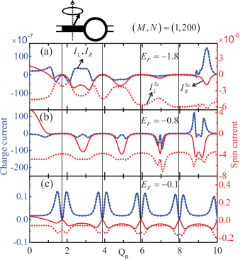
Figure 2: (Color online) Pumped charge and spin currents as a function of the dimensionless Rashba spin-orbit coupling strength $Q_{R}$ in the two-terminal spin-driven setup (top schematics) with ring size $(M,N)=(1,200)$ at different Fermi energies (a) $E_{F}=-1.8$, (b) $E_{F}=-0.8$, and (c) $E_{F}=-0.1$. The ring is in contact with two semi-infinite one-dimensional leads in which currents are probed. The solid vertical lines here indicate the current modulation nodes $Q_{R}^{\ast}$s at which the complete destructive interferences for spin-$z$ take place, causing $I_{R}=I_{R}^{S_{z}}=0$. Since charge currents are conserved, $I_{L}=I_{R}$ is satisfied. The spin-driven results here correspond to the electric-driven results, Fig. 3 in Ref.  Souma and Nikolić, 2004.

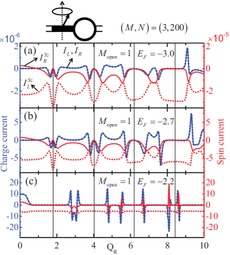
Figure 3: (Color online) Pumped charge and spin currents as a function of the dimensionless Rashba spin-orbit coupling strength $Q_{R}$ in the two-terminal spin-driven setup (top schematics) at different Fermi energies (a) $E_{F}=-3.0$, (b) $E_{F}=-2.7$, and (c) $E_{F}=-2.2$ that yield the number of open channels, $M_{\text{open}}=1$. The ring is of size $(M,N)=(3,200)$ and in contact with two semi-infinite probes of width consisting of three lattice sites. The solid vertical lines here indicate the current modulation nodes $Q_{R}^{\ast}$s. The spin-driven results here correspond to the electric-driven results, Fig. 5 in Ref.  Souma and Nikolić, 2004.

The $I_{R}^{S_{z}}$ modulation originates from the fact that a spin-$z$ acquires some AC phase induced by the Rashba SOC when passing through the AC ring, and the phase difference between the upper-arm and lower-arm of the ring depends on the Rashba SOC strength; accordingly, gradually varying the Rashba SOC strength modulates the spin-$z$ current. The condition of $M_{\text{open}}=1$ is satisfied when $M=1$ (Fig. 2), or when $M>1$ (Fig. 3) with the Fermi energy $E_{F}$ only crossing one subband of the leads. In the former (strict 1D), $Q_{R}^{\ast}$s are independent of the Fermi energy $E_{F}$, while in the latter (quasi 1D), when one tunes $E_{F}$ but keeps $E_{F}$ in the regime $M_{\text{open}}=1$, $Q_{R}^{\ast}$s also remains unaffected (independent of $E_{F}$ as long as $M_{\text{open}}=1$ is satisfied), mimicking again the electric-driven setup. Moreover, since the spin-$z$ current $I^{S_{z}}$ pumped by the FM is pure, if the spin-$z$ encounters a complete destructive interference, i.e., not able to transport through the ring, then no charge currents will be generated in the right NM as well, providing that no passage of spins with different polarizations such as spin-$x$ or spin-$y$ occur through the interface between the right NM and AC ring as we will address below. We refer this types of nodes the AC-spin-interference-induced modulation nodes where $I_{R}^{S_{z}}=0$ and $I_{R}$ vanish concurrently at the same $Q_{R}^{\ast}$s, as indicated by the solid vertical lines in Figs. 2 and 3.

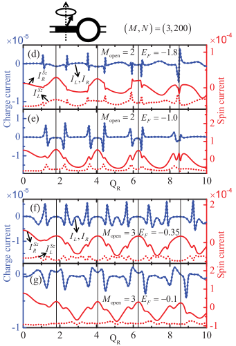
Figure 4: (Color online) Pumped charge and spin currents as a function of the dimensionless Rashba spin-orbit coupling strength $Q_{R}$ in the spin-driven setup same as considered in Fig. 3, while different Fermi energies are chosen to have the number of open channels, $M_{\text{open}}=2$ for (d) $E_{F}=-1.8$ and (e) $E_{F}=-1.0$ and $M_{\text{open}}=3$ for (f) $E_{F}=-0.35$ and (g) $E_{F}=-0.1$. Unlike (a), (b), and (c) with $M_{\text{open}}=1$ in Fig. 2, the modulation here becomes incomplete (absence of the AC-spin-interference-induced modulation nodes at which one has $I_{R}=I_{R}^{S_{z}}=0$, namely, absence of $Q_{R}^{\ast}$s) due to the loss of $M_{\text{open}}=1$, while the (incomplete) quasi-periodicity can still be found as depicted by the solid vertical lines. The spin-driven results here correspond to the electric-driven results, Fig. 6 in Ref. Souma and Nikolić, 2004.

Note that when a pumped spin-$z$ enters the ring, it starts to precess, and there are chances for this spin to become spin-$x$ or spin-$y$ when leaving the ring to the right NM, so that nonzero charge current $I_{R}\neq 0$ without spin-$z$ current $I_{R}^{S_{z}}=0$ can be detected by the right NM. For $I_{R}^{S_{z}}=0$ nodes involving processes as mentioned above are not the AC-spin-interference-induced modulation nodes $Q_{R}^{\ast}$s as being focused here, because they originate from precession but not interference. Noteworthily, although the 1D ring $(M=1)$ in Fig. 2 and quasi-1D ring in Fig. 3 are both in the $M_{\text{open}}=1$ regime, there is an essential difference between them. In Fig. 2, there are no evanescent modes, while in Fig. 3, there are two $(M-M_{\text{open}}=3-1)$ channels that contribute to the evanescent modes; the $Q_{R}^{\ast}$ nodes in Fig. 3 are thus slightly modified from Fig. 2. Also, the $I_{L}^{S_{z}}$ can be nonzero at these $Q_{R}^{\ast}$s, simply because the FM pumps also spin-$z$ currents directly to the left lead. To see the corresponding electric-driven results, compare Fig. 2 here with Fig. 3 in Ref. Souma and Nikolić, 2004 and Fig. 3 here with Fig. 5 in Ref. Souma and Nikolić, 2004.

For $M_{\text{open}}>1$, the conducting spin states become incoherent or impure due to the entanglements between spin and orbit degrees of freedom.Souma and Nikolić (2004) The concept of ensemble average or spin density matrix has to be introduced to describe the transport of interferences induced by the AC effect. Furthermore, when more channels are open, the detected spin phase is obtained by taking into account the transport processes within and between each single channels, and each transport process gives different AC phases yielding different interference nodes (places where the complete destructive interference occurs); thereby, the overall complete destructive interference is washed out by different transport processes, forming the “incomplete” modulations (absence of $Q_{R}^{\ast}$ nodes); for example, in Fig. 4 for $M_{\text{open}}=2$ and $M_{\text{open}}=3$ with $N=200$, although one can still find the quasi-periodicity as depicted by the solid vertical lines, $I_{R}$ and $I_{R}^{S_{z}}$ in general do not vanish concurrently. In addition, some of the pumped spins can be reflected in the FM$|$AC-ring interface before entering the AC ring, so that one has $\left|I_{L}^{S_{z}}\right|\gtrsim\left|I_{R}^{S_{z}}\right|$. To see the electric-driven case corresponding to Fig. 4, compare Fig. 4 here with Fig. 6 in Ref. Souma and Nikolić, 2004. Note that all the above two-terminal results preserve the conservation of charge currents with $I_{L}=I_{R}$.

IV.3 Single precessing FM island attached to four-terminal mesoscopic AC ring

In the four-terminal setup Fig. 1(a), both ISHE and AC effects emerge, giving the inverse quantum-interference-controlled SHE. As shown in Fig. 5 with the ring size $(M,N)=(1,100)$, four semi-infinite 1D probes, and $E_{F}=-0.05$, the transverse currents obey $I_{B}^{S_{z}}=-I_{T}^{S_{z}}$ and $I_{B}=I_{T}$ for all $Q_{R}$, signifying the ISHE. Figure 5 also shows the longitudinal currents in this four-terminal and the corresponding two-terminal setups. In the two-terminal setup, again, because of $M_{\text{open}}=1$, the modulation nodes $Q_{R}^{\ast}$s where $I_{R}$ and $I_{R}^{S_{z}}$ vanish are found, rendering the complete interference modulation. In the four-terminal setup, at these $Q_{R}^{\ast}$s, although $I_{R}$ and $I_{R}^{S_{z}}$ vanish as well, while the longitudinal currents, $I_{L}$ and $I_{L}^{S_{z}}$, do not vanish, and the inequality $I_{L}\neq I_{R}$ shows up due to the presence of the top and bottom leads that break the longitudinal current conservation. Interestingly, the ISHE-induced Hall charge currents $I_{B}=I_{T}$ disappear at these $Q_{R}^{\ast}$s, which demonstrates again the quasi-periodicity of the modulation and is dual (satisfies the Onsager relation) to what was depicted for the SHE-induced Hall spin currents (in the form of spin-Hall conductance) in Fig. 2 of Ref. Souma and Nikolić, 2005. Also note that transverse currents $I_{B}$ and $I_{T}$ decrease as increasing $Q_{R}$ due to the reflections in the interfaces between the AC ring and the top or bottom leads, a manifestation of the lattice Hamiltonian mismatch.

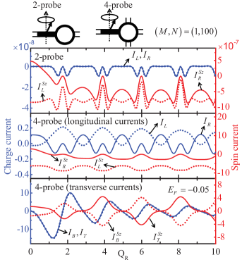
Figure 5: (Color online) Pumped charge and spin currents as a function of the dimensionless Rashba spin-orbit coupling strength $Q_{R}$ in the two-terminal (top panel) and four-terminal (middle and bottom panels) spin-driven setups (see the schematics) in which the same strict one-dimensional ring of size $(M,N)=(1,100)$ is considered. Each of the probes is one-dimensional. The complete modulation nodes $Q_{R}^{\ast}$s that characterize the quasi-periodicity emerge through $I_{R}=I_{R}^{S_{z}}=0$ in both two-and four-terminal setups. In the four-terminal setup, the transverse currents with $I_{B}=I_{T}$ and $I_{B}^{S_{z}}+I_{T}^{S_{z}}=0$ for all $Q_{R}$ reflect the existence of the inverse spin-Hall effect, and the quasi-periodicity can also be identified via $I_{B}=I_{T}=0$ at the same $Q_{R}^{\ast}$s. Note that the Onsager relation is preserved if we compare with the finding in the electric-driven setup, Fig. 2 in Ref.  Souma and Nikolić, 2005.

To see how the width of the ring $M$ affects the interference, we consider the AC ring with fixed $N=100$ in contact with four semi-infinite 1D leads such that only one channel is available for transport in each lead, i.e., $M_{\text{open}}=1$. Figure 6 indicates that the modulation frequency of the Hall currents $I_{B}=I_{T}$ for $M=2$ is almost double to that for $M=1$, because in $M=2$, one additional transport ring path appears. For larger width, the oscillations of Hall currents become vague since the multiple intertwined 1D ring paths smear out the periodic behavior of the currents or average over the AC phase; nevertheless, the complete quasi-periodicity ($I_{B}=I_{T}=0$ at current modulation nodes $Q_{R}^{\ast}$s) is protected by the $M_{\text{open}}=1$ condition. The reciprocal features (for the corresponding electric-driven setup) are shown in Fig. 3 of Ref. Souma and Nikolić, 2005). Note that the ISHE emerging through $I_{B}^{S_{z}}=-I_{T}^{S_{z}}$ and $I_{B}=I_{T}$ is still preserved robustly against the ring width.

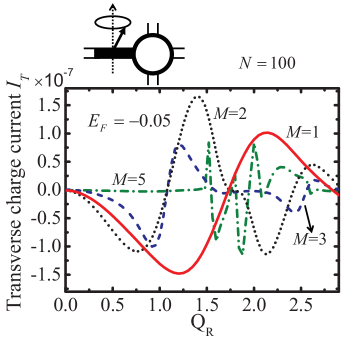
Figure 6: (Color online) Pumped transverse charge currents $I_{T}=I_{B}$ at different ring width $M$ as a function of the dimensionless Rashba spin-orbit coupling strength $Q_{R}$ in the four-terminal spin-driven setup (top schematics) with four semi-infinite one-dimensional probes. Refer to Fig. 3 in Ref. Souma and Nikolić, 2005 for the reciprocal Onsager (electric-driven) results.

Interestingly, the ISHE remains unaffected even in the weak disorder regime. Figure 7 plots the probed currents with different (weak) disorder strength $W$ modeled by the random on-site potentials of the ring, namely, $\varepsilon^{n,m}\in[-W/2,W/2]$. The modulations of $I_{B}^{S_{z}}=-I_{T}^{S_{z}}$ and $I_{B}=I_{T}$ show that ISHE is robust against week disorder. In addition, the presence of the week disorder plays merely the role to reduce the amplitudes of the modulation as also addressed in Ref. Souma and Nikolić, 2005 for the corresponding electric-driven setup (compare Fig. 7 here with Fig. 4 in Ref. Souma and Nikolić, 2005).

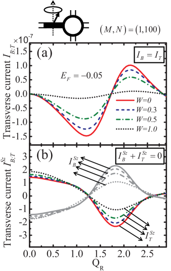
Figure 7: (Color online) Pumped transverse (a) charge and (b) spin-$z$ currents versus the dimensionless Rashba spin-orbit coupling strength $Q_{R}$. The inverse spin-Hall effect (shown through $I_{B}=I_{T}$ and $I_{B}^{S_{z}}+I_{T}^{S_{z}}=0$) survives in the weak disorder regime with different disorder strengths $W$ of the ring in the four-terminal (each of the probes is one-dimensional) spin-driven setup (top schematics). The reciprocal Onsager (electric-driven) result is shown in Fig. 4 of Ref. Souma and Nikolić, 2005.

IV.4 Symmetry operations relating pumped spin and charge currents

We extend our study to the case of multiple precessing FM islands and examine the relations between the pumped currents. Consider the two-terminal setup Fig. 1(b) with an additional FM island inserted between the ring and the right NM (as the schematics shown in Fig. 10). Let $\Theta_{R}$ ($\Theta_{L}$) be the precession cone angle and $\Phi_{R}$ ($\Phi_{L}$) be the initial precession phase of the right (left) FM. For $M_{\text{open}}=1$ at the condition $Q_{R}\approx Q_{R}^{\ast}$, we find that the spin-$z$ currents probed by the left (right) lead remain almost constant when varying $\Theta_{R}$ ($\Theta_{L}$) and/or $\Phi_{R}$ ($\Phi_{L}$); in other words, the left FM does not communicate with the right FM due to the complete destructive interference. Contrarily, in Fig. 8, with $E_{F}=-1.8$, $(M,N)=(1,200)$ ring, two (left and right) 1D leads, fixed $\Theta_{L}=10^{\circ}$ (indicated by the dash line) and $\Phi_{L}=0^{\circ}$ in the left FM, at $Q_{R}=5$, i.e., the condition of the complete destructive interference is off, we see that the pumped currents probed by the left lead, $I_{L}$, $I_{L}^{S_{x}}$, $I_{L}^{S_{y}}$, and $I_{L}^{S_{z}}$, significantly changes with $\Theta_{R}$. For $\Phi_{R}$ dependence, noteworthily, we see that $I_{L}$ and $I_{L}^{S_{z}}$ are not as sensitive to $\Phi_{R}$ as $I_{L}^{S_{x}}$ and $I_{L}^{S_{y}}$ (for example, compare subfigures of Fig. 8 at $\Theta_{R}\approx 135^{\circ}$).

Figure 8: (Color online) Pumped (a) charge current and (b) spin-$x$, (c) spin-$y$, and (d) spin-$z$ currents, in the two-terminal two-precessing-ferromagnet ring device as shown in the schematics of Fig. 10, probed by the left lead as functions of precession cone angle $\Theta_{R}$ and initial precession phase (azimuthal angle) $\Phi_{R}$ of the right ferromagnet. The ring is of size $(M,N)=(1,200)$ and of the dimensionless Rashba spin-orbit coupling strength $Q_{R}=5$. The left ferromagnet is of $\Theta_{L}=10^{\circ}$ (represented by the dash lines) and $\Phi_{L}=0^{\circ}$. The left and right leads are one-dimensional, i.e., the number of open channel $M_{\text{open}}=1$ with Fermi-energy $E_{F}=-1.8$.

To establish a systematic analysis on the relations between pumped currents, we inspect the device from the symmetry perspective. Recall that the Rashba SOC originates from the structural inversion asymmetry,Rashba (1960) meaning that the AC ring Hamiltonian, Eq. (2) defined by Eq. (3) and Eq. (4), does not remain the same by inverting the ring once. This one-time inversion asymmetry, however, leads to the conjecture that if one can somehow perform some inversion-like operations twice, then $H_{\text{ACR}}$ might be invariant. Indeed, at least two types of symmetry operations can render invariant $H_{\text{ACR}}$. These two operations are illustrated in Fig. 9. We refer the first operation as symmetry operation A (abbreviated as SOA), and the second as symmetry operation B (abbreviated as SOB). In SOA, we first invert the system with respect to the $+x$ axis ($x$-inversion) and then invert again with respect to the $+y$ axis ($y$-inversion); note that each inversion gives a $\Delta\phi\rightarrow-\Delta\phi$ and a $\sigma_{z}\rightarrow-\sigma_{z}$. After these two inversions, as shown in Fig. 9 we have, $\phi\rightarrow\pi+\phi$, $\Delta\phi\rightarrow\Delta\phi$, and

$$(\sigma_{x},\sigma_{y},\sigma_{z})\rightarrow(-\sigma_{x},-\sigma_{y},\sigma_{z})\text{, for SOA}$$ (37)

such that Eqs. (3) and (4) remain unaltered, conceding invariant $H_{\text{ACR}}$. For SOB, we first perform the $x$-inversion and then the replacement $(\sigma_{x},\sigma_{y})\rightarrow$ $-(\sigma_{x},\sigma_{y})$; note that in SOB, the $\sigma_{y}$ undergoes $\sigma_{y}\rightarrow-\sigma_{y}\rightarrow\sigma_{y}$ ($\sigma_{y}\rightarrow-\sigma_{y}$ due to the inversion and then $-\sigma_{y}\rightarrow\sigma_{y}$ due to the replacement). We thus get (refer to Fig. 9), $\phi\rightarrow 2\pi-\phi$, $\Delta\phi\rightarrow-\Delta\phi$, and

$$(\sigma_{x},\sigma_{y},\sigma_{z})\rightarrow(-\sigma_{x},\sigma_{y},-\sigma_{z})\text{, for SOB}$$ (38)

so that Eqs. (3) and (4) are unchanged to yield invariant $H_{\text{ACR}}$ as well.

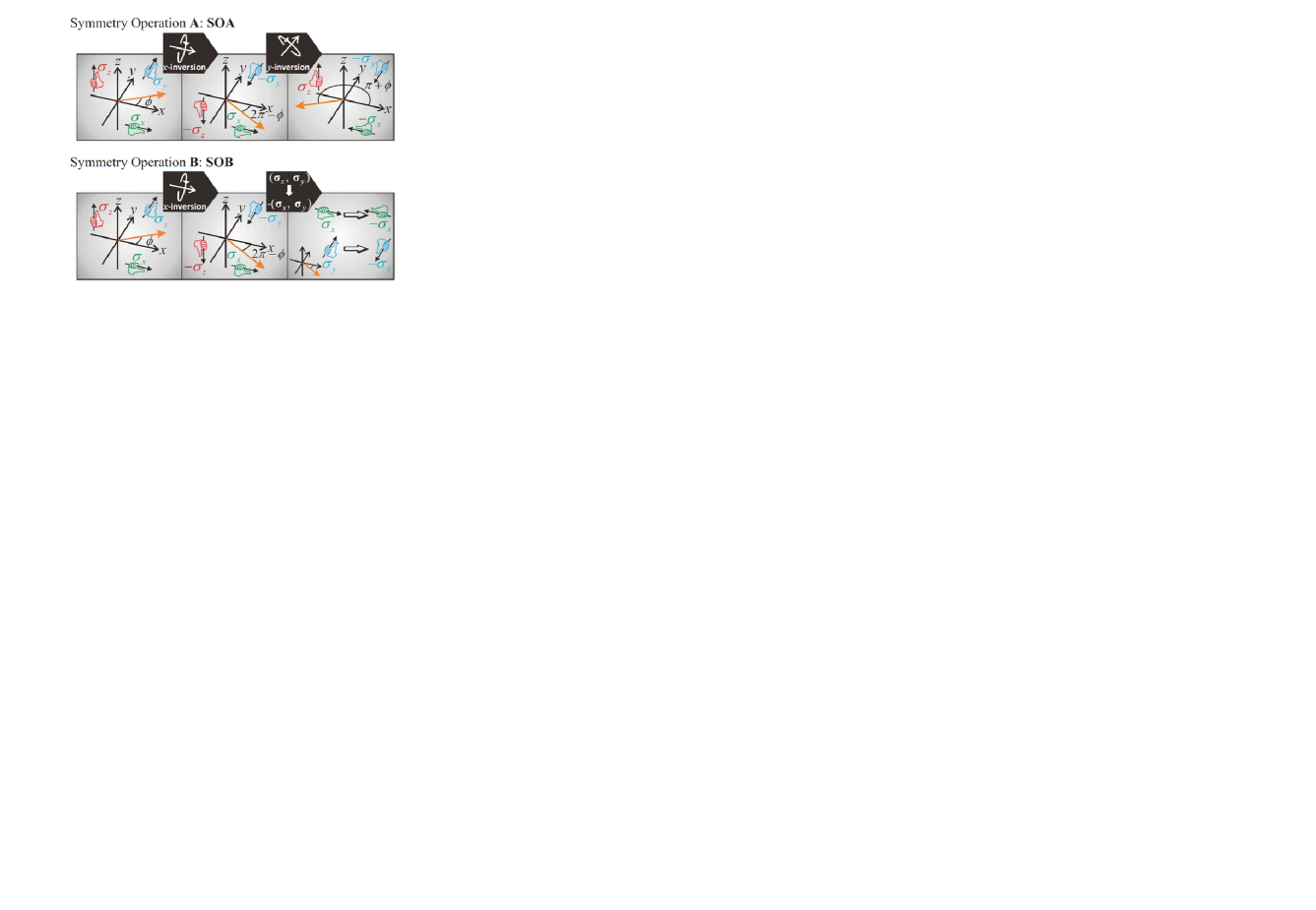
Figure 9: (Color online) Symmetry operations A (SOA) and B (SOB). In SOA, the inversion with respect to the $+x$ axis (as depicted by the inset, $x$-inversion) is first performed to the system represented by the orange/gray arrow lying on the $x$-$y$ plane and then with respect to $+y$ axis (as depicted by the inset, $y$-inversion). In SOB, $x$-inversion is first performed and then the replacement $(\sigma_{x},\sigma_{y})\rightarrow-(\sigma_{x},\sigma_{y})$. The successive figures show how the spin $(\sigma_{x},\sigma_{y},\sigma_{z})$ and polar angle $\phi$ change after each inverting or replacing.

For NMs, obviously, after SOA or SOB, the $H_{\text{NM}}$ remains the same, because all NMs are of the same spin-independent structural-inversion-invariant Hamiltonian. Also, all the hybridizations (characterized by the same spin-independent hopping $-\gamma_{0}$), $H_{\text{NM-ACR}}$, $H_{\text{FM-ACR}}$, and $H_{\text{FM-NM}}$ are SOA- and SOB-invariant. The only portion in the total Hamiltonian that might not be able to recover to its original form is the time-dependent Hamiltonian $H_{\text{FM}}\left(t\right)$, because under SOA or SOB the directions of the precession axis can vary. However, note that since what we are interested in is the time-averaged currents, it is the relative initial precessing phase $\Phi_{L}-\Phi_{R}$ that is relevant to these average currents, while the $\Phi_{L}-\Phi_{R}$ does not change under SOA nor SOB, because SOA or SOB are applied to the whole system (i.e., to all precessing FMs). Moreover, any operations or transformations will transfer one pumping configuration either to the same configuration or to another configuration; in the former, the symmetry argument will relate the probed pumped currents within a single configuration, whereas in the later, relate the probed currents between two different configurations; this will become more clear in the next section. Without loss of generality, in what follows, we choose systems originally at $\Phi_{L}=\Phi_{R}=0^{\circ}$ to illustrate how SOA or SOB helps construct the relations between different probed currents and verify these relations by inspecting our numerical results.

IV.5 Symmetry arguments applied to two precessing FM islands with two-terminal mesoscopic AC ring in between

For the purpose of demonstration, we choose to consider here the two-terminal two-precessing-FM (left and right FMs adjacent to the left and to the right of the ring, respectively) setups, while one can apply the argument presented below also to the ring devices consist of arbitrary number of terminals and precessing FM islands. In addition, since the definitions of SOA and SOB have nothing to do with the ring width $M$, ring length $N$, number of open channels $M_{\text{open}}$, and $E_{F}$, the symmetry argument is valid for any $M$, $N$, $M_{\text{open}}$, and $E_{F}$. Here, we choose $\left(M,N\right)=(3,200)$ and set $E_{F}=-1.8\gamma_{0}$ giving $M_{\text{open}}=2$ to exemplify the symmetry operations. We use the notation convention $A$-$B$ to describe the pumping configuration, with $A$ accounting for the left precessing FM and $B$ for the right precessing FM. Here, with $\{A$, $B\}\in\{P_{\Theta}$, $\bar{P}_{\Theta}\}$, $P_{\Theta}$ ($\bar{P}_{\Theta}$) stands for the FM that is of precession axis along $+z$ ($-z$) axis and of precession cone angle $\Theta$. For example, the schematics in Fig. 10 is notated as $P_{10^{\circ}}$-$P_{10^{\circ}}$, in Fig. 12 as $P_{10^{\circ}}$-$\bar{P}_{10^{\circ}}$, and in Fig. 17 as $\bar{P}_{90^{\circ}}$-$P_{90^{\circ}}$.

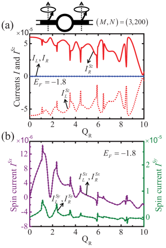
Figure 10: (Color online) Pumped (a) charge and spin-$z$ currents and (b) spin-$x$ and spin-$y$ currents probed by the left and right leads of finite width consisting of three lattice points versus the dimensionless Rashba spin-orbit coupling strength $Q_{R}$ in the two-terminal two-precessing-FM setup $P_{10^{\circ}}$-$P_{10^{\circ}}$ (top schematics), i.e., the left ferromagnet and right ferromagnet are of precession cone angle $10^{\circ}$ and precession axes both along $+z$ direction.

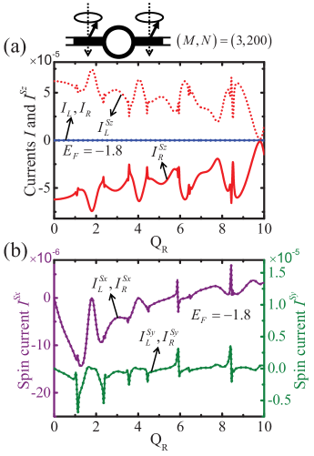
Figure 11: (Color online) Pumped (a) charge and spin-$z$ currents and (b) spin-$x$ and spin-$y$ currents versus the dimensionless Rashba spin-orbit coupling strength $Q_{R}$ in the two-precessing-FM setup $\bar{P}_{10^{\circ}}$-$\bar{P}_{10^{\circ}}$ (top schematics) same as the one considered in Fig. 10 but with precession axes along $-z$ direction for both the left and right ferromagnets.

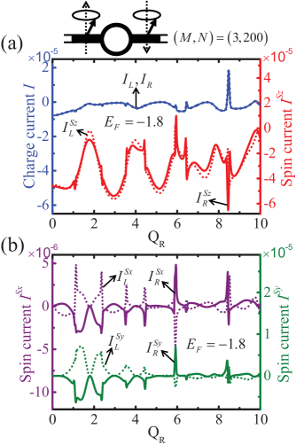
Figure 12: (Color online) Pumped (a) charge and spin-$z$ currents and (b) spin-$x$ and spin-$y$ currents versus the dimensionless Rashba spin-orbit coupling strength $Q_{R}$ in the two-precessing-FM setup $P_{10^{\circ}}$-$\bar{P}_{10^{\circ}}$ (top schematics) same as the one considered in Fig. 10 but with precession axis along $+z$ ($-z$) direction for the left (right) ferromagnet.

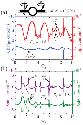
Figure 13: (Color online) Pumped (a) charge and spin-$z$ currents and (b) spin-$x$ and spin-$y$ currents versus the dimensionless Rashba spin-orbit coupling strength $Q_{R}$ in the two-precessing-FM setup $\bar{P}_{10^{\circ}}$-$P_{10^{\circ}}$ (top schematics) same as the one considered in Fig. 10 but with precession axis along $-z$ ($+z$) direction for the left (right) ferromagnet.

Focus on SOA first. Consider $P_{10^{\circ}}$-$P_{10^{\circ}}$, Fig. 10. By applying SOA to $P_{10^{\circ}}$-$P_{10^{\circ}}$, the first step ($x$-inversion) generates $\bar{P}_{80^{\circ}}$-$\bar{P}_{80^{\circ}}$, while the second step ($y$-inversion) yields the swap $L$ (left) $\leftrightarrow R$ (right) and turns $\bar{P}_{80^{\circ}}$-$\bar{P}_{80^{\circ}}$ into $P_{10^{\circ}}$-$P_{10^{\circ}}$, i.e., the original pumping configuration is recovered. As a result, in $P_{10^{\circ}}$-$P_{10^{\circ}}$ we have, due to the $y$-inversion involved in SOA, $I_{L}=-I_{R}$ (or $I_{L}^{S_{q}}=-I_{R}^{S_{q}}$ for all $q$ components before any operations on spins), which then incorporated with the replacement (37) turns $I_{L}^{S_{q}}=-I_{R}^{S_{q}}$ into $(I_{L}^{S_{x}},I_{L}^{S_{y}},I_{L}^{S_{z}})=(I_{R}^{S_{x}},I_{R}^{S_{y}},-I_{R}^{S_{z}})$, in line with our numerical result, Fig. 10. In Fig. 11 ($\bar{P}_{10^{\circ}}$-$\bar{P}_{10^{\circ}}$), by employing the same argument based on SOA, we obtain again the relations $I_{L}=-I_{R}$ and $(I_{L}^{S_{x}},I_{L}^{S_{y}},I_{L}^{S_{z}})=(I_{R}^{S_{x}},I_{R}^{S_{y}},-I_{R}^{S_{z}})$. Being noteworthy, in the pumping configuration $A$-$A$ such as Figs. 10 and 11, the probed charge currents vanish $I_{L}=I_{R}=0$ due to the left-right transmission symmetry,Chen et al. (2009) resulting in pure spin currents in the NMs; this absence of charge currents can also be obtained by noting that the current conservation $I_{L}=I_{R}$ and the symmetry argument that gives $I_{L}=-I_{R}$ have to be satisfied simultaneously.

On the other hand, for the left-right transmission asymmetric cases such as Figs. 12 ($P_{10^{\circ}}$-$\bar{P}_{10^{\circ}}$) and 13 ($\bar{P}_{10^{\circ}}$-$P_{10^{\circ}}$), $I_{L}$ and $I_{R}$ in general can be nonzero. Similarly, performing SOA on $P_{10^{\circ}}$-$\bar{P}_{10^{\circ}}$ ($\bar{P}_{10^{\circ}}$-$P_{10^{\circ}}$), the $x$-inversion renders $\bar{P}_{80^{\circ}}$-$P_{80^{\circ}}$ ($P_{80^{\circ}}$-$\bar{P}_{80^{\circ}}$), and then the proceeding $y$-inversion gives $\bar{P}_{10^{\circ}}$-$P_{10^{\circ}}$ ($P_{10^{\circ}}$-$\bar{P}_{10^{\circ}}$); hence, SOA transfers $P_{10^{\circ}}$-$\bar{P}_{10^{\circ}}$ ($\bar{P}_{10^{\circ}}$-$P_{10^{\circ}}$) to the different pumping configuration $\bar{P}_{10^{\circ}}$-$P_{10^{\circ}}$ ($P_{10^{\circ}}$-$\bar{P}_{10^{\circ}}$). Therefore, the current $I_{L;R}$ in $P_{10^{\circ}}$-$\bar{P}_{10^{\circ}}$ ($\bar{P}_{10^{\circ}}$-$P_{10^{\circ}}$) equals to $-I_{R;L}$ in $\bar{P}_{10^{\circ}}$-$P_{10^{\circ}}$ ($P_{10^{\circ}}$-$\bar{P}_{10^{\circ}}$). Again, the relations above for charge currents together with the replacement (37) make $(I_{L}^{S_{x}},I_{L}^{S_{y}},I_{L}^{S_{z}})$ in $P_{10^{\circ}}$-$\bar{P}_{10^{\circ}}$ ($\bar{P}_{10^{\circ}}$-$P_{10^{\circ}}$) identical to $(I_{R}^{S_{x}},I_{R}^{S_{y}},-I_{R}^{S_{z}})$ in $\bar{P}_{10^{\circ}}$-$P_{10^{\circ}}$ ($P_{10^{\circ}}$-$\bar{P}_{10^{\circ}}$) and $(I_{R}^{S_{x}},I_{R}^{S_{y}},I_{R}^{S_{z}})$ in $P_{10^{\circ}}$-$\bar{P}_{10^{\circ}}$ ($\bar{P}_{10^{\circ}}$-$P_{10^{\circ}}$) identical to $(I_{L}^{S_{x}},I_{L}^{S_{y}},-I_{L}^{S_{z}})$ in $\bar{P}_{10^{\circ}}$-$P_{10^{\circ}}$ ($P_{10^{\circ}}$-$\bar{P}_{10^{\circ}}$). All above features are again in line with our numerical results, Fig. 12 and Fig. 13. It should be noted here that $\Theta=10^{\circ}$ in our numerical calculation is chosen merely for the illustrations of symmetry operations. The symmetry argument presented above in fact is applicable for any cone angle $\Theta$ and even for the case of $\Theta_{L}\neq\Theta_{R}$, i.e., the precessing cone angles for left ($\Theta_{L}$) and right ($\Theta_{R}$) FMs are different. Particularly, at $\Theta=\Theta_{L}=\Theta_{R}=90^{\circ}$, all the relations based on SOA shown above are preserved as well (see Figs. 14, 15, 16, and 17), while since the pumping configuration for $\Theta=90^{\circ}$ (precession within the two-dimensional $x$-$y$ plane) is of higher geometrical symmetry than $\Theta=10^{\circ}$, the probed currents are of additional relations as demonstrated below.

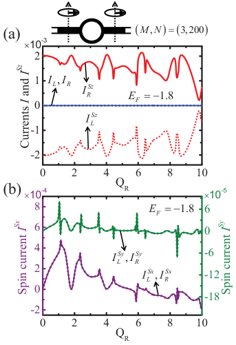
Figure 14: (Color online) Pumped (a) charge and spin-$z$ currents and (b) spin-$x$ and spin-$y$ currents probed by the left and right leads of finite width consisting of three lattice points versus the dimensionless Rashba spin-orbit coupling strength $Q_{R}$ in the two-terminal two-precessing-FM setup $P_{90^{\circ}}$-$P_{90^{\circ}}$ (top schematics), i.e., both the left and right ferromagnets are of precession cone angle $90^{\circ}$ and precession axis along $+z$ direction.

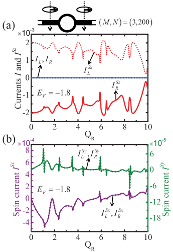
Figure 15: (Color online) Pumped (a) charge and spin-$z$ currents and (b) spin-$x$ and spin-$y$ currents versus the dimensionless Rashba spin-orbit coupling strength $Q_{R}$ in the two-precessing-FM setup $\bar{P}_{90^{\circ}}$-$\bar{P}_{90^{\circ}}$ (top schematics) same as the one considered in Fig. 14 but with precession axis along $-z$ direction for both left and right ferromagnets.

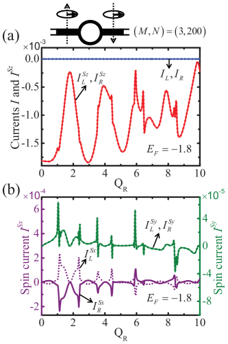
Figure 16: (Color online) Pumped (a) charge and spin-$z$ currents and (b) spin-$x$ and spin-$y$ currents versus the dimensionless Rashba spin-orbit coupling strength $Q_{R}$ in the two-precessing-FM setup $P_{90^{\circ}}$-$\bar{P}_{90^{\circ}}$ (top schematics) same as the one considered in Fig. 14 but with precession axis along $+z$ ($-z$) direction for the left (right) ferromagnet.

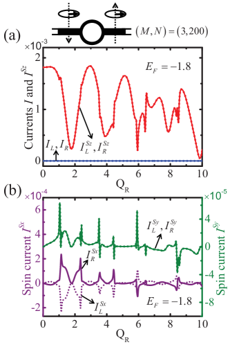
Figure 17: (Color online) Pumped (a) charge and spin-$z$ currents and (b) spin-$x$ and spin-$y$ currents versus the dimensionless Rashba spin-orbit coupling strength $Q_{R}$ in the two-precessing-FM setup $\bar{P}_{90^{\circ}}$-$P_{90^{\circ}}$ (top schematics) same as the one considered in Fig. 14 but with precession axis along $-z$ ($+z$) direction for the left (right) ferromagnet.

Following the same procedure presented above, one can also apply SOB to any $A$-$B$ configuration to relate probed currents in a single pumping configuration (if SOB does not generate another pumping configuration) or to relate probed currents between different pumping configurations (if SOB generates another pumping configuration). Here, we choose to focus on the special case with $\Theta=90^{\circ}$. Unlike the case of $\Theta=10^{\circ}$ where we have no relations of the pumped currents between the two different pumping configurations, $P_{10^{\circ}}$-$P_{10^{\circ}}$ and $\bar{P}_{10^{\circ}}$-$\bar{P}_{10^{\circ}}$, at $\Theta=90^{\circ}$ the pumped currents in $P_{90^{\circ}}$-$P_{90^{\circ}}$ can relate to the pumped currents in $\bar{P}_{90^{\circ}}$-$\bar{P}_{90^{\circ}}$. Applying SOB to $P_{90^{\circ}}$-$P_{90^{\circ}}$ (Fig. 14) yields $\bar{P}_{90^{\circ}}$-$\bar{P}_{90^{\circ}}$ (Fig. 15) so that $I_{L(R)}$ in $P_{90^{\circ}}$-$P_{90^{\circ}}$ is equal to $I_{L(R)}$ in $\bar{P}_{90^{\circ}}$-$\bar{P}_{90^{\circ}}$. This relation, again, incorporated with the replacement (38) leads to the spin current $(I_{L(R)}^{S_{x}},I_{L(R)}^{S_{y}},I_{L(R)}^{S_{z}})$ in $P_{90^{\circ}}$-$P_{90^{\circ}}$ equal to the spin current $(-I_{L(R)}^{S_{x}},I_{L(R)}^{S_{y}},-I_{L(R)}^{S_{z}})$ in $\bar{P}_{90^{\circ}}$-$\bar{P}_{90^{\circ}}$. The above predictions agree with our numerical results, Figs. 14 and 15. Being worth noting, although $P_{10^{\circ}}$-$P_{10^{\circ}}$, $\bar{P}_{10^{\circ}}$-$\bar{P}_{10^{\circ}}$, $P_{90^{\circ}}$-$P_{90^{\circ}}$, and $\bar{P}_{90^{\circ}}$-$\bar{P}_{90^{\circ}}$ all generate net pure in-plane ($x$-$y$ plane) spin currents, i.e., $I_{L}+I_{R}=I_{L}^{S_{z}}+I_{R}^{S_{z}}=0$ as predicted by SOA, the pumped spin currents at $\Theta=90^{\circ}$ are one to two order larger than those at $\Theta=10^{\circ}$ (compare Figs. 10 and 11 with Figs. 14 and 15). Similar enhancement of the pumped spin currents by the cone angle can also be found by comparing Figs. 12 ($P_{10^{\circ}}$-$\bar{P}_{10^{\circ}}$) and 13 ($\bar{P}_{10^{\circ}}$-$P_{10^{\circ}}$) with Figs. 16 ($P_{90^{\circ}}$-$\bar{P}_{90^{\circ}}$) and 17 ($\bar{P}_{90^{\circ}}$-$P_{90^{\circ}}$). The additional (beside what were obtained by SOA) relations between $P_{90^{\circ}}$-$\bar{P}_{90^{\circ}}$ and $\bar{P}_{90^{\circ}}$-$P_{90^{\circ}}$ can be obtained by performing SOB. Applying SOB to $P_{90^{\circ}}$-$\bar{P}_{90^{\circ}}$ (Fig. 16), we arrive at $\bar{P}_{90^{\circ}}$-$P_{90^{\circ}}$ (Fig. 17), with $I_{L(R)}$ in $P_{90^{\circ}}$-$\bar{P}_{90^{\circ}}$ equal to $I_{L(R)}$ in $\bar{P}_{90^{\circ}}$-$P_{90^{\circ}}$, and then, by replacement (38), $(I_{L(R)}^{S_{x}},I_{L(R)}^{S_{y}},I_{L(R)}^{S_{z}})$ in $P_{90^{\circ}}$-$\bar{P}_{90^{\circ}}$ equal to $(-I_{L(R)}^{S_{x}},I_{L(R)}^{S_{y}},-I_{L(R)}^{S_{z}})$ in $\bar{P}_{90^{\circ}}$-$P_{90^{\circ}}$, in line with Figs. 16 and 17. We note that for all $\Theta=90^{\circ}$ pumping configurations, the pumped spin currents are pure (namely, $I_{L}=I_{R}=0$); this again can be achieved by considering the current conservation together with the symmetry argument based on SOA and SOB. We emphasize that our results here show that the current polarization direction can be tuned by the top gate voltage governing $Q_{R}$, and the magnitude of the pumped currents can be controlled by the precession cone angle $\Theta$, offering amenable manipulations on the output currents from the proposed devise.

V Conclusion

In conclusion, by introducing the auxiliary system where the time domain is treated effectively as an additional real-space degree of freedom, we offer a plain access to the Floquet-NEGF formalism capable of dealing with time-periodic dynamic problems in full quantum approach. Particularly, by further adopting the reduced-zone scheme, Tsuji et al. (2008) we derived expressions (32), (33), (34), and (35) in which charge currents are conserved for any given maximum number of photons. With the help of Eqs. (34) and (35), we reveal the physics attributed to the AC effect by considering the ring of Rashba SOC in spin-driven four- [Fig. 1(a)] and two-terminal [Fig. 1(b)] setups.

When the number of open channel in the leads is one, $M_{\text{open}}=1$, as a consequence of the AC effect, the complete AC-spin-interference-induced modulation nodes characterized by $I_{R}=I_{R}^{S_{z}}=0$ at certain Rashba SOC strengths $Q_{R}^{\ast}$s (where the complete destructive interferences occur) are found to be independent of the Fermi energy $E_{F}$ in both two- and four-terminal cases (Figs. 2, 3, and 5).

In the four-terminal setup, the interference modulation is also characterized by $I_{B}=I_{T}=0$ at the corresponding two-terminal $Q_{R}^{\ast}$s (i.e., Fig. 5, top panel $I_{R}=I_{R}^{S_{z}}=0$ and bottom panel $I_{B}=I_{T}=0$ vanish at the same $Q_{R}^{\ast}$s). Increasing the number of open channels by tuning the Fermi-energy to reach $M_{\text{open}}>1$ regime in quasi 1D (of finite width) rings destroys the completeness of the modulation, i.e., absence of $Q_{R}^{\ast}$ (Fig. 4). Nevertheless, in the four-terminal case, we find that the ISHE identified by $I_{B}=I_{T}$ and $I_{B}^{S_{z}}+I_{T}^{S_{z}}=0$ (Fig. 5, bottom panel) is robust against the ring width (Fig. 6) and weak disorder (Fig. 7), and therefore, the proposed device offers a durable electrical means to measure the pure spin currents pumped by the precessing FM islands using the inverse quantum-interference-controlled SHE in the AC rings. The above features based on our spin-driven setups reciprocally well correspond to the findings in the electric-driven setup, Refs. Souma and Nikolić, 2004 and  Souma and Nikolić, 2005, supporting our derived formalism.

In addition to single-precessing-FM setup (Fig. 1), multiple-precessing-FM setup is studied. In the two-terminal two-precessing-FM setup where the ring is in contact with two (left and right) precessing FM islands, we find that the currents probed by the left (right) lead are independent of $\Theta_{R}$ and $\Phi_{R}$ ($\Theta_{L}$ and $\Phi_{L}$) of the right (left) FM under the condition of complete destructive interferences. In other words, the complete destructive interference blocks out the relation between the left portion (left FM and left lead) and the right portion (right FM and right lead) of our device, while this relation revives when the condition of the destructive interference is suppressed (Fig. 8).

We also identified two symmetry operations, SOA and SOB (Fig. 9), to examine the relations between currents in the same pumping configurations or different configurations. Performing SOA or SOB on an arbitrary pumping configuration together with the fact that charge currents should be conserved, one can first relate the charge currents either in the same or in different pumping configurations, and then using Eq. (37) for SOA or Eq. (38) for SOB, one can further obtain the relations between spin currents. We choose to exemplify how the above procedure works by considering the two-terminal two-precessing-FM setup with precession cone angles $\Theta_{L}=\Theta_{R}=10^{\circ}$ (Figs. 10, 11, 12, and 13) and $\Theta_{L}=\Theta_{R}=90^{\circ}$ (Figs. 14, 15, 16, and 17). The relations predicted by SOA and SOB consist with our numerical results. Especially, the net pure in-plane spin currents (for $x$-$y$ plane with $I_{L}+I_{R}=I_{L}^{S_{z}}+I_{R}^{S_{z}}=0$ in Figs. 10, 11, 14, and 15, and for $y$-$z$ plane with $I_{L}+I_{R}=I_{L}^{S_{x}}+I_{R}^{S_{x}}=0$ in Figs. 16 and 17) can be achieved, and for all $\Theta_{L}=\Theta_{R}=90^{\circ}$ pumping configurations, the pumped spin currents are pure, namely, $I_{L}=I_{R}=0$. Therefore, with employing the spin-pumping device proposed here, the pumped currents can be controlled with their magnitudes and polarization directions tunable via the pumping configurations (including the precessing cone angle) and the applied top-gate voltage that varies $Q_{R}$), giving potential applications in spintronics-based industry.