Stochastic Kronecker Graph on Vertex-Centric BSP

Abstract

Recently Stochastic Kronecker Graph (SKG), a network generation model, and vertex-centric BSP, a graph processing framework like Pregel, have attracted much attention in the network analysis community. Unfortunately the two are not very well-suited for each other and thus an implementation of SKG on vertex-centric BSP must either be done serially or in an unnatural manner.

In this paper, we present a new network generation model, which we call Poisson Stochastic Kronecker Graph (PSKG), that generate edges according to the Poisson distribution. The advantage of PSKG is that it is easily parallelizable on vertex-centric BSP, requires no communication between computational nodes, and yet retains all the desired properties of SKG.

1 Introduction

With the advent of massive real-world network data and the computation power to process them, network analysis is becoming a major topic of scientific research. As approaches to model real-world networks, Stochastic Kronecker Graph (SKG) [7] and its predecessor R-MAT [5] have attracted interest in the network analysis community due to its simplicity and its ability to capture many properties of real-world networks. As a programming model to process large graphs, vertex-centric BSP, such as Pregel [8], Apache Giraph [2], GPS [9], and Apache Hama [3], has become increasingly popular as an alternative to MapReduce and Hadoop, which are ill-suited to run massive scale graph algorithms [8].

The two, however, are not well-suited for each other. The obvious approach of parallelizing SKG, which is to generate edges in parallel, is not “vertex-centric” in nature and therefore is unnatural to program and runs inefficiently in vertex-centric BSP.

Therefore we present a new network generation model, which we call Poisson Stochastic Kronecker Graph (PSKG), as an alternative. In this model, the out-degree of each vertex is determined by independent but non-identical Poisson random variables and the destination node of the edges are determined in a recursive manner similar to SKG.

The resulting algorithm, PSKG, is essentially equivalent to SKG and will therefore retain all the desired properties of it. Unlike SKG, however, PSKG is embarrassingly parallel in a vertex-centric manner and therefore is very well-suited for vertex-centric BSP.

Figure 1: Illustration of SKG. At each of the $k$ steps a sub-region is chosen with probability $p_{i,j}$.

2 Theory and Algorithm

The main result of this paper, PSKG, is presented in Algorithm 3. We shall, however, start by discussing the original SKG and an equivalent formulation of it as this path will motivate PSKG. We then present the main algorithm. We conclude this section by discussing issues with load balancing.

Remark.

Throughout this paper we shall use zero-based indexing for vectors and matrices.

2.1 Stochastic Kronecker Graph

Consider the problem of generating a random graph of $E$ edges and $N=n^{k}$ vertices, where $k\in\mathbb{N}$. Let

$$P=\begin{bmatrix}p_{0,0}&\cdots&p_{0,n-1}\\ \vdots&\ddots&\vdots\\ p_{n-1,0}&\cdots&p_{n-1,n-1}\end{bmatrix}\in\mathbb{R}^{n\times n}$$

be the “initiator matrix” where $p_{i,j}\geq 0$ and $\sum_{i,j}p_{i,j}=1$.

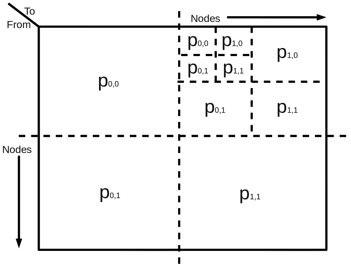
The approach in SKG is to start off with an empty adjacency matrix and “drop” edges into the matrix one at a time. Each edge chooses one of the $n\times n$ partitions with probability $p_{i,j}$ respectively. The chosen partition is again subdivided into smaller partitions, and the procedure is repeated $k$ times until we reach a single cell of the $N\times N$ adjacency matrix and place an edge. Figure 1 illustrates the idea and Algorithm 1 makes it concrete.

Algorithm 1 SKG

  for $i=1,\cdots E$ do

     $u=v=0$

     for $j=1,\cdots k$ do

        With probability $p_{rs}$ choose subregion $(r,s)$

        $u=nu+r;\,v=nv+s$

     end for

     Add edge $(u,v)$

  end for

Let $P_{k}=P\otimes P\otimes\cdots\otimes P$ be the $k$-th Kronecker power of $P$. Then we can interpret SKG as generating $m$ edges independently where any given edge is $(u,v)$ with probability $(P_{k})_{uv}$. Now we can apply Bayes’ rule.

$$\mathbf{P}(\text{edge is }(u,v))=(P_{k}\mathbf{1})_{u}\frac{(P_{k})_{uv}}{(P_{k}\mathbf{1})_{u}}$$ (1)

$$=\mathbf{P}(\text{destination is }u)\mathbf{P}(\text{source is }v|\text{destination is }u)$$

The decomposition (1) permits us to choose the source node first and then the destination node rather than simultaneously and we do this with a recursive algorithm to avoid the explicit construction of $P_{k}$. Let

$$U=\begin{bmatrix}\sum_{j=0}^{n-1}p_{0,j}\\ \vdots\\ \sum_{j=0}^{n-1}p_{n-1,j}\\ \end{bmatrix}\quad V=\begin{bmatrix}\frac{p_{0,0}}{U_{0}}&\cdots&\frac{p_{0,n-1}}{U_{0}}\\ \vdots&\ddots&\vdots\\ \frac{p_{n-1,0}}{U_{n-1}}&\cdots&\frac{p_{n-1,n-1}}{U_{n-1}}\end{bmatrix}$$

and we arrive at Algorithm 2 which is equivalent to the original formulation of SKG.

Algorithm 2 Equivalent SKG

  for $i=1,\cdots E$ do

     //Select source node $u$

     $u=0$

     for $j=1,\cdots k$ do

        With probability $U_{r}$ choose subregion $r$

        $u=nu+r$

     end for

     //Select destination node $v$

     $v=0$; $z=u$

     for $j=1,\cdots k$ do

        $l=\mathrm{mod}(z,n)$

        With probability $V_{ls}$ choose subregion $s$

        $v=nv+s;\,z=z/n$ (integer division)

     end for

     Add edge $(u,v)$

  end for

Here we note that the source node selection procedure is (approximately) a multinomial random variable with parameters $E$ and $U^{[k]}$, where $U^{[k]}$ is the $k$-th Kronecker power of $U$.

2.2 Poisson Stochastic Kronecker Graph

Due to the following elementary result [4] we can replace the source node selection procedure, a multinomial random variable, with i.i.d. Poisson random variables.

Lemma.

Let $X_{1},\cdots X_{s}$ be independent Poisson random variables each with mean $\alpha p_{1},\cdots\alpha p_{s}$, where $\alpha>0$, $p_{1},\cdots p_{s}\geq 0$, and $\sum^{s}_{i=1}p_{i}=1$. Then

$$\mathbf{P}\left(X_{1}=x_{1},\cdots X_{s}=x_{s}\middle|\sum^{s}_{i=1}X_{i}=m\right)$$

$$=\frac{m!}{x_{1}!\cdots x_{s}!}p_{1}^{x_{1}}\cdots p_{k}^{x_{s}}$$

i.e. conditioned on the sum $X_{1},\cdots X_{s}$ is distributed as a multinomial distribution.

We are finally ready to state the main algorithm of this paper. Let $E$ be the expected number of total edges while $P,U,V,k$ are defined the same as before.

Algorithm 3 PSKG

  Scatter $E,P,U,V,k$

  for Each vertex $u$ do

     //Determine out-degree of $u$

     $p=1$; $z=u$

     for $j=1,\cdots k$ do

        $l=\mathrm{mod}(z,n)$; $p=pU_{l}$

        $z=z/n$ (integer division)

     end for

     Generate $X\sim\mathrm{Poisson}(Ep)$

     //For each edge determine destination vertex

     for $i=1,\cdots X$ do

        $v=0$; $z=u$

        for $j=1,\cdots k$ do

           $l=\mathrm{mod}(z,n)$

           With probability $V_{ls}$ choose subregion $s$

           $v=nv+s;\,z=z/n$ (integer division)

        end for

        Add edge $(u,v)$

     end for

  end for

PSKG will retain all the desired properties of SKG graphs. Specifically, say there is a desired property observed by SKG graphs of all sizes with probability $1-\varepsilon$. Then the Poisson SKG graphs will also have the desired property with probability $1-\varepsilon$ by the following lemma.

Lemma.

Let $A$ be an event that occurs with probability $1-\varepsilon$ for SKG graphs of all sizes. Then $A$ will also hold with probability $1-\varepsilon$ for Poisson SKG graphs as well.

Proof.

$$\mathbf{P}_{Poisson}(A)=\mathbf{E}\left[\mathbf{P}\left(A\middle|\sum^{k}_{i=1}X_{i}=m\right)\right]$$

$$=\mathbf{E}\left[\mathbf{P}_{Multinomial}(A|m)\right]>\mathbf{E}[1-\varepsilon]=1-\varepsilon$$

∎

[.1 [.$p_{1}$ [.$p_{1}^{2}$ $p_{1}^{3}=17\%$
$17\%$ $p_{1}^{2}p_{2}=14\%$
$30\%$ ] [.$p_{1}p_{2}$ $p_{1}^{2}p_{2}=14\%$
$44\%$ $p_{1}p_{2}^{2}=11\%$
$55\%$ ] ] [.$p_{2}$ [.$p_{1}p_{2}$ $p_{1}^{2}p_{2}=14\%$
$69\%$ $p_{1}p_{2}^{2}=11\%$
$80\%$ ] [.$p_{2}^{2}$ $p_{1}p_{2}^{2}=11\%$
$91\%$ $p_{2}^{3}=9\%$
$100\%$ ] ] ].1

Figure 2: An example of load balancing where $n=2$, $p_{1}=0.55$, $p_{2}=0.45$, $k=3$, and $N_{\mathrm{w}}=4$. The second to last line denotes the load of each vertex and the last line denotes the cumulative load. The 4 processors attempt to take $25\%$ of the total load each. Consequently processor number 0, 1, 2, and 3 takes ownership to the blue, green, purple, and red vertices, respectively.

2.3 Probabilistic Load Balancing

In vertex-centric BSP, where each computational worker takes ownership to vertices and their outgoing edges, it is not a priori clear how to distribute them; some vertices have more neighbors than others so assigning an equal number to each worker will likely result in load imbalance. As the storage requirement of the graph structure is proportional to the number of neighbors, we shall discuss load balancing with the goal of distributing the number of edges equally.

Let $N_{\mathrm{w}}$ denote the total number of workers to balance the load among and $w_{\mathrm{id}}=0,1,\cdots(N_{\mathrm{w}}-1)$ denote the individual processor number. Let $U^{[k]}$ be the $k$-th Kronecker power of $U$ and $(U^{[k]})_{u}$ the expected load proportion for vertex $u$. Now we split the set of vertices into contiguous partitions (contiguous by node numbering) so that each partition has a total load of about $1/N_{\mathrm{w}}$ and is owned by one processor. This procedure is illustrated in Figure 2.

To do this partitioning efficiently, however, one must avoid explicitly forming $U^{[k]}$. Algorithm 4 achieves this by traversing the decision tree without explicitly forming it.

One legitimate concern of this strategy is that the load is only balanced in expectation and therefore it is possible that with bad luck the actual load is highly unbalanced. However, Theorem 1 tells us that with high probability the load imbalance is small.

Theorem 1.

The $\alpha$-level confidence interval of the maximum load over all computational nodes is $[\frac{E}{N_{\mathrm{w}}},\frac{E}{N_{\mathrm{w}}}+\delta]$ where

$$\delta=\sqrt{\frac{2E}{N_{\mathrm{w}}}}\sqrt{\log N_{\mathrm{w}}+\left|\log\left|\log(1-\alpha)\right|\right|}$$

where $\frac{E}{N_{\mathrm{w}}}$ is the load under perfect balance. We can interpret $\delta$ as the degree of load imbalance.

Proof.

We first make the assumption that the expected load, $E$, is split and distributed perfectly, i.e. each worker will have a load of $X_{i}$ where $X_{0},\cdots X_{N_{\mathrm{w}}-1}$ are i.i.d. Poisson random variables with mean $E/N_{\mathrm{w}}$. Let $M$ be the upper bound of the confidence interval.

$$\mathbf{P}\left(\max_{i}X_{i}\leq M\right)=\mathbf{P}\left(X_{1}\leq M\right)^{N_{\mathrm{w}}}$$

$$=F_{X}^{N_{\mathrm{w}}}(M)\leq 1-\alpha$$

$$M\leq F^{-1}_{X}\left((1-\alpha)^{1/N_{\mathrm{w}}}\right)\approx F^{-1}_{X}\left(1+\frac{\log(1-\alpha)}{N_{\mathrm{w}}}\right)$$

$$\approx\sqrt{\frac{E}{N_{\mathrm{w}}}}\Phi^{-1}\left(1+\frac{\log(1-\alpha)}{N_{\mathrm{w}}}\right)+\frac{E}{N_{\mathrm{w}}}$$

$(1-\alpha)^{1/N_{\mathrm{w}}}$ is approximated by its Taylor series and $X$ is approximated by a normal random variable $\mathcal{N}(E/N_{\mathrm{w}},E/N_{\mathrm{w}})$ given by the central limit theorem. Abramowitz[1] provides the following bound.

$$\sqrt{2\pi}(1-\Phi(x))=\int^{\infty}_{x}e^{-t^{2}/2}dt\leq 2e^{-x^{2}/2}\quad\text{for }x\geq 0$$

Using the fact that for non-increasing functions $f\leq g$ implies $f^{-1}\leq g^{-1}$ we arrive at the following.

$$\Phi^{-1}\left(1-x\right)\leq\sqrt{2\log x}$$

Putting these results together gives the theorem ∎

Algorithm 4 Load Balancing

  for Each worker do

     $r_{\mathrm{low}}=w_{\mathrm{id}}/N_{\mathrm{w}};\,r_{\mathrm{up}}=(w_{\mathrm{id}}+1)/N_{\mathrm{w}}$

     $b=0;$ //lower bound

     $p_{\mathrm{range}}=1;$ //probability range

     $u_{\mathrm{low}}=0$ //lower vertex id

     for $i=1,\cdots k$ do

        if $r_{\mathrm{low}}\leq b+pp_{\mathrm{range}}$ then

           $p_{\mathrm{range}}=pp_{\mathrm{range}};\,u_{\mathrm{low}}=2u_{\mathrm{low}}$

        else

           $b=b+pp_{\mathrm{range}}$

           $p_{\mathrm{range}}=(1-p)p_{\mathrm{range}};\,u_{\mathrm{low}}=2u_{\mathrm{low}}+1$

        end if

     end for

     Repeat above with $u_{\mathrm{up}}$

     Claim ownership to nodes $u_{\mathrm{low}}$ to $u_{\mathrm{up}}$

  end for

3 Experimental Results

In this section, we demonstrate that PSKG and SKG generate graphs with essentially the same properties. As SKG models real world networks well [7] the equivalence between PSKG and SKG implies the modeling power of PSKG.

To generate and analyze the SKG and PSKG graphs the SNAP library [10] and our own implementation of of PSKG on Apache Giraph [6] were used, respectively.

3.1 Graph Patterns

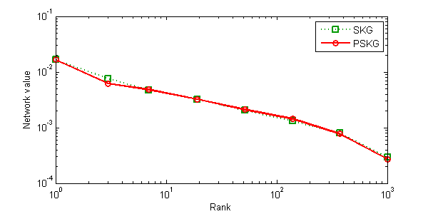
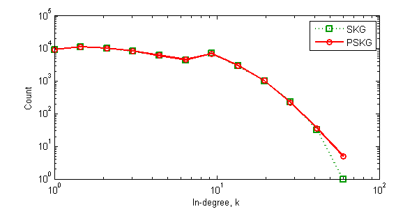
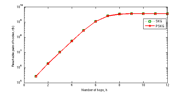
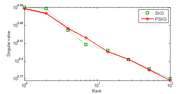
There are several standard graph patterns that are used to compare the similarity between networks. In this paper, we shall use the following patterns: degree distribution, hop plot, scree plot, and network values. These choices are motivated by Leskovec’s [7] work.

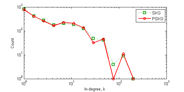
Degree distribution: The histogram of the nodes’ degrees with exponential binning.

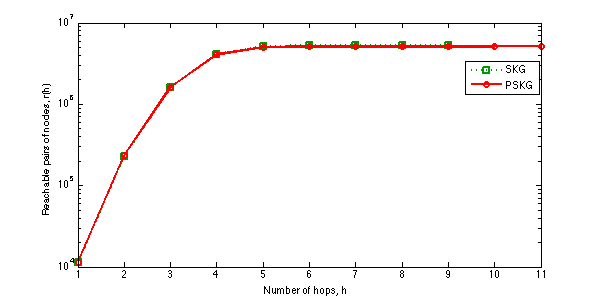
Hop plot: Number of reachable pairs $r(h)$ within $h$ hops, as a function of the number of hops $h$.

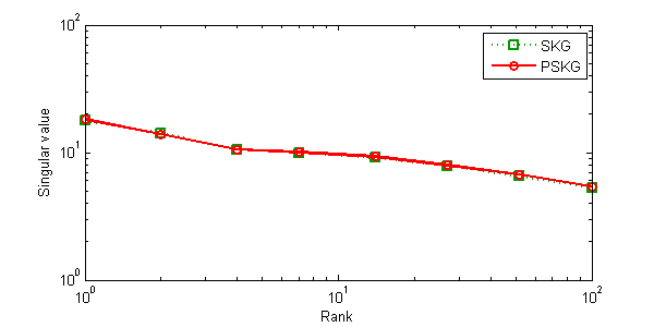
Scree plot: Singular values of the graph adjacency matrix versus their rank.

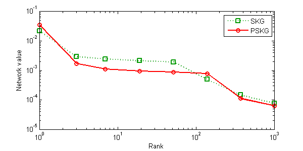
Network values: Distribution of the principal eigenvector components versus their rank.

Figure 3 and Figure 4 compares the graph patterns of SKG and PSKG. It is clear that the results are essentially the same.

(a) Degree distribution

(b) Hop plot

(c) Scree plot

(d) “Network value”

Figure 3: Graph patterns with parameters $n=2$, $k=12$, $E=11400$, and $P=[0.4532,0.2622;0.2622,0.0225]$

(a) Degree distribution

(b) Hop plot

(c) Scree plot

(d) “Network value”

Figure 4: Graph patterns with parameters $n=4$, $k=8$, $E=263546$, and $P=[\alpha,\alpha,\alpha,\alpha;\alpha,\alpha,\beta,\beta;\alpha,\beta,\alpha,\beta;\alpha,\beta,\beta,\alpha]$ where $\alpha=0.0861$ and $\beta=0.0231$. $P$ is the adjacency matrix of a star graph on 4 nodes (center + 3 satellites) with the $1$’s are replaced with $\alpha$ and the $0$’s are replaced with $\beta$.

4 Conclusion

In conclusion, PSKG is a network generation model that is more efficient than and yet as powerful as SKG. Section 2 and 3 each provide theoretical and empirical evidence to this statement.

One promising direction of future work is vertex-centric algorithms for model estimation. There has been much work on SKG model fitting, which should directly apply to PSKG, but most do not concern vertex-centric parallelism. It would be interesting to see the efficiency a vertex-centric distributed fitting algorithm can achieve compared to a serial or MapReduce implementation.

References

- [1] Milton Abramowitz and Irene A. Stegun “Handbook of Mathematical Functions with Formulas, Graphs, and Mathematical Tables” New York: Dover Publications, 1964
- [2] “Apache Giraph” URL: http://giraph.apache.org/
- [3] “Apache Hama” URL: http://hama.apache.org/
- [4] Morton B. Brown and Judith Bromberg “An Efficient Two-Stage Procedure for Generating Random Variates from the Multinomial Distribution” In The American Statistician 38.3 American Statistical Association, 1984, pp. pp. 216–219
- [5] Deepayan Chakrabarti, Yiping Zhan and Christos Faloutsos “R-MAT: A recursive model for graph mining” In In SDM, 2004
- [6] “Giraph Patch on Creating Randomized Synthetic Graph” URL: https://issues.apache.org/jira/browse/GIRAPH-26
- [7] Jure Leskovec et al. “Kronecker Graphs: An Approach to Modeling Networks” In J. Mach. Learn. Res. 11 JMLR.org, 2010, pp. 985–1042
- [8] Grzegorz Malewicz et al. “Pregel: a system for large-scale graph processing” In Proceedings of the 2010 ACM SIGMOD International Conference on Management of data, SIGMOD ’10 Indianapolis, Indiana, USA: ACM, 2010, pp. 135–146 DOI: 10.1145/1807167.1807184
- [9] Semih Salihoglu and Jennifer Widom “GPS: A Graph Processing System” Stanford InfoLab
- [10] “SNAP Network Analysis Library” URL: http://snap.stanford.edu/