Massless Dirac particle in a stochastic magnetic field: A solvable quantum walk approximation

A massless Dirac particle is considered, moving along the $x$-axis while Pauli-coupled by its anomalous magnetic moment to a piecewise constant magnetic field along the same axis, with stochastically varying sign. The motion is approximated as a quantum walk with unitary noise, for which the evolution can be found exactly. Initially ballistic, the motion approaches a classical diffusion on a time-scale determined by the speed of light, the size of the magnetic moment, the strength of the field and the time interval between changes in its direction. It is suggested that a process of this type could occur in the Sun’s corona, significantly affecting the solar fluxes of one or more neutrino types.

1 Introduction

It is known that the time-evolution of some free-particle relativistic wave equations can be approximated by a quantum walk (QW). This connection has its origins in Feynman’s path-integral approach to the propagator for Dirac’s equation [1, 2], and so predates the extensive researches into QWs and their potential for applications in quantum information theory that have followed from the seminal paper of Aharonov et al. [3].

The connection has been explored in work by Childs and Goldstone on the massless Dirac equation [4], by Katori et al. [5] on Weyl’s neutrino equation, and by Strauch [6] and us [7] on Dirac’s equation with a non-zero mass. As a result it is now well-understood how the dynamics of a free relativistic particle with spin $1/2$ , moving on a line, can be approximated arbitrarily closely by a simple, one-dimensional QW.

Because the free Weyl and Dirac equations can be solved easily and exactly, the connections with QWs are mathematically interesting but of limited importance to relativistic physics. In contrast, we consider here a relativistic quantum system that does not seem to be amenable to analysis unless approximated as a noisy QW.

Hackett [8] considered the effect of adding an arbitrarily small amount of classical randomness in a unitary way to a simple QW on the line. The idea of a QW contaminated by unitary noise was then explored extensively by Shapira et al. [9]. An initially ballistic motion with a spreading rate proportional to the elapsed time, as typical of a QW, is eventually replaced by a diffusive motion, with a spreading rate proportional to the square-root of the time, as typical of a classical random walk (CRW). The transition occurs after a time (number of iterations) determined by the strength of the noise. Addition of noise in other forms to QWs has been shown to produce similar effects [10, 11].

Recently we have studied a particularly simple one-dimensional QW with unitary noise, with the property that an initially diagonal density matrix remains diagonal during the evolution of the system [12, 13]. The form of this evolving density matrix has been found exactly. This simple system may be regarded as a toy model for QWs with unitary noise, and it does exhibit the transition from ballistic to diffusional behavior explicitly.

What we now show is that, despite its simplicity, this model has an application to the description of a neutral, massless Dirac particle with anomalous magnetic moment, Pauli-coupled to a piece-wise constant magnetic field with stochastically changing direction, and confined to move on a straight line.

The interpretation of the transitional behavior of the QW in the context of this relativistic system is rather remarkable: at short times $t$ there is a high probability of finding the particle at a distance $ct$ from its starting point, where $c$ is the speed of light, as expected for a free massless particle. But as time passes, the motion tends more and more towards a diffusion on the line, with a high probability of finding the particle within a distance $\alpha\sqrt{t}$ of a certain point $x_{0}$ as a normal distribution is approached, centered on that point. Here $\alpha$ is a constant whose value, together with that of $x_{0}$, is determined by the speed of light, the magnetic moment, the strength of the magnetic field, and the time interval between changes in field direction.

2 The relativistic system

The dynamics of the particle in this case is governed by Dirac’s equation in the form

$$i\hbar\,\partial\,\psi({\vec{x}},t)/\partial\,t=H(t)\psi({\vec{x}},t)\,,\quad$$

$${\rm where}\quad H(t)=c{\vec{\alpha}}\cdot{\vec{p}}-\mu\,\beta\,{\vec{S}}\cdot{\vec{B}}(t)\,.$$ (1)

Here ${\vec{p}}=-i\hbar\partial/\partial{\vec{x}}$ is the momentum $3$-vector, $\mu$ is the magnetic moment, ${\vec{B}}(t)$ is the external magnetic field $3$-vector, and ${\vec{S}}$ is the spin $3$-vector. The $4\times 4$ matrices in (1) are conveniently defined in terms of the $2\times 2$ Pauli matrices ${\vec{\sigma}}$ and $2\times 2$ unit matrix $I_{2}$ by

$${\vec{\alpha}}=\sigma_{3}\otimes{\vec{\sigma}}\,,\quad\beta=\sigma_{2}\otimes I_{2}\,,\quad{\vec{S}}={\textstyle\frac{1}{2}}\,\hbar\,I_{2}\otimes{\vec{\sigma}}\,.$$ (2)

Can such a system be realized in Nature or the laboratory? We postpone a discussion of this until the end of the paper; at this stage our objective is to add to the collection of relativistic systems amenable to mathematical analysis.

To proceed, suppose that $p_{\,2}\,|\psi\rangle=p_{\,3}\,|\psi\rangle=0$ on states $|\psi(t)\rangle=\psi(x,t)$ of interest, writing $x_{1}=x$, $p_{1}=p=-i\hbar\partial/\partial x$. We consider magnetic fields of the form ${\vec{B}}(t)=(B(t),\,0,\,0)$ with

$$B(t)=sB_{0}\,,\quad N\Delta<t<(N+1)\Delta\,,\quad N=0,\,1,\,\dots\,,$$ (3)

where $\Delta>0$ and $B_{0}$ are constants, and $s=\pm 1$, each sign having probability $1/2$, independently at each value of $N$. Under these assumptions, the helicity operator ${\textstyle\frac{1}{2}}I_{2}\otimes\sigma_{1}$ is a constant of motion, and we may suppose for definiteness that

$$(I_{2}\otimes\sigma_{1})|\psi\rangle=|\psi\rangle\,,$$ (4)

and work henceforth in this eigenspace, neglecting the action of the Pauli matrices in the second factor of the tensor product. Now the Hamiltonian reduces effectively to

$$H=cp\,\sigma_{3}-(\hbar\mu B(t)/2)\,\sigma_{2}\,,$$ (5)

and the evolution operator carrying $|\psi(t=n\Delta)\rangle$ into $|\psi(t=(n+1)\Delta)\rangle$ reduces to

$$V(s) = \exp\{-i[cp\sigma_{3}-s(\hbar\mu B_{0}/2)\,\sigma_{2}]\Delta/\hbar\}\,.$$ (6)

3 Approximation as a noisy quantum walk

The key step in our approximate treatment is to write from (6)

$$V(s) \approx \exp\{-i[cp\Delta/\hbar]\sigma_{3}\}\,\,\exp\{i[s\mu B_{0}\Delta/2]\sigma_{2}\}\,.$$ (7)

Bearing in mind the Campbell-Baker-Hausdorff formula [14], we assume that (7) is a good approximation provided

$$|c\langle p\rangle_{n}\Delta/\hbar|\ll 1\quad{\rm and}\quad|\mu B_{0}\Delta/2|\ll 1\,,$$ (8)

where $\langle p\rangle_{n}$ is the expectation value of $p$ in the state $|\psi(t=n\Delta)\rangle$. We shall not attempt here a more rigorous analysis of the approximation (7), analogous to that given for the free-particle [7], but content ourselves with the assumption that inequalities (8) hold so strongly for each $n=0\,,1\,,2\,,\dots\,,N$ that there is a negligible accumulation of errors when the approximate evolution operators in the form (7) are applied $N$ times to $|\psi(0)\rangle$, while the system evolves over a time $t=N\Delta$ of interest (see below).

The operators (5), (6) and (7) act on the Hilbert space ${\cal H}={\cal H}_{W}\otimes{\cal H}_{C}$, where ${\cal H}_{W}$ is the space of square-integrable functions of $x$ on which $p$ acts, and ${\cal H}_{C}$ is the 2-dimensional complex vector space on which the Pauli matrices in (5) and (6) act, each space having the usual scalar product. In ${\cal H}_{W}$ we introduce the infinite sequence of orthonormal states $|k\rangle$ defined by

$$|k\rangle=F(x-kc\Delta)\,,\quad k=0\,,\pm 1\,,\pm 2\,,\dots\,,$$ (9)

where $F(x)$ is some chosen smooth function with compact support ${\cal S}<(-c\Delta/2,c\Delta/2)$, satisfying

$$\int_{\cal S}|F(x)|^{2}\,dx=1\,.$$ (10)

Note that the states $|k\rangle$ do not in general form a basis in ${\cal H}_{W}$. We also introduce on ${\cal H}_{W}$, the translation operators

$$E_{\pm}=\exp{(\mp icp\Delta/\hbar)}\,,\quad E_{\pm}|k\rangle=|k\pm 1\rangle\,.$$ (11)

In ${\cal H}_{C}$ we introduce the orthonormal basis of states $|\tau\rangle$, $\tau=\pm 1$, with

$$\sigma_{3}|\pm 1\rangle=\pm|\pm 1\rangle\,,$$ (12)

and the associated orthogonal projection operators

$$P_{\pm}={\textstyle\frac{1}{2}}(I_{2}\pm\sigma_{3})\,,\quad P_{\pm}|\pm 1\rangle=|\pm 1\rangle\,,\quad P_{\pm}|\mp 1\rangle=0\,.$$ (13)

Now we can rewrite (7) as

$$V(s)=E_{+}\otimes P_{+}U(s)+E_{-}\otimes P_{-}U(s)\,,$$ (14)

where

$$U(s) = \exp\{i[s\mu B_{0}\Delta/2]\sigma_{2}\}$$ (15)

$$= \cos(\mu B_{0}\Delta/2)I_{2}+is\sin(\mu B_{0}\Delta/2)\sigma_{2}\,.$$

In (14) we have introduced $\otimes$ to separate explicitly the spatial and spin degrees of freedom. Adopting the standard matrix form for $\sigma_{2}$, we have from (15) the matrix representation

$$U(s)={\cal N}\left[\begin{array}[]{l}1\quad\quad\quad s\epsilon\\ -s\epsilon\quad\quad 1\end{array}\right]\,,$$ (18)

where

$$\epsilon=\tan(\mu B_{0}\Delta/2)\,,\quad{\cal N}=1/\sqrt{1+\epsilon^{2}}\,.$$ (19)

Here we have used $\cos(\mu B_{0}\Delta/2)\geq 0$, which follows from the second of conditions (8).

At this point we recognize (14) as the evolution operator for a QW on a line with unitary noise [8, 9, 12, 13]. In that context, ${\cal H}_{W}$ is the ‘walker’ space and ${\cal H}_{C}$ the ‘coin’ space, $E_{\pm}$ governs steps by the walker to right or left on the line, and $U(s)$ is the ‘reshuffling matrix’. The walk is an essentially trivial one, with $U=I_{2}$, contaminated by unitary noise that is characterized by the parameter $\epsilon$ and the random variable $s$.

4 Analysis

Depending on the direction of the magnetic field, the initial state vector $|\psi(0)\rangle$ evolves to either

$$|\psi(\Delta)\rangle=V(+1)\,|\psi(0)\rangle\quad{\rm or}\quad|\psi(\Delta)\rangle=V(-1)\,|\psi(0)\rangle\,,$$ (20)

at time $t=\Delta$, each possibility occurring with probability $1/2$. But this simply means that the initial density operator $\rho(0)=|\psi(0)\rangle\langle\psi(0)|=\rho_{0}$, say, evolves into

$$\rho(\Delta)=\rho_{1}={\textstyle\frac{1}{2}}\sum_{s=\pm 1}V(s)\rho_{0}V(s)^{\dagger}\,.$$ (21)

More generally, at time $t=N\Delta$, the density operator is

$$\rho(N\Delta)=\rho_{N}\qquad\qquad\qquad\qquad\qquad\qquad\qquad\qquad\qquad\qquad\qquad\qquad$$

$$=\frac{1}{2^{N}}\sum_{s_{1},s_{2},\,\dots\,,s_{N}}V(s_{N})\dots V(s_{2})V(s_{1})\,\rho_{0}\,V(s_{1})^{\dagger}V(s_{2})^{\dagger}\dots V(s_{N})^{\dagger}\,,$$ (22)

each $s_{n}$ being summed over the values $\pm 1$.

Consider the case with

$$|\psi(0)\rangle=|k=0\rangle\otimes|\tau=+1\rangle\,,$$ (23)

so that

$$\rho_{0}=|0\rangle\langle 0|\otimes\left[\begin{array}[]{l}1\quad\quad 0\\ 0\quad\quad 0\end{array}\right]\,,$$ (26)

using again the matrix representation as in (18). We postpone to the end of the paper a discussion of the difficulty of finding a positive energy state in this form for the system with Hamiltonian (5). In this case,

$$V(+1)|\psi(0)\rangle = {\cal N}\left(E_{+}\otimes\left[\begin{array}[]{l}1\quad\quad\epsilon\\ 0\quad\quad 0\end{array}\right]+E_{-}\otimes\left[\begin{array}[]{l}0\quad\quad 0\\ -\epsilon\quad\quad 1\end{array}\right]\right)$$ (31)

$$\qquad\qquad\times\left(|0\rangle\otimes\left[\begin{array}[]{l}1\\ 0\end{array}\right]\right)$$ (34)

$$= {\cal N}\left(|1\rangle\otimes\left[\begin{array}[]{l}1\\ 0\end{array}\right]+|-1\rangle\otimes\left[\begin{array}[]{l}0\\ -\epsilon\end{array}\right]\right)\,.$$ (39)

It follows that

$$V(+1)\,\rho_{0}\,V(+1)^{\dagger}={\cal N}^{2}\left(|1\rangle\langle 1|\otimes\left[\begin{array}[]{l}1\quad\quad 0\\ 0\quad\quad 0\end{array}\right]\right.$$ (42)

$$\left.+|1\rangle\langle-1|\otimes\left[\begin{array}[]{l}0\quad\quad-\epsilon\\ 0\quad\quad 0\end{array}\right]+|-1\rangle\langle 1|\otimes\left[\begin{array}[]{l}0\quad\quad 0\\ -\epsilon\quad\quad 0\end{array}\right]\right.$$ (47)

$$\left.+|-1\rangle\langle-1|\otimes\left[\begin{array}[]{l}0\quad\quad 0\\ 0\quad\quad\epsilon^{2}\end{array}\right]\right)\,.$$ (50)

The expression for $V(-1)\,\rho_{0}\,V(-1)^{\dagger}$ is similar, with $\epsilon$ replaced by $-\epsilon$ throughout, and it then follows from (21) that in this case

$$\rho_{1}={\cal N}(\epsilon)^{2}\left(|1\rangle\langle 1|\otimes\left[\begin{array}[]{l}1\quad\quad 0\\ 0\quad\quad 0\end{array}\right]\right.$$ (53)

$$\left.+|-1\rangle\langle-1|\otimes\left[\begin{array}[]{l}0\quad\quad 0\\ 0\quad\quad\epsilon^{2}\end{array}\right]\right)\,.$$ (56)

We see that $\rho_{1}$, like $\rho_{0}$, is diagonal in the space of states spanned by all the vectors $|k\rangle\otimes|\tau\rangle$. It is easily shown by induction that the same is true of $\rho_{N}$ for each non-negative integer $N$, and that in fact $\rho_{N}$ has the form

$$\rho_{N}=\sum_{k=-N}^{N}\,\!{}^{{}^{\prime}}|k\rangle\langle k|\otimes\left[\begin{array}[]{l}\alpha_{N\,k}\quad\quad 0\\ 0\quad\quad\beta_{N\,k}\end{array}\right]\,,$$ (59)

where the prime indicates that the sum is over the $N+1$ values $-N\,,-N+2\,,\dots\,,N$ of $k$, and the constants $\alpha_{N\,k}$, $\beta_{N\,k}$ are non-negative.

It is also easily shown [12, 13] from (22) that $\alpha_{N\,k}$, $\beta_{N\,k}$ are determined by the coupled recurrence relations

$$\alpha_{N+1\,k}={\cal N}^{2}\,(\alpha_{N\,k-1}+\epsilon^{2}\beta_{N\,k-1})\,,\quad\!\!\!k=-N+1\,,-N+3\,,\dots\,,N+1\,,$$

$$\beta_{N+1\,k}={\cal N}^{2}\,(\beta_{N\,k+1}+\epsilon^{2}\alpha_{N\,k+1})\,,\quad\!\!\!k=-N-1\,,-N+1\,,\dots\,,N-1\,,$$

$${\rm for}\quad N=0\,,1\,,2\,,\dots\,,\qquad\qquad\qquad$$ (60)

with the initial conditions

$$\alpha_{0\,0}=1\,,\qquad\beta_{0\,0}=0\,,\quad\alpha_{0k}=\beta_{0k}=0\,,\quad k\neq 0\,.$$ (61)

For example, (56) shows that

$$\alpha_{1\,1}={\cal N}^{2}\,,\quad\alpha_{1\,-1}=0\,,\quad\beta_{1\,1}=0\,,\quad\beta_{1\,-1}={\cal N}^{2}\,\epsilon^{2}\,.$$ (62)

Note that

$$\langle+1|\otimes\langle k|\,\rho_{N}\,|k\rangle\otimes|+1\rangle=\alpha_{Nk}\,,\quad\langle-1|\otimes\langle k|\,\rho_{N}\,|k\rangle\otimes|-1\rangle=\beta_{Nk}\,,$$ (63)

so that $\alpha_{Nk}$ (resp. $\beta_{Nk}$) is the probability of finding the particle in the state $|k\rangle\otimes|+1\rangle$ (resp. $|k\rangle\otimes|-1\rangle$) on measurement. Then

$$P_{Nk}=\alpha_{Nk}+\beta_{Nk}$$ (64)

is the probability that the particle will be found in the state $|k\rangle$, with the value of $\tau$ immaterial. Because the state $|k\rangle$ can be localized as closely as we like about $x=kc\Delta$, we may say that $P_{Nk}$ is the probability of finding the particle ‘at’ that place, at time $t=N\Delta$.

When $\epsilon=0$, the solution of (60) and (61) is $\alpha_{NN}=1$, with all other $\alpha_{Nk}$ and all $\beta_{Nk}$ vanishing. The massless particle is free, and marches to the right at speed $c$, with probability $P_{NN}=1$ of being at $x=Nc\Delta=ct$ at time $t=N\Delta$. If we had chosen $\tau=-1$ in the initial state, the particle would have marched to the left. In each case the motion is always purely ballistic; there is no transition to diffusional evolution at large times, because there is no noise contaminating the QW, which has the trivial reshuffling matrix $U=I_{2}$. If we were to choose an initial mixed state instead of (26), taking $\rho_{0}=|0\rangle\langle 0|\otimes I_{2}/2$, the resulting probability distribution on the $x$-axis would have $P_{NN}=P_{N\,-N}=1/2$, giving an extreme example of the familiar two-horned distributions associated with simple QWs on the line [15].

When $\epsilon=1$, (60) and (64) show that

$$P_{N+1\,k}={\textstyle\frac{1}{2}}(P_{N\,k-1}+P_{N\,k+1})\,,$$ (65)

which is the defining rule for the Pascal’s triangle of successive probability distributions centered on $k=0$ for a simple classical random walk (CRW), leading to

$$P_{Nk}=\frac{1}{2^{N}}\,C^{N}_{(N+k)/2}\,,\quad k=-N\,,-N+2\,,\dots\,,N$$ (66)

for $N=0\,,1\,,2\,,\dots$, where $C^{p}_{q}=p!/q!(p-q)!$ is the binomial coefficient. Then (60) and (61) give

$$\alpha_{Nk}={\textstyle\frac{1}{2}}P_{N-1\,k-1}=\frac{1}{2^{N}}\,C^{N-1}_{(N+k-2)/2}\,,\quad k=-N+2\,,-N+4\,,\dots N\,,$$

$$\beta_{Nk}={\textstyle\frac{1}{2}}P_{N-1\,k+1}=\frac{1}{2^{N}}\,C^{N-1}_{(N+k+2)/2}\,,\quad k=-N\,,-N+2\,,\dots N-2\,,$$

$$\alpha_{N\,-N}=0\,,\quad\beta_{N\,N}=0\,,\quad\alpha_{0\,0}=1\,,\quad\beta_{0\,0}=0\,.\qquad\qquad$$ (67)

Thus there is no ballistic regime in this case; the evolution is purely diffusional. As is well known [16], the distribution (66) is asymptotic to a continuous, normal one centered on $k=0$ as $N\to\infty$, with density

$$P(N,k)=\frac{e^{-k^{2}/2N}}{\sqrt{2N\pi}}\,,\qquad-\infty<k<\infty\,.$$ (68)

Then we can say that after a time $t=N\Delta$ with $N\gg 1$, there is $95\%$ probability that the particle can be found within two standard deviations of the origin, that is to say, with $|x|<2\sqrt{N}c\Delta=2c\sqrt{t\Delta}$, in sharp contrast to the behavior of the free, massless particle, which would always be found at a distance $ct$ from the origin.

In terms of the physical variables of the relativistic particle, we have asymptotically as $t=N\Delta\to\infty$, the density

$${\cal P}(t,x)=\frac{e^{-x^{2}/4Dt}}{\sqrt{4\pi Dt}}\,,\qquad-\infty<x<\infty\,,\quad D=c^{2}\Delta/2\,.$$ (69)

Note however that (8) requires $\epsilon\ll 1$, so that our approximate treatment of the relativistic system may break down when $\epsilon=1$.

For general values of $\epsilon$, the solution of (60) and (61) has been found in the form [13]

$$\alpha_{NN}=Q(N,N)\,,\quad\beta_{NN}=0\,,\qquad\qquad\qquad\qquad$$

$${\rm and}\qquad\qquad\qquad\qquad\qquad\qquad\qquad\qquad\qquad\qquad\qquad\qquad\qquad\qquad$$

$$\alpha_{N\,k}=Q(N,k)-Q(N-1,k+1)/(1+\epsilon^{2})\,,\qquad\qquad$$

$$\beta_{N\,k}=\epsilon^{2}Q(N-1,k+1)/(1+\epsilon^{2})\,,\qquad\qquad\qquad$$ (70)

for $k=-N\,,-N+2\,,\dots\,,N-2$, where

$$Q(N,k)=\frac{1}{(1+\epsilon^{2})^{N}}\,\sum_{s=0}^{(N-|k|)/2}\,C^{N-2s}_{(N-k-2s)/2}\,C^{N-s}_{s}\,(\epsilon^{4}-1)^{s}\,.$$ (71)

Then (64) gives

$$P_{NN}=Q(N,N)\,,\quad{\rm and}\quad P_{N\,k}=Q(N,k)-\frac{1-\epsilon^{2}}{1+\epsilon^{2}}\,Q(N-1,k+1)$$

$${\rm for}\quad k=-N\,,-N+2\,,\dots\,,N-2\,.\qquad\qquad\qquad$$ (72)

As $N=t/\Delta$ increases for any given $0<\epsilon<1$, the probability distribution (72) undergoes the transition from ballistic evolution to diffusive evolution mentioned in the Introduction. This is seen in Fig. 1, which shows probability versus $x/c\Delta=k$ in the case $\epsilon=0.2$, for $N=t/\Delta=20\,,50\,,100\,,200\,.$ The plots reveal also that during the transition, the probability distribution may be considered to consist of two components: (1) the probability at the point $x=ct$ corresponding to ballistic motion of the massless particle at speed $c$, marked by the circled point on the right in each plot, which decreases as time $t=N\Delta$ increases, and (2) a growing diffusional distribution on $x$-values closer to the origin, eventually swamping the ballistic component, and approaching a normal distribution centered on a mean positive displacement.

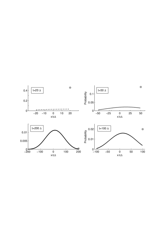
Figure 1: Clockwise from Top Left: Plots of probability against $x/c\Delta$, for $t=20\Delta\,,50\Delta\,,100\Delta\,,200\Delta$, with $\epsilon=0.2$. The probability at $x=ct$ is marked with a circled dot in each plot. Note the different scales on the axes in the plots.

This transition is reflected in the behavior of $P_{NN}$, the probability that the particle is at $x=ct$ at time $t=N\Delta$ (the circled dot on the plots in Fig. 1). This probability equals $1$ in the free particle case $\epsilon=0$. From (72) and (71) we have in general

$$P_{NN}=[1/(1+\epsilon^{2})]^{N}\,C^{N}_{0}\,C^{N}_{0}=1/(1+\epsilon^{2})^{N}\,.$$ (73)

As $N=t/\Delta$ increases, there is a steady decline in the probability that the particle continues to travel at speed $c$ to the right. This is clear in the successive plots of Fig. 1, and is shown explicitly in Fig. 2.

Figure 2: Probability that the particle is at $x=ct$ after time $t$, in the case $\epsilon=0.2$.

It is also instructive to consider the moments of the probability distribution (72), defined for each $N$ as

$$S_{N}^{(p)}=\sum_{k=-N}^{N}\,\!{}^{\prime}\,P_{Nk}\,k^{p}\,,\quad p=0\,,1\,,2\,,\dots\,.$$ (74)

The zeroth, first and second moments have been calculated exactly [13], as

$$S_{N}^{(0)}=1\,,\quad S_{N}^{(1)}=\frac{(1-\epsilon^{2})}{2\epsilon^{2}}\,\left[1-\left(\frac{1-\epsilon^{2}}{1+\epsilon^{2}}\right)^{N}\right]\,,$$

$$S_{N}^{(2)}=\frac{1}{2\epsilon^{4}}\left[2N\epsilon^{2}-1+\epsilon^{4}+\frac{(1-\epsilon^{2})^{N+1}}{(1+\epsilon^{2})^{N-1}}\right]\,.$$ (75)

In the ballistic regime, $N\epsilon^{2}\ll 1$, and

$$(1-\epsilon^{2})^{N+1}/(1+\epsilon^{2})^{N-1}=1-\epsilon^{4}-2N\epsilon^{2}+2N^{2}\epsilon^{4}+{\rm O}([N\epsilon^{2}]^{3})\,,$$ (76)

so that

$$S_{N}^{(2)}=\frac{1}{\epsilon^{4}}(N\epsilon^{2})^{2}+{\rm O}([N\epsilon^{2}]^{3})\,.$$ (77)

The rate of growth of the second moment, quadratic in $N$, is characteristic of a QW [15].

In the diffusive regime, $N\epsilon^{2}\gg 1$, and

$$S_{N}^{(2)}=\frac{1}{\epsilon^{4}}\,(N\epsilon^{2})-\frac{1-\epsilon^{4}}{2\epsilon^{4}}+{\rm O}(1/[N\epsilon^{2}])\,,$$ (78)

showing the rate of growth is now linear in $N$, as typical of a CRW [16]. Note that however small is $\epsilon^{2}$, eventually $N$ becomes so large that the second regime is reached. The changeover occurs in the region where $N\epsilon^{2}={\rm O}(1)$. This is the behavior observed in numerical simulations of quantum walks with unitary noise [9], of which the present process may be considered a simple, special case, with the advantage that it is more amenable to mathematical analysis.

Note also that the second moment can be interpreted as the expectation value $\langle(x/c\Delta)^{2}\rangle$. Fig. 3 shows the transition from quadratic to linear behavior of this quantity with increasing $N=t/\Delta$ in the case $\epsilon=0.2$.

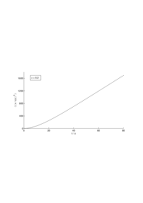
Figure 3: Change from quadratic to linear growth of $\langle(x/c\Delta)^{2}\rangle$ with increasing $t=N\Delta$, in the case $\epsilon=0.2$. The transition occurs in the neighborhood of $N=25$, where $N\epsilon^{2}=1$.

The asymptotic behavior as $N\to\infty$ of the moments of the distribution (72), defined as in (74), has also been calculated [13], to give

$$S_{N}^{(2n)}\sim\frac{N^{n}\,(2n-1)!}{(n-1)!\,2^{n-1}\epsilon^{2n}}\,,\qquad\qquad$$

$$S_{N}^{(2n+1)}\sim\frac{N^{n}\,(2n+1)!}{n!\,2^{n}\epsilon^{2n}}\frac{1-\epsilon^{2}}{2\epsilon^{2}}\,,$$ (79)

for $n=0\,,1\,,2\,,\dots$. From this it follows that as $N\to\infty$, the probability distribution given by $P_{Nk}$ is asymptotic to a continuous, normal distribution with density

$$P(N,k)=\frac{e^{-\epsilon^{2}\,(k-k_{\,0})^{2}/2N}}{\sqrt{2N\pi/\epsilon^{2}}}\,,\qquad-\infty<k<\infty\,,$$ (80)

where $k_{0}=(1-\epsilon^{2})/2\epsilon^{2}$. This generalizes the result (68), which is recovered when $\epsilon=1$. Fig. 4 shows the degree of agreement between the exact and asymptotic probability densities for $\epsilon=0.2$ with $N=t/\Delta=100$ and $N=300$; in the latter case, the plots sit almost one on top of the other. Note that because the $P_{Nk}$ are defined at $k$-values two units apart, we have for each value of $N$,

$$\sum_{k=-\infty}^{\infty}\,{\textstyle\frac{1}{2}}P_{Nk}\,\Delta_{k}=1\,,\quad\Delta_{k}=2\,,$$ (81)

showing that it is the set of values ${\textstyle\frac{1}{2}}P_{Nk}$, $k=-N\,,-N+2\,,\dots\,,N$ that is to be considered a probability density for comparisons as in Fig. 4 with the continuous density $P(N,k)$.

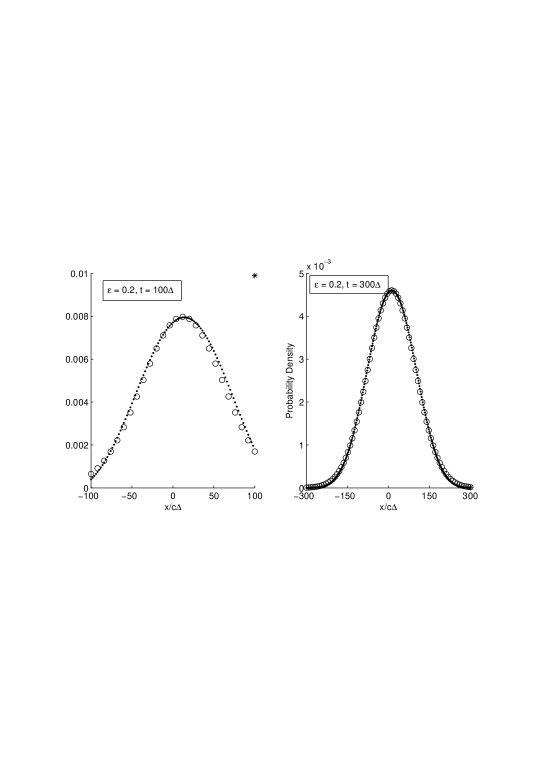
Figure 4: Comparison of the discrete probability density ${\textstyle\frac{1}{2}}P_{Nk}$, $k=-N\,,-N+2\,,\dots\,,N$, marked with dots, with the asymptotic normal form $P(N,k)$, marked with circles, for $\epsilon=0.2$ and $N=100\,,300$. Note the value at $x=ct$ marked with an asterisk in the first plot.

For a general value of $\epsilon$, we now have that as $t=N\Delta\to\infty$, the probability density on the $x$-axis is asymptotic to that for the normal distribution

$${\cal P}(t,x)=\frac{e^{-(x-x_{\,0})^{2}/(4Dt)}}{\sqrt{4\pi Dt}}\,,\qquad-\infty<x<\infty\,,$$

$$x_{0}=(1-\epsilon^{2})c\Delta/2\epsilon^{2}\,,\quad D=c^{2}\Delta/2\epsilon^{2}\,.$$ (82)

Here the displacement of the mean position $\langle x\rangle$ of the particle at large times, to the value $x_{0}$, is noteworthy. Using (19), we see that this value is given in terms of the physical variables defining the Hamiltonian as

$$x_{0}=\frac{\cos(\mu B_{0}\Delta)}{1-\cos(\mu B_{0}\Delta)}\,c\Delta\,.$$ (83)

It can take any positive value, and is independent of the (very large value of the) time $t$. We can also say that as $t\to\infty$, there is a $95\%$ probability of finding the particle within two standard deviations of the mean; this is the probability to have $|x-x_{0}|<2c\sqrt{t\Delta}/\tan(\mu B_{0}\Delta/2)$.

5 Discussion

The transition from ballistic to diffusional behavior in QWs with unitary noise is surprising; in the context of a relativistic quantum system as we have discussed here, it is even more remarkable. Diffusion commonly arises as a non-relativistic, classical process. Note from (19) and (82) the dependence of the associated diffusion coefficient $D$ on the speed of light as well as on the magnetic moment, the strength of the magnetic field, and the time interval between changes in field direction.

Can a system of the type we have described be realized physically? There are several difficulties standing in the way. In the first place, it is now thought that all neutrinos have small rest masses, leaving us with no candidate massless Dirac particles. Even if it should transpire that one of the neutrino types is after all massless, there is no evidence for neutrino magnetic moments, although there has long been speculation that such might exist [17, 18, 19, 20, 21].

Could the model apply to neutrinos, or indeed to the neutron, in situations where the rest-mass contribution $mc^{2}\beta$ now properly appearing as an extra term in the Hamiltonian (1), can nevertheless be neglected relative to the magnetic interaction term, so that (1) still applies? Evidently, this would require

$$|\hbar\mu B_{0}/2|\gg mc^{2}$$ (84)

in addition to the conditions (8). Inserting the observed values of $\mu$ and $m$ for the neutron gives values of $|B_{0}|$ several orders of magnitude greater than any that have been achieved in the laboratory, although it is conceivable that such field strengths could occur in extreme cosmological situations. Note that according to (8), extremely large $|B_{0}|$ values require extremely small field-oscillation times $\Delta$ if our approximate treatment is to be valid. In contrast to the situation for the free Dirac equation [7], where the size of $\Delta$ can be adjusted at will to ensure accuracy of the approximations used there, in the present case it is determined once the external magnetic field is prescribed.

For a neutrino (with anomalous magnetic moment) and very small rest mass, (84) is more easily satisfied. Although still unlikely in the laboratory, a process of the type we have described might apply in supernovas [22] or in the solar corona, for example, and affect significantly the fluxes of one or more neutrino types through the very strong stochastic magnetic fields occurring there [17, 18, 19, 23].

A more subtle difficulty that has been raised following (26) concerns the form of positive-energy states of the relativistic particle. Just as for a free electron [24], it is possible to construct positive-energy states of a free neutrino that are arbitrarily highly localized about any given point [25], and we could have used such a state in place of the $|\psi(0)\rangle$ in (23), supposing that the particle is free at $t=0_{-}$, and that the interaction is switched on at $t=0_{+}$. However, such a state and its translates do not have compact support and are not mutually orthogonal, severely complicating the analysis of the QW. Such a more complicated analysis is not warranted, in our opinion; for even if the particle is in a positive-energy state at $t=0_{-}$, it will not be so at $t=0_{+}$ when the field is switched on, because the Hamiltonian, and its positive energy states, change form. Similarly, even if it can be arranged that the particle is in a positive-energy state at $t=N\Delta_{-}$, it will not be so at $t=N\Delta_{+}$ if the field abruptly changes direction at that time, for the same reason. This difficulty, which is perhaps related to the Klein paradox [26], is not peculiar to the system we have discussed here, nor to our way of treating it. It seems clear that it must beset the analysis of a massless particle in any time-dependent, discontinuously changing external field. One could try to overcome the difficulty by projecting onto positive energy states immediately after each discontinuity occurs in the Hamiltonian, but it is not clear how to do this in a simple way that preserves the unitarity of the resulting time evolution and hence the length of the state vector.

We have not attempted to resolve this difficulty here, contenting ourselves with analyzing the model as described, in the belief that it makes an interesting addition to the collection of relativistic quantum systems that have been considered previously, and suggests that a quite new type of behavior can appear in such systems when subject to stochastically varying external fields. We hope that it provokes further study.

It would be interesting, and more realistic, to consider the Hamiltonian (1) for the neutron, with rest-mass term added, and evaluate the evolution numerically, without making any approximations like (7), to see if the stochastic nature of the interaction term continues to lead to diffusional behavior at large times. However, the second difficulty mentioned above would still require resolution.

The exact evolution in the massless case, associated with (6), could also be treated numerically to indicate any limitations of our approximate treatment.

Finally, it should be mentioned that the present model can also be considered in the context of quantum simulations of relativistic effects using the experimental apparatus of trapped ions. Indeed simulations of Dirac’s equation and associated relativistic quantum effects for a single trapped ion have already been proposed [27] and experimentally realized [28], especially concerning the simulation of the Zitterbewegung phenomenon and the Klein paradox [29, 30]. Simulations of a Dirac particle in a magnetic potential and its topological properties, using trapped ions, have also been proposed [31]. It is conceivable that the machinery of trapped ions might also allow a simulation of the Dirac QW driven by fluctuating magnetic fields that we have developed above, although it would be challenging for such simulations to overcome the physical obstacles indicated.

Acknowledgment: We thank the School of Mathematics and Physics, University of Queensland, for its hospitality during visits by D.E. (sabbatical) and I.S., when this work was completed.

References

- [1] R.P. Feynman and A.R. Hibbs, Quantum Mechanics and Path Integrals (McGraw-Hill, New York, 1965).
- [2] D.A. Meyer, J. Stat. Phys. 85, 551 (1996).
- [3] Y. Aharonov, L. Davidovich and N. Zagury, Phys. Rev. A 48, 1687 (1993).
- [4] A.M. Childs and J. Goldstone, Phys. Rev. A 70, 042312 (2004).
- [5] M. Katori, S. Fujino and N. Konno, Phys. Rev. A 72, 012316 (2005).
- [6] F.W. Strauch, Phys. Rev. A 73, 054302 (2006).
- [7] A.J. Bracken, D. Ellinas and I. Smyrnakis, Phys. Rev. A 75, 022322 (2007).
- [8] M. Hackett, Classical Randomness in a Quantum Walk on a Line (BSc Hons. thesis (unpublished), University of Queensland, 2001), www.maths.uq.edu.au/~ajb/.
- [9] D. Shapira, O. Biham, A.J. Bracken and M. Hackett, Phys. Rev. A 68, 062315 (2003).
- [10] T.A. Brun, H.A. Carteret and A. Ambainis, Phys. Rev. A 67, 032304 (2003).
- [11] V. Kendon and B. Tregenna, Phys. Rev. A 67, 042315 (2003).
- [12] D. Ellinas, A.J. Bracken and I. Smyrnakis, Discrete Randomness in Discrete Time Random Walk: Study via Stochastic Averaging, arXiv:1207.5257v1 [quant-ph] 22 Jul 2012, pp. 7, to appear in Reps. Math. Phys.
- [13] A.J. Bracken, D. Ellinas and I. Smyrnakis (in preparation).
- [14] W. Miller, Jr., Symmetry Groups and their Applications (Academic Press, New York, 1972).
- [15] A. Ambainis, E. Bach, A. Nayak, A. Vishwanath and J. Watrous, Proc. 33rd Annual ACM Symposium on Theory of Computing (STOC’01), 37 (2001).
- [16] B.D. Hughes, Random Walks and Random Environments, Vol. 1: Random Walks (Oxford University Press, New York, 1995).
- [17] A. Cisneros, Astrophys. Space Sc. 10, 87 (1971).
- [18] M.R. Voloshin, M.I. Vysotskii and L.B. Okun, Sov. Phys. JETP 64, 446 (1986).
- [19] E.Kh. Akhmedov and J. Pulido, Phys. Lett. B 553, 7 (2003).
- [20] A.O. Barut and A.J. Bracken, J. Math. Phys. 26, 1390 (1985).
- [21] H.T. Wong, Li H-B and Lin S-T, Phys. Rev. Letts. 105, 061801 (2010).
- [22] O.V. Lychkovskiy and S.I. Blinnikov, Phys. Atom. Nucl. 73, 614–624 (2010).
- [23] A.B. Balantekin and C. Volpe C, Phys. Rev. D 72, 033008 (2005).
- [24] A.J. Bracken, J. Flohr and G.F. Melloy, Proc. Roy. Soc. (London) A 461, 3633 (2005).
- [25] J.G. Wood, Asymptotic Localisation of Neutrinos in Relativistic Quantum Mechanics (BSc Hons. thesis (unpublished), University of Queensland, 1997), www.maths.uq.edu.au/~ajb/.
- [26] N. Dombey and A. Calogeracos, Phys. Rep. 315, 41 (1999).
- [27] L. Lamata L, J. León, T. Schätz and E. Solano, Phys. Rev. Lett. 98, 253005 (2007).
- [28] R. Gerritsma, G. Kirchmair, F. Zähringer, E. Solano, R. Blatt and C. F. Roos, Nature 463, 68 (2010).
- [29] J. Casanova, J. J. García-Ripoll, R. Gerritsma, C. F. Roos and E. Solano, Phys. Rev. A 82, 020101 (2010).
- [30] R. Gerritsma, B. P. Lanyon , G. Kirchmair, F. Zähringer, C. Hempel, J. Casanova, J. J. García-Ripoll, E. Solano, R. Blatt and C. F. Roos, Phys. Rev. Lett. 106, 060503 (2011).
- [31] L. Lamata, J. Casanova, R. Gerritsma, C. F. Roos, J. J. García-Ripoll and E. Solano, New J. Phys. 13, 095003 (2011) (cf. Ch. 4).