Electron-positron pair production in an arbitrary polarized ultrastrong laser field

Abstract

Electron-positron pair production in an arbitrary polarized ultrastrong laser field is investigated in the first order perturbation approximation in which the Volkov states are used for convenient calculation of scattering amplitude and cross section. It is found surprisingly that the optimal pair production depends strongly on the polarization. For some cases of field parameters, the optimal field is elliptically polarized or evenly circularly polarized one, rather than the usual linear polarization as indicated by previous works. Some insights into pair generation are given and some interesting unexpected features are also discussed briefly.

I Introduction

Strong field physics has been an active research field since the invention of the technique chirped pulse amplification (CPA) in 1985 StMo , which draws the intensity of tabletop laser from gigwatt to erawatt MoTaBu and makes it possible to test the quantum electrodynamics (QED) theory in laboratories Burke . The Stanford Linac Acceleration (SLAC) experiment in 1997 Burke ; Bamber have observed electrons-positrons ($e^{+}e^{-}$) pair production and revealed nonlinear QED effects, which have resurrected research interests in pair creation in strong fields. The forthcoming extreme-light-infrastructure (ELI) ELI will surely boost breakthrough in strong field physics research. This will be the strongest field in the world, though its intensity is approximately about $10^{25}\rm{W/cm^{2}}$ and still 4 orders less than the Schwinger’s critical field intensity $10^{29}\rm{W/cm^{2}}$ Schwinger .

Several methods in both of theory and numeric calculation have been proposed to analyze pair production in external fields since 1930s Sauter ; Volkov ; KimPa ; DuSc ; GiKl ; DuQHWGi ; MVG ; DeM ; MHaKe ; HuMKe ; Bulanov . One of the most important approaches is the perturbation method in which the corresponding Volkov states are used as bases. It was pioneered by Volkov Volkov , and developed by Reiss Reiss , Nikishov NiRi , Müller MVG ; DeM ; MHaKe ; HuMKe , Keitel MHaKe ; HuMKe and so on. But all of the above studies are based on particular polarized laser fields with either circular or linear polarization Reiss ; NiRi ; MVG ; DeM ; Bulanov ; MHaKe ; HuMKe . Most studies have manifested that the pair production rates are larger in linearly polarized fields compared than that in circular ones Altarelli ; DeM ; Popov ; Bulanov in some conditions. Albeit these progresses which have been achieved, no complete analytical or numerical studies have been performed to reveal the influence of laser fields with arbitrary polarization on pair creation, especially in the framework of perturbation method even though this method seems simple and valid for the problem. The reason may be that relatively tedious derivation of scattering amplitude and cross section is involved in that case of elliptic polarization where the scattering partial waves have many coupled terms.

Therefore, it is worthwhile to fill this research gap by exploring the relation between the elliptically polarized laser fields and pair production, which will give more insight into the SLAC experiment. Our study will show that a better pair production by elliptically polarized laser field can occur possibly. If we have got more information and recognition, it will be helpful not only to uncover more phenomena but also to regulate involved parameters in future experiments.

In the present paper, we will deal with one of these problems, through difficult theoretical and computing calculations. The case of head-on collision, occurring between a high-energy gamma photon and multiple photons of the laser fields, is considered. This process is called multi-photon reaction. Fortunately, we get the strict result in the framework of first order perturbation theory, and give thoroughly numerical calculations of some fixed parameters. There is, in fact, a surprising result that the pair creation relies strongly on the parameters of the laser fields, especially $\Upsilon$ (describing the elliptical polarization) in the condition that $\eta_{0}$ (the Lorentz-invariant dimensionless strength parameter GrRe ) could be compared with $\vartheta$ (the collision energy). The optimal filed is not the linearly polarized field, but in some cases it is elliptically polarized and sometimes even the circularly polarized.

The paper is organized as follows. Firstly, in Sec.II, we give a concrete theoretical derivation of the total cross section in the first order perturbation theory using the Volkov states wave functions. In Sec. III, we present some demonstrations of numerical results which show clearly and vividly how pair creation is influenced by a few important parameters such as the polarization $\Upsilon$, the Lorentz-invariant normalized field strength $\eta_{0}$, and the collision energy $\vartheta$. The main results will be summarized and some insights and discussions are given briefly in the final section.

II Theoretical formalism

In this section, we give a detailed derivation of the total pair production in the interaction between strong laser field and high energy photon. Some techniques used here are employed and developed from Ref. GrRe and Ref. BeLiPi . First of all, some notations must be employed for simplicity and convenience. Throughout the paper, an elliptically polarized laser field, $A^{\mu}=a[{\varepsilon}^{\mu}_{1}\cos{(k\cdot x)}+\Upsilon{\varepsilon}^{\mu}_{2}\sin{(k\cdot x)}]$, is adopted, where $a$ is the amplitude of vector potential $A$ of laser field, $k^{2}=0$, $k^{\mu}={\omega}(1,0,0,1)$, ${\varepsilon}^{\mu}_{1}=(0,1,0,0)$, ${\varepsilon}^{\mu}_{2}=(0,0,1,0)$ and $-1\leq\Upsilon\leq 1$. The natural units, $\hbar=c=1$, are also used.

We define $\Lambda=\frac{1}{2}(1+{\Upsilon}^{2})$, the average number density of photons ${\rho}(\omega)=\left\langle\frac{a^{2}\omega}{4\pi}[1+({\Upsilon}^{2}-1)\cos^{2}{(k\cdot x)}]\right\rangle=\frac{a^{2}\Lambda\omega}{4\pi}$ and $\eta=\frac{e}{m_{0}}\sqrt{\left|\left\langle A_{\mu}A^{\mu}\right\rangle\right|}=\frac{ea}{m_{0}}\sqrt{\Lambda}$, where $e$ and $m_{0}$ are respectively the charge and the rest mass of an electron. $\eta_{0}$ is defined as $\frac{ea}{m_{0}}$. The scalar four-product is defined as $A\cdot B=A_{\mu}B^{\mu}=A_{0}B^{0}-A_{i}B^{i}$ and $/\kern-6.99997ptA=A_{\mu}{\gamma}^{\mu}$, in which ${\gamma}^{\mu}$ is the standard Dirac matrices. We also sometimes use $\phi$ in place of $k\cdot x$ for brevity.

The solution of electrons/positrons under this type field could be well solved in terms of the known Volkov states Volkov ; GrRe , i.e. for electron it is $\Psi_{p,s}^{(e)}=N_{p}\left[1+\frac{e{/\kern-2.79996ptk}{/\kern-2.79996ptA}}{2(p\cdot k)}\right]u(p,s)\exp[iS^{(e)}_{(p,s)}(k\cdot x)]$ and for positron it is $\Psi_{\bar{p},-\bar{s}}^{(e^{+})}=N_{\bar{p}}\left[1-\frac{e{/\kern-2.79996ptk}{/\kern-2.79996ptA}}{2({\bar{p}}\cdot k)}\right]v(\bar{p},-\bar{s})\exp[iS^{(e^{+})}_{(\bar{p},-\bar{s})}(k\cdot x)]$. Here $u(p,s)$ and $v(\bar{p},-\bar{s})$ are respectively the unit spinor of a free electron and a free positron, $p$ and $\bar{p}$ the momenta, $s$ and $\bar{s}$ the spins, and $S^{(e)}_{(p,s)}$ and $S^{(e^{+})}_{(\bar{p},-\bar{s})}$ are

$$\left\{\begin{array}[]{l}S^{(e)}_{(p,s)}=-p\cdot x-\int\limits_{0}^{k\cdot x}\left[\frac{e(p\cdot A)}{p\cdot k}-\frac{e^{2}A^{2}}{2(p\cdot k)}\right]\,d\phi,\\ S^{(e^{+})}_{(\bar{p},-\bar{s})}=\bar{p}\cdot x-\int\limits_{0}^{k\cdot x}\left[\frac{e(\bar{p}\cdot A)}{\bar{p}\cdot k}+\frac{e^{2}A^{2}}{2(\bar{p}\cdot k)}\right]\,d\phi.\end{array}\right.$$ (1)

We will denote $S^{(e^{+})}_{(\bar{p},-\bar{s})}$ simply as $S^{(e^{+})}$ and $S^{(e)}_{(p,s)}$ as $S^{(e)}$ in the following discussion. Then, the amplitude for pair production process due to the laser field collision with a high energetic gamma photon of $A^{{}^{\prime}}=N_{0}\varepsilon^{{}^{\prime}}\exp{(-ik^{{}^{\prime}}\cdot x)}$ is the following in the framework of first order perturbation theory:

$$\begin{array}[]{rcl}S_{fi}&=&-ie\int\,d^{4}x\ \bar{\Psi}_{p_{f},s_{f}}^{(e)}(x){/\kern-7.5ptA}^{{}^{\prime}}(x)\Psi_{\bar{p}_{i},-\bar{s}_{i}}^{(e^{+})}(x)\\ &=&-ieN_{p_{f}}N_{\bar{p}_{i}}N_{0}\int\,d^{4}x\bar{u}(p_{f},s_{f})Mv(\bar{p}_{i},-\bar{s}_{i})\exp\left[iS^{(e^{+})}(x)-iS^{(e)}(x)-ik^{{}^{\prime}}\cdot x\right].\end{array}$$

Through a detailed calculation, we have

$$\begin{array}[]{rcl}S^{(e^{+})}(x)-S^{(e)}(x)-k^{{}^{\prime}}\cdot x&=&\left[q_{f;\mu}+\bar{q}_{i;\mu}-k^{{}^{\prime}}_{\mu}\right]x^{\mu}+ea\left[\frac{q_{f}\cdot\varepsilon_{1}}{q_{f}\cdot k}-\frac{\bar{q}_{i}\cdot\varepsilon_{1}}{\bar{q}_{i}\cdot k}\right]\sin{\phi}\\ &&-\Upsilon ea\left[\frac{q_{f}\cdot\varepsilon_{2}}{q_{f}\cdot k}-\frac{\bar{q}_{i}\cdot\varepsilon_{2}}{\bar{q}_{i}\cdot k}\right]\cos{\phi}-\frac{\Lambda-1}{4}e^{2}a^{2}\sin{(2\phi)}\left[\frac{1}{q_{f}\cdot k}+\frac{1}{\bar{q_{i}}\cdot k}\right]\\ &=&\left[q_{f;\mu}+\bar{q}_{i;\mu}-k^{{}^{\prime}}_{\mu}\right]x^{\mu}+eaQ\cdot\varepsilon_{1}\sin{\phi}-\Upsilon eaQ\cdot\varepsilon_{2}\cos{\phi}\\ &&-\frac{\Lambda-1}{4}Ge^{2}a^{2}\sin{(2\phi)}\\ &=&\left[q_{f;\mu}+\bar{q}_{i;\mu}-k^{{}^{\prime}}_{\mu}\right]x^{\mu}-z\sin{(\phi-\phi_{0})}-y\sin{(2\phi)}.\end{array}$$

Here, we have defined the following quantities:

$$\left\{\begin{array}[]{l}q^{\mu}=p^{\mu}+\Lambda\frac{e^{2}a^{2}}{2p\cdot k}k^{\mu},Q=\frac{q_{f}}{q_{f}\cdot k}-\frac{{\bar{q}}_{i}}{{\bar{q}}_{i}\cdot k},\\ ea(Q\cdot{\varepsilon}_{1})\sin{\phi}-\Upsilon ea(Q\cdot{\varepsilon}_{2})\cos{\phi}=-z\sin{(\phi-{\phi}_{0})},\\ z=ea\sqrt{{\left(Q\cdot{\varepsilon}_{1}\right)}^{2}+{\left(\Upsilon Q\cdot{\varepsilon}_{2}\right)}^{2}},\\ Q\cdot{\varepsilon}_{1}=-\frac{z\cos{{\phi}_{0}}}{ea},\Upsilon Q\cdot\varepsilon_{2}=-\frac{z\sin{{\phi}_{0}}}{ea},\\ G=\frac{1}{q_{f}\cdot k}+\frac{1}{{\bar{q}}_{i}\cdot k},\\ y=\frac{\Lambda-1}{4}Ge^{2}a^{2}.\end{array}\right.$$ (2)

Thus, we find the amplitude

$$\begin{array}[]{rcl}S_{fi}&=&-ieN_{p_{f}}N_{\bar{p}_{i}}N_{0}\int d^{4}x\ \bar{u}(p_{f},s_{f})Mv(\bar{p}_{i},-{\bar{s}_{i}})\times\\ &&\exp\left\{i\left[q_{f;\mu}+\bar{q}_{i;\mu}-k^{{}^{\prime}}_{\mu}\right]x^{\mu}-iz\sin{(\phi-\phi_{0})}-iy\sin{(2\phi)}\right\}\\ &=&-ieN_{p_{f}}N_{\bar{p}_{i}}N_{0}\sum\limits_{m=-\infty}^{\infty}J_{m}(y)\sum\limits_{n=-\infty}^{\infty}(2\pi)^{4}\delta\left(q_{f;\mu}+\bar{q}_{i;\mu}-k^{{}^{\prime}}_{\mu}-2mk_{\mu}-nk_{\mu}\right)\times\\ &&\bar{u}(p_{f},s_{f})\left[B_{n}(z)M_{0}+B_{1n}(z)M_{1}+B_{2n}(z)M_{2}+B_{3n}(z)M_{3}\right]v(\bar{p}_{i},-\bar{s}_{i}),\end{array}$$

where some notations have been adopted as

$$\left\{\begin{array}[]{l}M=M_{0}+M_{1}\cos{\phi}+M_{2}\sin{\phi}+M_{3}\cos{(2\phi)},\\ M_{0}={/\kern-3.99994pt{\varepsilon}}^{{}^{\prime}}-\Lambda e^{2}a^{2}\frac{(k\cdot{\varepsilon}^{{}^{\prime}}){/\kern-2.79996ptk}}{2(p_{f}\cdot k)({\bar{p}}_{i}\cdot k)},\\ M_{1}=ea\left[\frac{{{/\kern-2.10002pt\varepsilon}_{1}}{/\kern-2.10002ptk}{{/\kern-2.10002pt\varepsilon}^{{}^{\prime}}}}{2(p_{f}\cdot k)}-\frac{{/\kern-2.10002pt\varepsilon}^{{}^{\prime}}{/\kern-2.10002ptk}{/\kern-2.10002pt\varepsilon}_{1}}{2({\bar{p}}_{i}\cdot k)}\right],\\ M_{2}=\Upsilon ea\left[\frac{{{/\kern-2.10002pt\varepsilon}_{2}}{/\kern-2.10002ptk}{{/\kern-2.10002pt\varepsilon}^{{}^{\prime}}}}{2(p_{f}\cdot k)}-\frac{{/\kern-2.10002pt\varepsilon}^{{}^{\prime}}{/\kern-2.10002ptk}{/\kern-2.10002pt\varepsilon}_{2}}{2({\bar{p}}_{i}\cdot k)}\right],\\ M_{3}=(\Lambda-1)e^{2}a^{2}\frac{(k\cdot{\varepsilon}^{{}^{\prime}}){/\kern-2.10002ptk}}{2(p_{f}\cdot k)({\bar{p}}_{i}\cdot k)},\end{array}\right.$$ (3)

and some special functions like $J_{n}(y)$ and $B_{n}(z)$ etc are given by

$$\left\{\begin{array}[]{l}\exp{\left[-iy\sin{(2\phi)}\right]}=\sum\limits_{n=-\infty}^{\infty}J_{n}(y)\exp{\left[-i2n\phi\right]},\\ \exp{\left[-iz\sin{(\phi-\phi_{0}))}\right]}=\sum\limits_{n=-\infty}^{\infty}B_{n}(z)\exp{\left[-in\phi\right]},\\ \cos{\phi}\exp{\left[-iz\sin{(\phi-\phi_{0})}\right]}=\sum\limits_{n=-\infty}^{\infty}B_{1n}(z)\exp{\left[-in\phi\right]},\\ \sin{\phi}\exp{\left[-iz\sin{(\phi-\phi_{0})}\right]}=\sum\limits_{n=-\infty}^{\infty}B_{2n}(z)\exp{\left[-in\phi\right]},\\ \cos{(2\phi)}\exp{\left[-iz\sin{(\phi-\phi_{0})}\right]}=\sum\limits_{n=-\infty}^{\infty}B_{3n}(z)\exp{\left[-in\phi\right]}.\end{array}\right.$$ (4)

The amplitude can be also rewritten in a more compact form,

$$\begin{array}[]{rcl}S_{fi}&=&-ieN_{p_{f}}N_{\bar{p}_{i}}N_{0}\times\\ &&\sum\limits_{m=-\infty}^{\infty}J_{m}(y)\sum\limits_{n=-\infty}^{\infty}(2\pi)^{4}\delta\left(q_{f;\mu}+\bar{q}_{i;\mu}-k^{{}^{\prime}}_{\mu}-2mk_{\mu}-nk_{\mu}\right)\bar{u}(p_{f},s_{f})M_{n}v(\bar{p}_{i},-\bar{s}_{i}),\end{array}$$ (5)

where

$$M_{n}=B_{n}(z)M_{0}+B_{1n}(z)M_{1}+B_{2n}(z)M_{2}+B_{3n}(z)M_{3}.$$

What we are interested in is $\overline{{\left|S_{fi}\right|}^{2}}$. With a deliberate consideration on Eq. (5), the main task has been converted to how to tackle $M_{fi,n}=\bar{u}(p_{f},s_{f})M_{n}v(\bar{p}_{i},-\bar{s}_{i})$. Then we will have to deal with $M_{fi,n}M_{fi,m}^{*}$ in the general elliptic polarized field rather than $M_{fi,n}M_{fi,n}^{*}$ in the circular polarized field GrRe because there are two series summations existed in Eq. (5) in the case of general elliptic polarization.

The final total cross section $\bar{\sigma}$ is obtained by averaging over the photon polarization $\lambda$ and summing over the $e^{+}e^{-}$ spins, $\overline{M_{fi,n}M_{fi,m}^{*}}=\frac{1}{2}\sum\limits_{\lambda}\sum\limits_{\bar{s}_{i},s_{f}}M_{fi,n}M_{fi,m}^{*}$,

$$\begin{array}[]{rcl}\overline{M_{fi,n}M_{fi,m}^{*}}&=&\frac{1}{2}\sum\limits_{\lambda}Tr\left[\frac{{/\kern-3.5ptp}_{f}+m_{0}}{2m_{0}}M_{n}\frac{{/\kern-3.5pt{\bar{p}}}_{i}-m_{0}}{2m_{0}}\gamma^{0}M_{m}^{\dagger}\gamma_{0}\right]\\ &=&\frac{1}{8m_{0}^{2}}\sum\limits_{\lambda}Tr\left[(/\kern-3.99994ptp_{f}+m_{0})M_{n}(/\kern-3.99994pt\bar{p}_{i}-m_{0})\gamma^{0}M_{m}^{\dagger}\gamma^{0}\right].\end{array}$$ (6)

Before proceeding, we define some notations as below

$$\left\{\begin{array}[]{rcl}e_{n}&=&B_{1n}(z)\varepsilon_{1}+\Upsilon B_{2n}(z)\varepsilon_{2},\\ \tilde{e}_{n}&=&B_{1n}^{*}(z)\varepsilon_{1}+\Upsilon B_{2n}^{*}(z)\varepsilon_{2},\\ {/\kern-5.0pt{\tilde{e}}}_{n}&=&\gamma^{0}{/\kern-5.0pte}_{n}^{\dagger}\gamma^{0},\end{array}\right.$$ (7)

and

$$\left\{\begin{array}[]{rcl}u&=&\frac{(k^{{}^{\prime}}\cdot k)^{2}}{4(q_{f}\cdot k)({\bar{q}}_{i}\cdot k)},\\ s&=&2(k^{{}^{\prime}}\cdot k),\\ m_{*}^{2}&=&m_{0}^{2}+e^{2}a^{2}\Lambda.\end{array}\right.$$ (8)

Then we can easily get $k\cdot e_{n}=0$, since $k\cdot\varepsilon_{1}=0$ and $k\cdot\varepsilon_{2}=0$.

We should deal with $\overline{M_{fi,n}M_{fi,m}^{*}}$ and $\overline{M_{fi,m}M_{fi,n}^{*}}$ together, based on that the final result of $\overline{{\left|S_{fi}\right|}^{2}}$ should be real, thus we can define a convenient quantity $M_{fi;mn}^{2}=\frac{1}{2}\left(\overline{M_{fi,n}M_{fi,m}^{*}}+\overline{M_{fi,m}M_{fi,n}^{*}}\right)$. After a tedious and careful calculation, we finally obtain

$$\begin{array}[]{rcl}M_{fi;mn}^{2}&=&\frac{1}{16m_{0}^{2}}\left\{\sum\limits_{\lambda}Tr\left[(/\kern-3.99994ptp_{f}+m_{0})M_{n}(/\kern-3.99994pt\bar{p}_{i}-m_{0})\gamma^{0}M_{m}^{\dagger}\gamma^{0}\right]\right.\\ &&\left.+\sum\limits_{\lambda}Tr\left[(/\kern-3.99994ptp_{f}+m_{0})M_{m}(/\kern-3.99994pt\bar{p}_{i}-m_{0})\gamma^{0}M_{n}^{\dagger}\gamma^{0}\right]\right\}\\ &=&E_{mn,0}+E_{mn,1}+E_{mn,2}+E_{mn,3},\end{array}$$ (9)

where $E_{mn,0}$, $E_{mn,1}$, $E_{mn,2}$ and $E_{mn,3}$ are defined as

$$\begin{array}[]{rcl}E_{mn,0}&=&\cos{[(n-m)\phi_{0}]}J_{n}(z)J_{m}(z)\\ &&+\eta^{2}\cos{[(n-m)\phi_{0}]}\left[J_{n}(z)J_{m}(z)-\frac{J_{m+1}(z)J_{n+1}(z)}{2}-\frac{J_{m-1}(z)J_{n-1}(z)}{2}\right](1-2u),\end{array}$$

$$E_{mn,1}=\frac{s}{4m_{0}^{2}}(2N-m-n)\cos{[(n-m)\phi_{0}]}J_{n}(z)J_{m}(z),$$

$$\begin{array}[]{rcl}E_{mn,2}&=&(1-\frac{1}{\Lambda})\eta^{2}\cos{[(n-m)\phi_{0}]}\cos{(2\phi_{0})}J_{n}(z)J_{m}(z)\times\\ &&\left\{\left[1-2u\right]\left[\frac{mn}{z^{2}}-\frac{d}{dz}\ln{\left|J_{m}(z)\right|}\frac{d}{dz}\ln{\left|J_{n}(z)\right|}\right]-\left[\frac{n^{2}+m^{2}}{z^{2}}-1-\frac{1}{z}\frac{d}{dz}\ln{\left|J_{n}(z)J_{m}(z)\right|}\right]\right\},\end{array}$$

and

$$\begin{array}[]{rcl}E_{mn,3}&=&-(1-\frac{1}{\Lambda})\eta^{2}\sin{[(n-m)\phi_{0}]}\sin{(2\phi_{0})}J_{n}(z)J_{m}(z)\times\\ &&\left\{(n-m)\left[\frac{d}{zdz}\ln{\left|J_{n}(z)J_{m}(z)\right|}-\frac{1}{z^{2}}\right]-\frac{2u}{z}\frac{d}{dz}\ln{\frac{{\left|J_{m}(z)\right|}^{n}}{{\left|J_{n}(z)\right|}^{m}}}\right\}.\end{array}$$

It is necessary to use the basic Bessel relations and the equation, $p_{f}\cdot\bar{p}_{i}=\frac{1}{2}Ns-2\eta^{2}m_{0}^{2}u-m_{0}^{2}$, to obtain Eq. (9).

Finally, we get the differential cross section,

$$\begin{array}[]{rcl}d\bar{\sigma}&=&\frac{1}{{|\vec{J}_{in}|}\rho_{\omega}}\frac{\overline{{\left|S_{fi}\right|}^{2}}}{VT}V\frac{d^{3}q_{f}}{(2\pi)^{3}}V\frac{d^{3}\bar{q}_{i}}{(2\pi)^{3}}\\ &=&\frac{e^{2}}{4\pi}\frac{m_{0}^{2}}{q_{f}^{0}\bar{q}_{i}^{0}\omega^{{}^{\prime}}}\frac{1}{\rho_{\omega}}d^{3}q_{f}d^{3}\bar{q}_{i}\times\\ &&\sum\limits_{m_{1},n_{1}=-\infty}^{\infty}\sum\limits_{m_{2},n_{2}=-\infty}^{\infty}\delta\left(q_{f;\mu}+\bar{q}_{i;\mu}-k^{{}^{\prime}}_{\mu}-Nk_{\mu}\right)\times\delta_{n_{1}+2m_{1},N}\delta_{n_{2}+2m_{2},N}\left[M_{fi;n_{1}n_{2}}^{2}J_{m_{1}}(y)J_{m_{2}}(y)\right],\end{array}$$ (10)

where $\rho_{\omega}$ is defined as $\frac{\Lambda a^{2}\omega}{4\pi}$, $\delta_{a,b}=1$ when $a=b$ and $0$ when $a\neq b$.

To derive the total cross section $\bar{\sigma}$ of pair production, we will first only consider the interaction between the gamma photon and photons taken from the laser field, in which $q_{f}+\bar{q}_{i}=k^{{}^{\prime}}+Nk$ is satisfied. To deal with Eq. (10), we work in the center coordinate of the pair created. Then the following quantities could be represented as

$$\left\{\begin{array}[]{rcl}q_{f}^{\mu}&=&(q_{f}^{0},\vec{q}_{f})=(q^{0},\vec{q}),\\ \bar{q}_{i}^{\mu}&=&(q^{0},\vec{\bar{q}}_{i})=(q^{0},-\vec{q}),\\ q^{2}&=&m_{0}^{2}+\Lambda^{2}e^{2}a^{2}=q_{0}^{2}-|\vec{q}|^{2},\\ \omega^{{}^{\prime}}&=&N\omega,q_{0}=\omega^{{}^{\prime}}.\end{array}\right.$$ (11)

and

$$\left\{\begin{array}[]{rcl}s&=&4\omega^{{}^{\prime}}\omega=4N\omega^{2},\\ q_{f}\cdot k&=&\omega^{{}^{\prime}}\omega-|\vec{q}|\omega\cos{\theta},\\ u&=&\frac{Ns}{4\left[q_{0}^{2}-|\vec{q}|^{2}\cos^{2}{\theta}\right]},\\ \cos{\theta}&=&\pm\frac{q_{0}}{|\vec{q}|}\sqrt{1-\frac{1}{u}}.\end{array}\right.$$ (12)

Here, we first write a useful integral, $\int\int\,d^{3}q_{f}d^{3}\bar{q}_{i}\frac{1}{q_{f}^{0}\bar{q}_{i}^{0}}\delta\left(q_{f;\mu}+\bar{q}_{i;\mu}-k^{{}^{\prime}}_{\mu}-Nk_{\mu}\right)$, which in fact could be treated as an integral operator, into a more compact form. With the help of Eq. (2), Eq. (11), Eq. (12) and the property of Dirac function $\delta$, we have

$$\begin{array}[]{l}\int\int\,d^{3}q_{f}d^{3}\bar{q}_{i}\frac{1}{q_{f}^{0}\bar{q}_{i}^{0}}\delta\left(q_{f;\mu}+\bar{q}_{i;\mu}-k^{{}^{\prime}}_{\mu}-Nk_{\mu}\right)=\int\,d^{3}q\frac{1}{q_{0}^{2}}\delta\left(2q_{0}-\omega^{{}^{\prime}}-N\omega\right)\\ =\int\,d{\varphi}\int\,d{\cos{\theta}}\int\,d\left|\vec{q}\right|\frac{{\left|\vec{q}\right|}^{2}}{q_{0}^{2}}\delta\left(2q_{0}-\omega^{{}^{\prime}}-N\omega\right)=\int\,d{\varphi}\int\,d{\cos{\theta}}\frac{{\left|\vec{q}\right|}}{2q_{0}}\\ =\frac{1}{2}\int\,d\varphi\int\,du\frac{1}{u\sqrt{u(u-1)}}.\end{array}$$

Then the total cross section $\bar{\sigma}_{N}$ of the pair production, in the interaction between one high energy gamma and $N$ photons of the laser field, can be presented in a compact form,

$$\begin{array}[]{rcl}\bar{\sigma}_{N}&=&\frac{2\alpha^{2}}{\vartheta m_{0}^{2}\eta^{2}}\int^{2\pi}_{0}\,d\varphi\int^{u_{N}}_{1}\,du\frac{1}{u\sqrt{u(u-1)}}\times\\ &&\sum\limits_{m_{1},n_{1}=-\infty}^{\infty}\sum\limits_{m_{2},n_{2}=-\infty}^{\infty}\delta_{n_{1}+2m_{1},N}\delta_{n_{2}+2m_{2},N}\left[M_{fi;n_{1}n_{2}}^{2}J_{m_{1}}(y)J_{m_{2}}(y)\right],\end{array}$$ (13)

where $\alpha$ is the fine-structure constant, $\vartheta=\frac{s}{m_{0}^{2}}$ and $u_{N}=\frac{N\vartheta}{4(1+\eta^{2})}$ with $N>n_{0}$ because the minimum photon number $n_{0}$ is need to overcome the energy gap to create the $e^{+}e^{-}$ pair. The total cross section $\bar{\sigma}$ is $\sum\limits^{+\infty}_{N=n_{0}}\bar{\sigma}_{N}$. It is easy to get from Eq. (11) and Eq. (12) the relation, $\frac{Ns}{4\left[q_{0}^{2}+|\vec{q}|^{2}\right]}\leq u\leq\frac{Ns}{4\left[q_{0}^{2}-|\vec{q}|^{2}\right]}$, i.e. $u\in[1,u_{N}]$.

It is noted that Eq. (13) is determined by only three parameters, $\Upsilon$, $\eta$ and $\vartheta$. The remaining problem is how to handle $\phi_{0}$, $y$ and $z$. It is possible to get their final expressions from the relations in Eq. (2), Eq. (8), Eq. (11) and Eq. (12). After a careful calculation with these relations, we finally obtain

$$\left\{\begin{array}[]{rcl}y&=&2(1-\frac{1}{\Lambda})\frac{\eta^{2}u}{\vartheta},\\ z&=&\frac{8\eta}{\sqrt{\Lambda}\vartheta}\sqrt{(1+\eta^{2})u\left[u_{N}-u\right]+2(\Lambda-1)\left[\frac{N\vartheta}{4}-(1+\eta^{2})u\right]u\sin^{2}\varphi},\\ \cos\phi_{0}&=&\frac{8u\eta}{z\vartheta\sqrt{\Lambda}}\sqrt{\frac{N\vartheta}{4u}-(1+\eta^{2})}\cos\varphi,\\ \sin\phi_{0}&=&\frac{8\Upsilon u\eta}{z\vartheta\sqrt{\Lambda}}\sqrt{\frac{N\vartheta}{4u}-(1+\eta^{2})}\sin\varphi.\end{array}\right.$$ (14)

As a check we get easily the result for the circular polarization,

$$\begin{array}[]{rcl}\bar{\sigma}&=&\sum\limits^{+\infty}_{N=1}\bar{\sigma}_{N}\\ &=&\frac{4\pi\alpha^{2}}{\vartheta m_{0}^{2}\eta^{2}}\int\limits^{u_{N}}_{1}\,du\frac{1}{u\sqrt{u(u-1)}}\times\\ &&\sum\limits^{\infty}_{N\geq n_{0}}\left\{J_{N}^{2}(z)+\eta^{2}\left[J_{N}^{2}(z)-\frac{J_{N+1}^{2}(z)+J_{N-1}^{2}(z)}{2}\right](1-2u)\right\},\end{array}$$

where $n_{0}$ is the minimum integer among possible values for $N$ that satisfy the condition $u_{N}>1.0$. It is also the minimum number to overcome the energy gap for pair production mentioned above. Obviously our results for this special case is the same as that in Ref. GrRe .

III NUMERICAL RESULT

Based on the theoretical formula obtained in last section we can calculate numerically the cross section for the pair production for different parameters. The C code of Bessel function in Ref. HTVF is used in our program.

With Eq. (13), the corresponding cross section in MKSA units should be

$$\begin{array}[]{rcl}\bar{\sigma}_{N}&=&\left(\frac{\hbar}{m_{0}c}\right)^{2}\frac{2\alpha^{2}}{\vartheta\eta^{2}}\int\limits^{2\pi}_{0}\,d\varphi\int\limits^{u_{N}}_{1}\,du\frac{1}{u\sqrt{u(u-1)}}\times\\ &&\sum\limits_{m_{1},n_{1}=-\infty}^{\infty}\sum\limits_{m_{2},n_{2}=-\infty}^{\infty}\delta_{n_{1}+2m_{1},N}\delta_{n_{2}+2m_{2},N}\left[M_{fi;n_{1}n_{2}}^{2}J_{m_{1}}(y)J_{m_{2}}(y)\right],\end{array}$$ (15)

where $N\geq n_{0}$.

Our numerical simulations are based on Eq. (15), and the numerical results have been scaled by $\frac{2\alpha^{2}\hbar^{2}}{m_{0}^{2}c^{2}}$, then the total cross section $\bar{\sigma}$ is $\sum\limits^{+\infty}_{N=1}\bar{\sigma}_{N}$. The main numerical results will be demonstrated graphically in the following subsections. It is noted that we have also reproduced the numerical result of Ref. GrRe for the special case, i.e. the circular polarization.

III.1 Pair production cross section dependence on laser field polarization and intensity

We consider first the laser field applied in the SLAC experiment and give an insight about the experiments with $\vartheta=1.0511647$ and $\eta_{0}=ea/m_{0}=1.0$. Note that it is different from $\eta=\eta_{0}\sqrt{\Lambda}$ in our general case since the laser field polarization affects $\Lambda$. The relation between the cross sections of pair production and the parameter $\Upsilon$ is displayed in Fig. 1.

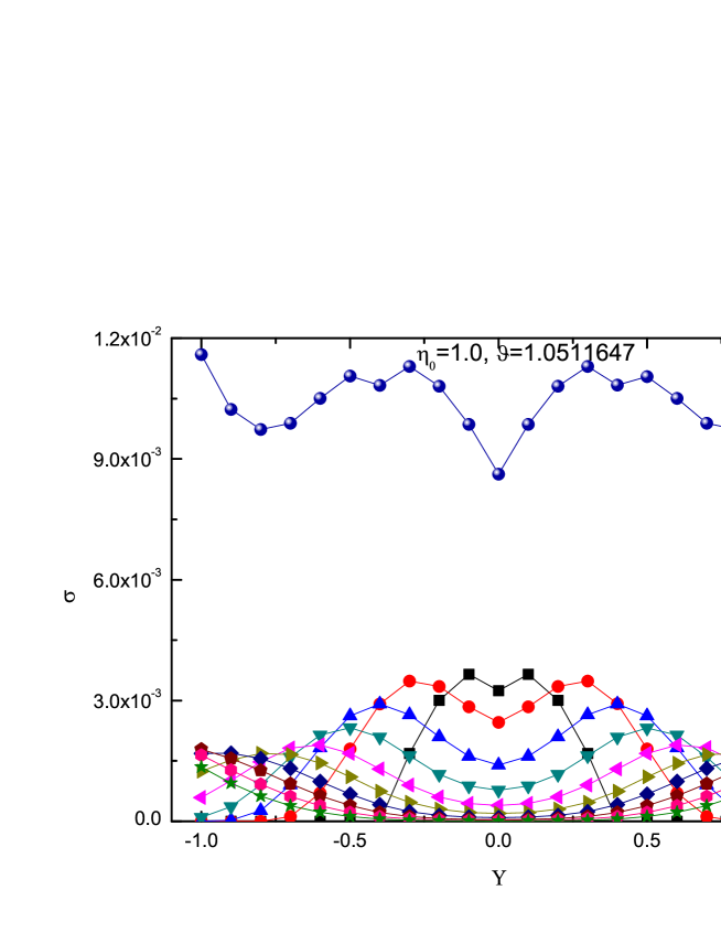
Figure 1: (Color online) The pair cross section $\bar{\sigma}_{N}$ for different number of photons dressed, i.e, from 6 to 30 and $\bar{\sigma}$, the summation of them, are plotted. Here, for example, $N=6$, represents the number of photons dressed from the laser field in the multi-photons process. $\eta_{0}$ and $\vartheta$ are the parameters fixed in the numerical simulation, while $\Upsilon$ is controlled. We only plot $\bar{\sigma}_{N}$ for $N\in\{6,7,\ldots,15\}$, and $\bar{\sigma}\approx\sum^{30}_{N=6}\bar{\sigma}_{N}$, because $\bar{\sigma}_{N}=0$ when $N=\{1,\ldots,5\}$. All other figures will have these adoptions unless otherwise specified.

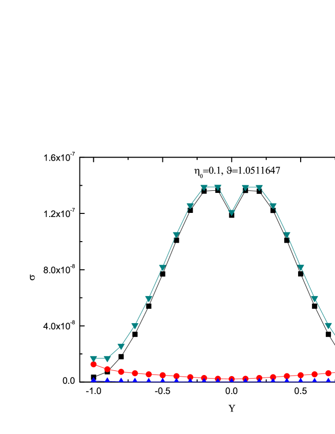
Figure 2: (Color online) Pair production $\bar{\sigma}_{N}$ and $\bar{\sigma}$ when $\eta_{0}=0.1$ and $\vartheta=1.0511647$. Here $\bar{\sigma}\approx\sum^{10}_{N=4}\bar{\sigma}_{N}$ and $\bar{\sigma}_{N}$ for $N\in\{7,\ldots,10\}$ have been omitted for their insignificance.

Surprisingly we can clearly see that the optimal polarization parameter $\Upsilon$ is $1.0$ or $-1.0$ rather than $0$ as thought by some people. On the other hand, the total production cross sections $\bar{\sigma}$ at $\Upsilon=0.3$, $0.4$ and $0.5$ are also very close to the optimal one. Furthermore, in the case of linear polarization the total pair production cross section is the smallest. It can be easily obtained that $\bar{\sigma}(\Upsilon=1)/\bar{\sigma}(\Upsilon=0)\approx 1.34$, and $\bar{\sigma}(\Upsilon=0.3)/\bar{\sigma}(\Upsilon=0)\approx 1.31$. These ratios indicate that the parameter $\Upsilon$ plays a very important role in directing the experiments to get more obvious and easy-detected results. We can also see that the numerical result is symmetric with respect to $\Upsilon=0$ as is expected by the theoretical requirement in Eq. (15).

Then we will unearth how the cross sections, $\bar{\sigma}_{N}$ and $\bar{\sigma}$, are influenced by $\eta_{0}$, the intensity of the polarized laser field. Usually the parameter $\vartheta$ is kept as a constant in experiments when $\eta_{0}$ is changed. Now we will calculate the pair production cross sections for different $\eta_{0}$. Here the strong constraint, $u_{N}=\frac{N\vartheta}{4(1+\eta^{2})}>1$, should be taken into account seriously, otherwise the integral of Eq. (15) would be zero. Given $\vartheta=1.0511647$ some numerical results with $\eta_{0}=0.1$, $0.5$ and $1.5$ are plotted in Fig. 2, Fig. 3 and Fig. 4, respectively. We also give the total cross sections $\bar{\sigma}$ for a series of different field intensities in Fig. 5 in order to see the effect of $\eta_{0}$.

Table 1: The relation between the optimal $\Upsilon$ which makes $\bar{\sigma}_{N}$ maximum and $N$ when $\eta_{0}=1.0$ and $\vartheta=1.0511647$. ”0.9/1.0” means that the cross section $\bar{\sigma}_{N}$ when $\Upsilon=0.9$ and $\Upsilon=1.0$ cannot be distinguished in our numerical simulation. Similar in Tables 2 and 3.

$N$	6	7	8	9	10	11	12	13	14	15
$|\Upsilon|$	0.1	0.3	0.4	0.5	0.6	0.7	0.9/1.0	1.0	1.0	1.0

As an example, in Table 1 we list the values of $|\Upsilon|$ corresponding to the optimal pair production cross section $\bar{\sigma}_{N}$ for different $N$ when $\vartheta=1.0511647$ and $\eta_{0}=1.0$. Actually, we have studied all the data we have got from numerical calculations, and find a fact that there exists a tendency: the larger $N$, the greater $|\Upsilon|$. This means that the polarized field becomes closer to the circular one for the optimal pair production $\bar{\sigma}_{N}$ as $N$ increases. This behavior is more obvious for smaller $\eta_{0}$ where $N$ is larger. Therefore, a dominant contribution to $\bar{\sigma}_{N}$ arises from $|\Upsilon|=1$ when $N$ is large. However, this conclusion for total pair production is not valid in general because the $N$-order cross section $\bar{\sigma}_{N}$ attributed to the total cross section decreases as $N$ increases. This point is also seen in Fig. 5, for example, where the optimal total pair production for $\eta_{0}=1.5$ is not at $|\Upsilon|=1$ but at $0.4$. It should be emphasized that for the total cross section there is a trade-off between $\eta_{0}$ and $\Upsilon$ which makes $\bar{\sigma}$ optimal.

Table 2: The relation between the optimal $\Upsilon$ which makes $\bar{\sigma}$ maximum and $\eta_{0}$ when $\vartheta=1.0511647$.

$\eta_{0}$	0.1	0.3	0.5	0.7	1.0	1.2	1.5
$|\Upsilon|$	0.1	0.1	1.0	1.0	1.0	0.3/0.4/0.5	0.4

Table 3: The relation between the optimal $\Upsilon$ which makes $\bar{\sigma}$ maximum and $\vartheta$ when $\eta_{0}=1.0$.

$\vartheta$	1.0511647	3.0	6.0	10.0	15.0	21.0	28.0	36.0	45.0	55.0
$|\Upsilon|$	1.0	0.5/0.6	0.6	0.3	0.3	0.3	0.3	0.2/0.3	0.2/0.3	0.2/0.3

On one hand, for smaller $\eta_{0}$ the main contribution to total $\bar{\sigma}$ comes from $\bar{\sigma}_{n_{0}}$ since other terms $(\bar{\sigma}_{N>n_{0}})$ decrease rapidly, see Fig. 2. In this situation the optimal polarization parameter approaches the linear one, see also Table 2 in the cases of $\eta_{0}=0.1$ and $0.3$. On the other hand, as $\eta_{0}$ increases to $\sim 1.0$, the field polarization parameter of optimal total pair production cross section becomes the circular one, $|\Upsilon|=1$. The same results are shown in Table 1 for very large $N$, because in these cases the terms of $\bar{\sigma}_{N>n_{0}}$ decrease more slowly so that the whole contribution from these large $N$ terms exceeds that from those small $N$ terms. This point can also be seen clearly in Fig. 1 and Fig. 3. However, as $\eta_{0}$ increases further a typical nonlinear feature arises between $|\Upsilon|$ and $\eta_{0}$ for the optimal pair creation. From Fig. 4 and Table 2 the trade-off between $|\Upsilon|$ and $\eta_{0}$ contribution to total cross section compels the optimal polarization to locate at about $|\Upsilon|=0.4$, which is between linear and circular polarizations for our studied field parameters.

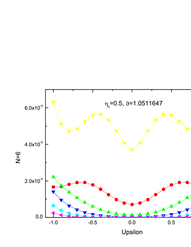
Figure 3: (Color online) Pair production $\bar{\sigma}_{N}$ and $\bar{\sigma}$ when $\eta_{0}=0.5$ and $\vartheta=1.0511647$. Here $\bar{\sigma}\approx\sum^{14}_{N=5}\bar{\sigma}_{N}$ and $\bar{\sigma}_{N}$ for $N\in\{5,11,\ldots,14\}$ have been omitted for their insignificance.

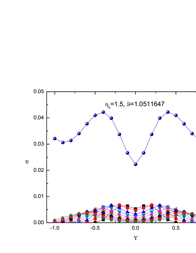
Figure 4: (Color online) Pair production $\bar{\sigma}_{N}$ and $\bar{\sigma}$ when $\eta_{0}=1.5$ and $\vartheta=1.0511647$. Here $\bar{\sigma}\approx\sum^{40}_{N=9}\bar{\sigma}_{N}$ and $\bar{\sigma}_{N}$ for $N\in\{19,\ldots,40\}$ have been omitted, but the contribution from them is not insignificant.

In a word, although the pair production cross section increases monotonically with laser field intensity, its optimal value depends strongly on laser field polarization, see Fig. 5. The former can be understood by the perturbation concept but the later can be recognized as the typical nonlinear interaction between fields and vacuum in QED, i.e. the laser dressed electrons/positrons colliding with a high energy photon.

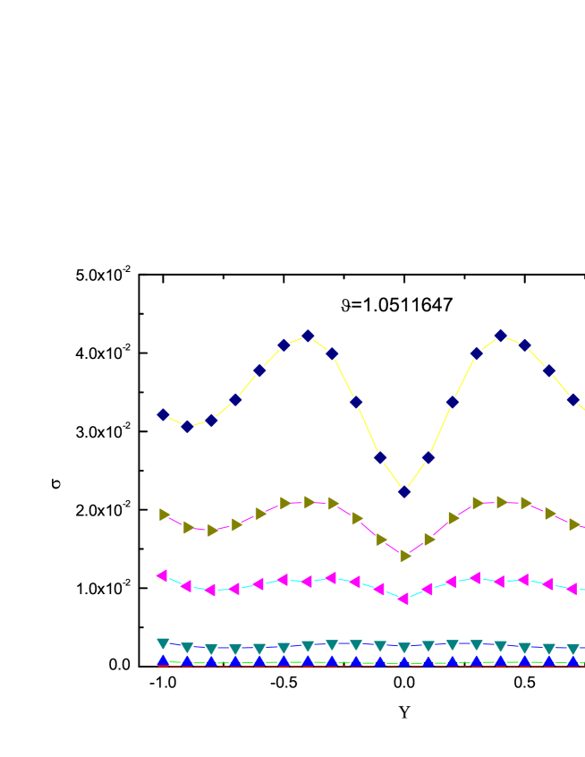
Figure 5: (Color online) All the total cross sections $\bar{\sigma}$ for different $\eta_{0}$ when $\vartheta=1.0511647$ are plotted in one figure to unearth more information.

III.2 Pair production cross section dependence on $\vartheta$

Besides two important parameters, $\Upsilon$ and $\eta_{0}$, the pair creation is also closely related to the parameter $\vartheta$. The problem, in fact, is how to tune the parameter $\vartheta$, to improve the pair production, given that $u_{N}=\frac{N\vartheta}{4(1+\eta^{2})}>1$. The idea is conformed with the physical picture as $\sqrt{\vartheta}=\sqrt{2(k^{{}^{\prime}}\cdot k)}/m_{0}$, which means the collision energy of two photons. Usually one believes that the larger $\vartheta$ is, the more likely the process of pair generation occurs. But things may not be so simple. We will find that the pair production will surely be greatly enhanced, in the first order, then begin to decrease in quantity when $\vartheta$ is bigger than a critical $\vartheta_{c}$, which again exhibits the nonlinear characteristic of QED process. Some values of $\vartheta$ are selected for fixed $\eta_{0}$, which are 3.0, 6.0, 10.0, 15.0, 21.0, 28.0, 36.0, 45.0 and 55.0 and the numerical results with $\vartheta=10.0,15.0,55.0$ are demonstrated graphically from Fig. 6 to Fig. 8. We also give all the total cross sections $\bar{\sigma}$ for different $\vartheta$ in Fig. 9 and Fig. 10 in order to make convenient comparisons with each other.

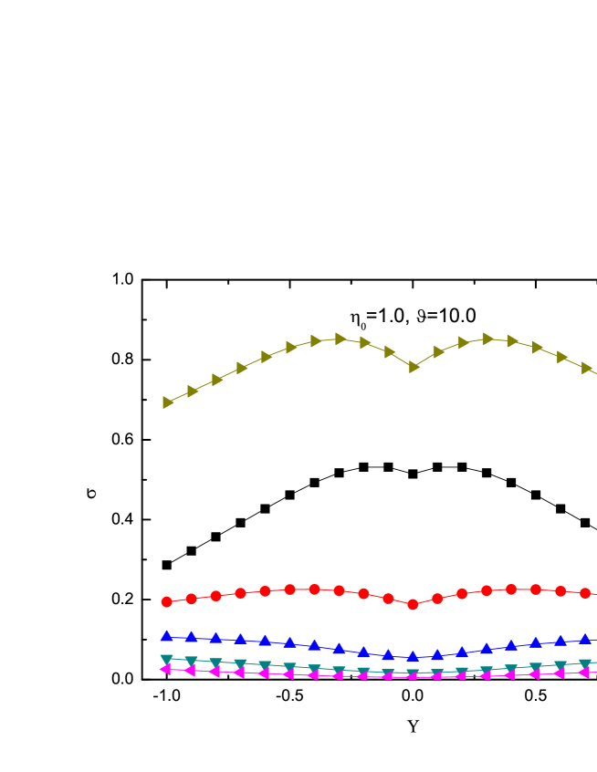
Figure 6: (Color online) Pair production $\bar{\sigma}_{N}$ and $\bar{\sigma}$ when $\eta_{0}=1.0$ and $\vartheta=10.0$. Here $\bar{\sigma}\approx\sum^{10}_{N=1}\bar{\sigma}_{N}$ and $\bar{\sigma}_{N}$ for $N\in\{6,\ldots,10\}$ have been omitted for their insignificance.

Now we will see how $\vartheta$ influences the pair creation. Firstly, from Fig. 9, we can see that the pair production is greatly enhanced with the increase of $\vartheta$ for fixed $\eta_{0}$, same behavior as shown in Ref. GrRe for the circularly polarized field. But it is not monotonically increasing with $\vartheta$ since the total cross section $\bar{\sigma}$ starts to decrease when $\vartheta\geq 15.0$ in our numerical results. The physical mechanism of this phenomenon seems difficult to grasp, however, a closer inspection of the integral of Eq. (15) shows that there exist two mathematic reasons for this counterintuitive phenomenon, i.e. the influence of Bessel functions and the inverse relation between the total cross section $\bar{\sigma}$ and $\vartheta$ in the coefficient $\frac{1}{\vartheta\eta^{2}}$. Certainly whether this phenomenon is kept in multiphoton perturbation regime, in which the higher order terms are included, or even in nonperturbation regime, is still an open problem. This difficult problem may be overcome in future possible theoretical calculations as well as more experiments.

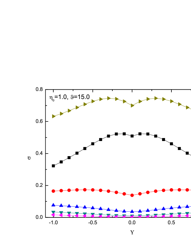
Figure 7: (Color online) Pair production $\bar{\sigma}_{N}$ and $\bar{\sigma}$ when $\eta_{0}=1.0$ and $\vartheta=15.0$. Here $\bar{\sigma}\approx\sum^{10}_{N=1}\bar{\sigma}_{N}$ and $\bar{\sigma}_{N}$ for $N\in\{6,\ldots,10\}$ have been omitted for their insignificance.

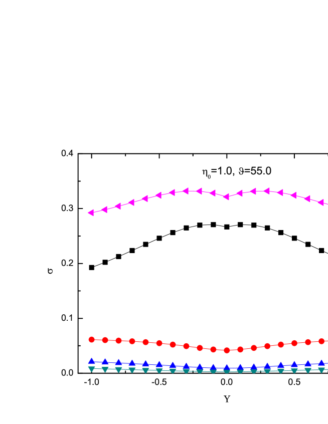
Figure 8: (Color online) Pair production $\bar{\sigma}_{N}$ and $\bar{\sigma}$ when $\eta_{0}=1.0$ and $\vartheta=55.0$. Here $\bar{\sigma}\approx\sum^{10}_{N=1}\bar{\sigma}_{N}$ and $\bar{\sigma}_{N}$ for $N\in\{5,\ldots,10\}$ have been omitted for their insignificance.

$\bar{\sigma}$ is a summation of different $\bar{\sigma}_{N}$ when $N$ is subject to $u_{N}>1.0$. Let us remember a fact that if the main contribution comes from the first term with least number $N=n_{0}$ then the optimal pair production is prone to the linearly polarized field. This is more obvious for larger $\vartheta$ as shown in Table 3. But there are some exceptions for smaller $\vartheta$, for example, $|\Upsilon|=1$ corresponds to parameter $\vartheta\approx 1.05$ in SLAC experiment case. More interesting, in our first order perturbation theory, when $\vartheta$ is large the pair production seems insensitive to the polarization parameter $\Upsilon$. From our numerical results we can see clearly, in Fig. 1, Fig. 9 and Fig. 10, that on one hand there is relatively large fluctuation of the cross section with respect to the polarization parameter for $\vartheta\in[1.05,21.0]$ and on the other hand there is indeed relatively small change of the cross section with respect to the polarization parameter $\Upsilon$ when $\vartheta\geq 28.0$. Although the main reason is unclear physically, the conclusion from numerical results is still very meaningful and useful. It provides an intuitive conclusion that when the collision energy of two photons is large enough usually one can directly choose the linearly or circularly polarized laser field, which is relatively easier to get in laboratories, for the pair production. With such special choices of polarization the cross section of the pair production does not differ from the optimal one greatly (less than 15% when $\vartheta\geq 36.0$, as shown in Fig. 10).

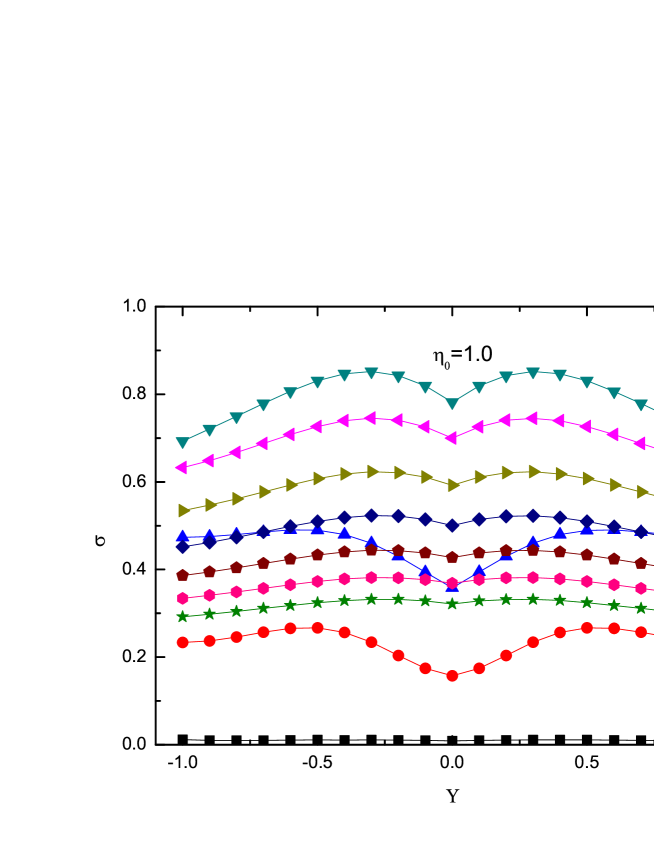
Figure 9: (Color online) All the total cross sections $\bar{\sigma}$ in different $\vartheta$ when $\eta_{0}=1.0$ are plotted in one figure to unearth more information. Here $\vartheta=1.0511647$ is shortened as $\vartheta=1.05$ in the figure.

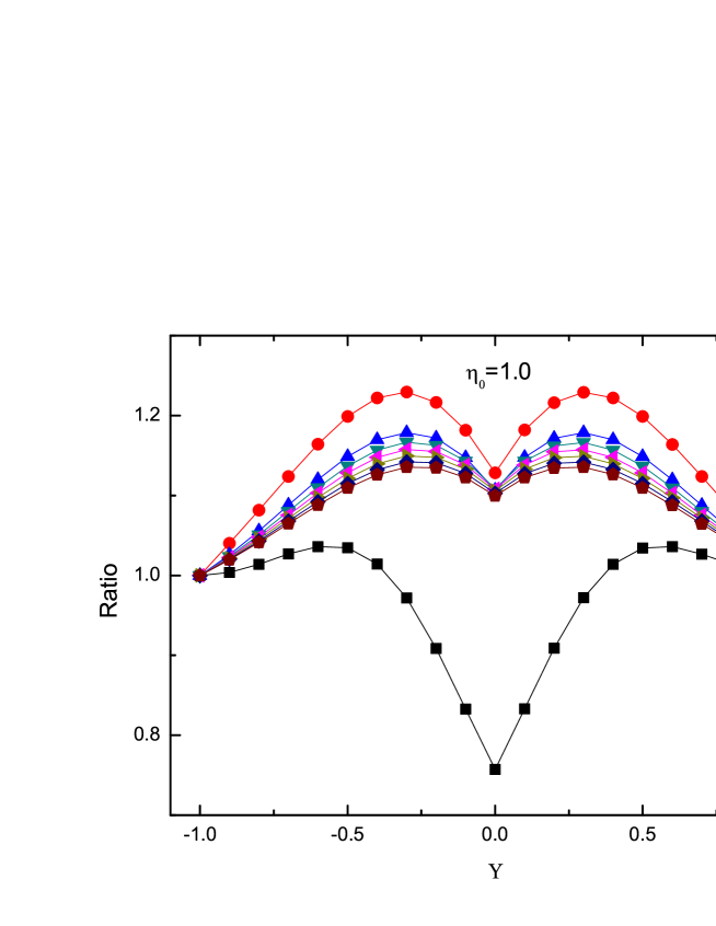
Figure 10: (Color online) This figure is corresponding to Fig. 9 and here ”Ratio” is the ratio of $\bar{\sigma}_{\Upsilon}$ and the corresponding $\bar{\sigma}$ of the circular in the same parameters $\vartheta$ and $\eta_{0}$. We have omitted the cases when $\vartheta=1.0511647,3.0$.

IV Discussions and conclusions

We have obtained the rigorous formula in the first order perturbation theory and performed thorough numerical computations for the pair production. Our numerical results for the parameters of the SLAC experiment have clearly manifested that the linear laser field is not the optimal one, but rather the circular one, although the partial cross section $\bar{\sigma}_{6}$ in the case of linear polarization is larger than that in the case of circular one. Surprisingly, neither linear nor circular but the elliptically polarized field corresponds to the optimal pair creation cross section in some cases shown in Table 2 and Table 3.

Our numerical results have also demonstrated that the leading contribution in the pair production comes from the first term subject to $u_{N}=\frac{N\vartheta}{4(1+\eta^{2})}>1.0$, when the polarization is nearly linear; moreover, things begin to change as larger $N$ is considered, since $\bar{\sigma}_{N}$ for larger $N$ is prone to the circular one. It might be the main reason that causes the balance between the linearly and the circularly polarized and also the reason of many nonlinear dependence of pair production on other system parameters. From our numerical results, we also see that when $\eta_{0}$ is large the contributions from $\bar{\sigma}_{N}$ with large $N$ are very important. While $\vartheta$ is large the contribution from $\bar{\sigma}_{N}$ with large $N$ are not so important. For example, given $\eta_{0}=1.0$, when we calculate the total cross section for $\vartheta=1.0511647$, at least $\sum^{30}_{N=6}\bar{\sigma}_{N}$ is used; however, for $\vartheta\geq 6.0$, summation by $\sum^{10}_{N=1}\bar{\sigma}_{N}$ as an approximation of $\bar{\sigma}$ is already good enough. By the way for $\eta_{0}=1.5$ and $\vartheta=1.0511647$ a calculation by $\sum^{40}_{N=9}\bar{\sigma}_{N}$ is needed.

We have exhibited the abundance phenomena in the process of photon-multiphoton reaction that the laser field polarization plays a key role in optimal pair production when the other parameters are fixed, which can be seen from Fig. 1 to Fig. 10 and three tables. Our work may provide some understanding about some previous experimental phenomena Burke ; Altarelli and also direction for future experiments. Although a great effort has been made to understand the polarization effect on the pair production, there still remain some open problems to be solved, especially the physical mechanism behind the complex calculational formulae. We conjecture that there may be nonlinear resonance or/and interference terms appeared in different modes of scattering matrix elements for the transition amplitude which would enhance or reduce the pair production cross section in different polarization cases. However, more theoretical and experimental research are still needed in the future to have a deeper understanding of vacuum decay in ultrastrong laser field to create electron-positron pairs, which serves as an important test for nonlinear QED.

References

• (1) D. Strickland and G. Mourou, Opt. Commum. 56, 219(1985).
• (2) G. Mourou, T.Tajima and S. Bulanov, Rev. Mod. Phys. 78, 309(2006).
• (3) D. L. Burke et al., Phys. Rev. Lett. 79, 1626(1997).
• (4) C. Bamber et al., Phys. Rev. D 60, 092004 (1999).
• (5) http://www.extreme-light-infrastructure.eu/
• (6) J. Schwinger, Phys. Rev. 82, 664(1951).
• (7) D. M. Volkov, Z. Phys. 94, 250(1935).
• (8) F. Sauter, Z. Phys. 69, 742(1931).
• (9) S. P. Kim and D. N. Page, Phys. Rev. D 65, 105002(2002).
• (10) G. V. Dunne and C. Schubert, Phys. Rev. D 72, 105004(2005).
• (11) H. Gies and K. Klingmüller, Phys. Rev. D 72, 065001(2005).
• (12) G. V. Dunne Q. H. Wang, H. Gies and C. Schubert, Phys. Rev. D 73, 065028(2006).
• (13) C. Mlüler, A. B. Voitkiv and N. Grün, Phys. Rev. A 67, 063407(2003).
• (14) C. Deneke and C. Müller, Phys. Rev. A 78, 033431(2008).
• (15) C. Müller, K. Z. Hatsagortsyan and C. H. Keitel, Phys. Rev. A 78, 033408(2008).
• (16) H. Y. Hu, C. Müller and C. H. Keitel, Phys. Rev. Lett. 105, 080401(2010).
• (17) M. S. Marinov and V. S. Popov, Sov. J. Nucl. Phys. 16, 449(1973).
• (18) S. S. Bulanov, Phys. Rev. E 69, 036408(2004).
• (19) H. R. Reiss, J. Math. Phys. 3, 59(1962).
• (20) A. I. Nikishov and V. I. Ritus, Sov. Phys. JETP 19, 529(1964).
• (21) M. Altarelli et al., Technical Design Report of the European XFEL, DESY 2006-097(http://www.xfel.net).
• (22) W. Greiner and J. Reinhardt, Quantum Electrodynamics, p. 222-232 (Springer-Verlag Berlin Heidelberg, Fourth Edition 2009).
• (23) V. B. Berestetskii, E. M. Lifshitz and L. P. Pitaevskii, Quantum Electrodynamics (Pergamon, Oxford, 1982).
• (24) W. H. Press, S. A. Teukolsky, W. T. Vetterling and B. P. Flannery, Numerical Recipes in C (Cambridge University Press, Cambridge, 1992).