Microstructure identification via detrended fluctuation analysis of ultrasound signals

Abstract

We describe an algorithm for simulating ultrasound propagation in random one-dimensional media, mimicking different microstructures by choosing physical properties such as domain sizes and mass densities from probability distributions. By combining a detrended fluctuation analysis (DFA) of the simulated ultrasound signals with tools from the pattern-recognition literature, we build a Gaussian classifier which is able to associate each ultrasound signal with its corresponding microstructure with a very high success rate. Furthermore, we also show that DFA data can be used to train a multilayer perceptron which estimates numerical values of physical properties associated with distinct microstructures.

I Introduction

Much attention has been given to the problem of wave propagation in random media by the condensed-matter physics community, especially in the context of Anderson localization and its analogs Anderson (1958); Hodges (1982); Baluni and Willemsen (1985); Gavish and Castin (2005); Bahraminasab et al. (2007). A hallmark of these phenomena is the fact that randomness induces wave attenuation by energy confinement, even in cases where dissipation can be neglected. The interplay of energy confinement and randomness gives rise to noisy but correlated signals, for instance, in the case of acoustic pulses propagating in inhomogeneous media.

It has long been known that the correlations in a time series hide relevant information on its generating dynamics. In a pioneering paper, Hurst Hurst (1951) introduced the rescaled-range analysis of a time series, which measures the power-law growth of properly rescaled fluctuations in the series as one looks at larger and larger time scales $\tau$. The associated Hurst exponent $H$ governing the growth of such fluctuations is able to gauge memory effects on the underlying dynamics, offering insight into its character. The presence of long-term memory leads to a value of the exponent $H$ which deviates from the uncorrelated random-walk value $H=1/2$, persistent (antipersistent) behavior of the time series yielding $H>1/2$ ($H<1/2$). Additionally, a crossover at a time scale $\tau_{\times}$ between two regimes characterized by different Hurst exponents may reveal the existence of competing ingredients in the dynamics, and in principle provides a signature of the associated system. This forms the base of methods designed to characterize such systems Matos et al. (2004), if one is able to obtain reliable estimates of the Hurst exponents. This is in general a difficult task, as even local trends superposed on the noisy signal may affect the rescaled-range analysis, obscuring the value of $H$. A related exponent, $\alpha$, defined through detrended fluctuation analysis (DFA) Peng et al. (1994), can be used instead.

Actually, the characteristics of exponents and crossovers observed in the DFA curves associated with various types of data series have been extensively used to distinguish between the systems producing such series. Examples include coding versus noncoding DNA regions Peng et al. (1994); Ossadnik et al. (1994), healthy versus diseased subjects as regards cardiac Goldberger et al. (2002), neurological Hausdorff et al. (2000); Hwa and Ferree (2002) and respiratory function Peng et al. (2002), and ocean versus land regions as regards temperature variations Fraedrich and Blender (2003). However, there are many instances in which these characteristics are not clearcut and the DFA curves exhibit a more complex dependence on the time scale. In such cases, it has been shown that pattern recognition tools Webb (2002) can help the identification of relevant features, greatly improving the success of classification tasks Vieira et al. (2008, 2009); de Moura et al. (2009); Vieira et al. (2010).

In the present work, we investigate the possibility of extracting information on the nature of inhomogeneities by analyzing fluctuations in time series associated with ultrasound propagation in random media. A hint that this possibility is real was provided by the fact that the crossover features of DFA and Hurst analysis curves from backscattered ultrasound signals revealed signatures of the microstructure of cast-iron samples Matos et al. (2004). Here, in order to perform a systematic study, we resort to simulating the propagation of ultrasound pulses in one-dimensional media with distinct microstructures, defined by probability distributions of physical properties such as domain size, density and sound velocity. Although this choice of geometry cannot allow for the full phenomenology of sound propagation (such as mode conversion from transverse to longitudinal sound waves), it makes it possible to generate large quantities of simulated data, which are important in order to assess the generalizability of our reported results. Moreover, it approximately describes normal propagation of sound waves in layered media.

The paper is organized as follows. In Sec. II we present the artificial microstructures we produced, as well as a sketch of the simulation technique; a detailed description is relegated to Appendix A. In Sec. III we describe the method of detrended fluctuation analysis and its results when applied to our simulated signals. Then, in Sec. IV, we report on an automated classifier which is able to associate, with a very high success rate, the DFA curves with the corresponding microstructure. Furthermore, we show in Sec. V that the DFA curves can be used to train a neural network which predicts numerical values of physical properties associated with different microstructures. We close the paper by presenting a summary in Sec. VI.

II Simulating ultrasound propagation

We are interested in studying ultrasound propagation along a one-dimensional medium of width $W$, with a pulse generated in a transducer located at one end of the system. Since the medium consists of many different domains, with possibly different physical properties (density and sound velocity), in general the pulse will be scattered as it propagates towards the opposite end, where it will be reflected. Information on the microstructure is in principle hidden in the scattered signal, which is registered in the transducer as it arrives.

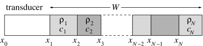
Figure 1: Sketch of the geometry used in simulating ultrasound propagation in an inhomogeneous medium. See main text for labels.

The domains are labeled by an index $j$, so that domain $j$ extends between $x_{j}$ and $x_{j+1}$, and is characterized by its density $\rho_{j}$ and its sound velocity $c_{j}$. (See Figure 1.) For the one-dimensional geometry employed here, the solution of the wave equation can be carried out semi-analytically, as detailed in Appendix A. For a given choice of physical parameters $\left\{\rho_{j},c_{j}\right\}$ of the various domains, the displacement field inside the medium, as a function of position $x$ and time $t$, can be written as

$$\Phi\left(x,t\right)=\sum_{k}\phi_{k}X_{k}\left(x\right)\cos\left(\omega_{k}t\right),$$ (1)

where $k$ labels the different eigenfrequencies $\omega_{k}$, the function $X_{k}\left(x\right)$ is explicitly given by

$$X_{k}\left(x\right)=A_{jk}\cos\left(\omega_{k}x/c_{j}\right)+B_{jk}\sin\left(\omega_{k}x/c_{j}\right),$$ (2)

with $j$ such that $x_{j}\leq x<x_{j+1}$, and the coefficients $A_{jk}$ and $B_{jk}$ are determined from boundary conditions at the interfaces separating contiguous domains, while the weights $\phi_{k}$ are derived from the initial condition $\Phi\left(x,0\right)$. Here we choose an initial pulse contained entirely inside the transducer, with a form given by

$$\Phi\left(x,0\right)=\Phi_{0}e^{-\gamma\left(x-x_{\mathrm{trans}}\right)}\sin\left[\frac{2\pi f\left(x-x_{\mathrm{trans}}\right)}{c_{\mathrm{trans}}}\right],$$ (3)

for $x$ inside the transducer, and $\Phi\left(x,0\right)=0$ otherwise, where $\Phi_{0}$ is an amplitude, $f$ is the reference frequency of the transducer, $c_{\mathrm{trans}}$ is the sound velocity inside the transducer, $x_{\mathrm{trans}}$ is the position of the left end of the transducer, and $\gamma$ is a “damping” factor, introduced so as to make the pulse resemble those produced by a real transducer. In this work, we use $f=10\,\mathrm{MHz}$, $c_{\mathrm{trans}}=5800\,\mathrm{m/s}$, and $\gamma=129.31\,\mathrm{m}^{-1}$, for a transducer of length $2.32\,\mathrm{cm}$, in which 4 wavelengths of the pulse can fit. The density inside the transducer is chosen as $\rho_{\mathrm{trans}}=2600\,\mathrm{kg/m}^{3}$ (about the density of quartz). We take into account in Eq. (1) all eigenfrequencies $\omega_{k}$ smaller than $\omega_{\mathrm{max}}=16\times 2\pi f$, corresponding to $16$ times the reference angular frequency of the transducer. We checked that halving the value of $\omega_{\mathrm{max}}$ has no relevant effect on the results we report below.

From the displacement field, the sound pressure increments can be calculated as

$$p\left(x,t\right)=\rho_{j}c_{j}^{2}\frac{\partial\Phi\left(x,t\right)}{\partial x}=\rho_{j}c_{j}^{2}\sum_{k}\phi_{k}X_{k}^{\prime}\left(x\right)\cos\left(\omega_{k}t\right),$$ (4)

again with $j$ such that $x_{j}\leq x<x_{j+1}$. The ultrasound signals we keep correspond to time series of the displacement and the pressure increments captured at the right end of the transducer, with a sampling rate of $50\,\mathrm{MHz}$. Each time series contains $2048$ points, corresponding to about $4\times 10^{-5}$ seconds.

Microstructure	Average domain size ($\mathrm{m}$)	Average density ($\mathrm{kg}/\mathrm{m}^{3}$)
1	$1.4\times 10^{-5}$	$7900$
2	$5.6\times 10^{-5}$	$7900$
3	$2.24\times 10^{-4}$	$7900$
4	$8.96\times 10^{-4}$	$7900$
5	$1.4\times 10^{-5}$	$6959$
6	$5.6\times 10^{-5}$	$6959$
7	$2.24\times 10^{-4}$	$6959$
8	$8.96\times 10^{-4}$	$6959$
9	$1.4\times 10^{-5}$	$6130$
10	$5.6\times 10^{-5}$	$6130$
11	$2.24\times 10^{-4}$	$6130$
12	$8.96\times 10^{-4}$	$6130$
13	$1.4\times 10^{-5}$	$5400$
14	$5.6\times 10^{-5}$	$5400$
15	$2.24\times 10^{-4}$	$5400$
16	$8.96\times 10^{-4}$	$5400$

Table 1: Average values of physical properties for the 16 different microstructures used in this work. The sound velocity is fixed at $5900\,\mathrm{\mathrm{m}/\mathrm{s}}$ in all cases.

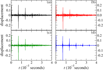
Figure 2: Typical simulated ultrasound signals from microstructures $1$ (a) to $4$ (d).

We work here with 16 different choices of microstructure, combining 4 different average domain sizes and 4 different average densities, with characteristics detailed in Table 1. The actual size and density of a domain are chosen from Gaussian probability distributions with a standard deviation of 10% the average value for the size, and of 2.5% the average value for the density. For each of the $16$ microstructures, we obtained signals from $100$ different disorder realizations, with a total of $1600$ signals. Our aim is to identify the microstructure based on the analysis of the ultrasound signal. Since we keep the average system size fixed at $W=2\,\mathrm{cm}$, we assume the same sound velocity ($5900\,\mathrm{\mathrm{m}/\mathrm{s}}$) for all microstructures, so that the time intervals between signal peaks do not trivially reveal the microstructure type. Typical signals are shown in Fig. 2. Notice that fluctuations in the signals increase from microstructure $1$ to microstructure $2$, and decrease for microstructures $3$ to $4$. This nonmonotonic behavior of the fluctuations as a function of average domain size is due to the fact that the average time needed for the wave to propagate through a domain in microstructure $2$ is about $1/f=10^{-5}\,\mathrm{s}$, thus maximizing scattering.

III Detrendend fluctuation analysis

The detrended fluctuation analysis (DFA), introduced by Peng et al. Peng et al. (1994), calculates the detrended fluctuations in a time series as a function of a time-window size $\tau$. The detrending comes from fitting the integrated time series inside each time window to a polynomial, and calculating the average variance of the residuals. Explicitly, the method works as follows. A time series $\left\{u_{i}\right\}$ of length $M$ is initially integrated, yielding a new time series $y_{j}$,

$$y_{j}=\sum_{i=1}^{j}\left(u_{i}-\left\langle u\right\rangle\right),$$ (5)

the average $\left\langle u\right\rangle$ being taken over all points,

$$\left\langle u\right\rangle=\frac{1}{M}\sum_{i=1}^{M}u_{i}.$$ (6)

For each time window $I_{k}$ of size $\tau$, the points inside $I_{k}$ are fitted by a polynomial of degree $l$ (which we take in this work to be $l=1$, i.e. a straight line), yielding a local trend $\tilde{y}_{j}$, corresponding to the ordinate of the fit. The variance of the residuals is calculated as

$$f_{k}^{2}\left(\tau\right)=\frac{1}{\tau-1}\sum_{i\in I_{k}}\left(y_{j}-\tilde{y}_{j}\right)^{2},$$ (7)

and $f_{k}\left(\tau\right)$ is averaged over all intervals to yield the detrended fluctuation $F\left(\tau\right)$,

$$F\left(\tau\right)=\frac{1}{M-\tau+1}\sum_{k}f_{k}\left(\tau\right),$$ (8)

$M-\tau+1$ being the number of time windows of size $\tau$ in a time series with $M$ points. As defined here, $\tau$ is the (integer) number of points inside a time window, the time increment between consecutive points corresponding to the inverse sampling rate, $2\times 10^{-8}\,\mathrm{s}$.

Notice that here, besides using overlapping time windows, we also calculate the variance of the residuals inside each window, in a similar spirit to what is done for the detrended cross-correlation analysis of Ref. Podobnik and Stanley (2008). This approach is slightly distinct from the original scheme of Ref. Peng et al. (1994), where nonoverlapping time windows are employed, and the variance is calculated for the whole time series. When applied to fractional Brownian motion Addison (1997) characterized by a Hurst exponent $H$, both approaches yield the same exponent within numerical errors. Interestingly, the performance of the classifier described in Sec. IV, however, is significantly improved by our approach.

When applied to a time series generated by a process governed by a single dynamics, as for instance in fractional Brownian motion Addison (1997), DFA yields a function $F\left(\tau\right)$ following a power-law behavior,

$$F\left(\tau\right)\sim C\tau^{\alpha},$$ (9)

in which $C$ is a constant and $\alpha$ is an exponent which is related to the Hurst exponent $H$, measuring memory effects on the dynamics. If persistent (antipersistent) behavior of the time series is favored, $\alpha$ is larger (smaller) than $1/2$.

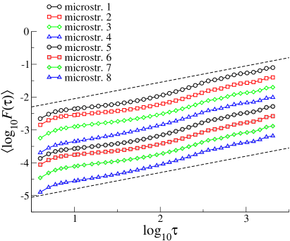
Figure 3: Average DFA curves for 8 different microstructures as a function of the the time-window size $\tau$ (offset vertically for clarity). The dashed lines have slope $1/2$.

As shown in Fig. 3, for a subset of $8$ microstructures, the curves of $F\left(\tau\right)$ calculated from the displacement fields of simulated ultrasonic signals do not conform in general to a power-law behavior, so that the exponent $\alpha$ is ill-defined, except perhaps for microstructures $4$ and $8$, characterized by the largest average domain sizes, which yield exponents approaching the uncorrelated random-walk value $\alpha=1/2$. This same value can be approximately identified for the other microstructures if the analysis is restricted to a range of time-window sizes $\tau$ such that $\log_{10}\tau\geq 2.5$, which correspond to time scales greater than $6.3\times 10^{-6}\,\mathrm{s}$, compatible with the time $6.78\times 10^{-6}\,\mathrm{s}$ needed for the pulse to travel across the medium and return to the transducer. At shorter time scales, scattering of the waves at the interfaces between domains introduces large interference effects leading to the antipersistent behavior revealed by the $F\left(\tau\right)$ curves. Such effects, as expected, are stronger for microstructures $1$, $2$, $5$, and $6$, characterized by smaller average domain sizes. Even shorter time-window sizes, $\log_{10}\tau\lesssim 0.7$, probe time scales inferior to the inverse frequency of the pulse, $1/f=10^{-7}\,\mathrm{s}$, and, as expected, point to a locally persistent behavior of the time series.

Instead of attempting to correlate the signals with the microstructures based on a manual identification of the various aspects of the curves, we resort to pattern recognition tools Webb (2002). To this end, we define for each signal $i$ a DFA vector $\mathbf{x}_{i}$ whose components correspond to the values of the function $F\left(\tau\right)$ at a fixed set $\{\tau_{j}\}$ of window sizes. Here we build $\{\tau_{j}\}$ from the integer part of the integer powers of $2^{1/4}$, from $4$ to $2048$, comprising $37$ different values of $\tau$.

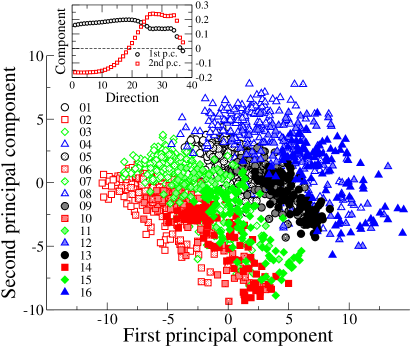
Figure 4: Projection of the DFA vectors on the plane defined by the first two principal components of the data, corresponding to the eigenvectors of the covariance matrix associated with the two largest eigenvalues. Inset: vector components of the eigenvectors for each of the $37$ directions.

A visualization of the DFA vectors is hindered by their high number of components, $n=37$. However, a principal-component analysis Webb (2002) can reveal the directions along which the data for all $1600$ vectors is most scattered. This is done by projecting each vector along the principal components, corresponding to the eigenvectors of the covariance matrix

$$\bm{\Sigma}=\frac{1}{N}\sum_{i}\left(\mathbf{x}_{i}-\bm{\mu}\right)\left(\mathbf{x}_{i}-\bm{\mu}\right)^{T},$$ (10)

in which the summation runs over all $N=1600$ DFA (column) vectors $\mathbf{x}_{i}$, while $\bm{\mu}$ is the average vector,

$$\bm{\mu}=\frac{1}{N}\sum_{i}\mathbf{x}_{i}.$$ (11)

The eigenvectors are arranged in decreasing order of their respective eigenvalues. The first principal component thus corresponds to the direction accounting for the largest variation in the data, the second principal component to the second largest variation, etc. Figure 4 shows projections of all DFA vectors for displacements on the plane defined by the first two principal components, revealing at the same time a clustering of the data for each microstructure and a considerable superposition of the data for microstructures which differ only by average density (microstructures $1$, $5$, $9$, and $13$, for instance). Although this superposition is in part an artifact of the two-dimensional projection, it is not satisfactorily eliminated when the other directions are taken into account. Accordingly, attempts at associating a vector $\mathbf{x}_{i}$ to the microstructure whose average vector is closer to $\mathbf{x}_{i}$ lead to an error rate of about $42\%$. However, as discussed in the next Section, a more sophisticated approach considerably improves the classification performance.

Notice that, as shown in the inset of Fig. 4, special features of the first two eigenvectors of the covariance matrix are associated with directions $26$ and above, along which the components of the first (second) eigenvector have typically smaller (larger) absolute values than along other directions. Moreover, the components of the second eigenvector along directions $1$ to $5$ also have locally larger absolute values. In fact, direction $5$ is connected with the inverse frequency $1/f$, and directions above $26$ are associated with time-window sizes such that $\log_{10}\tau>2.5$, again pointing to the special role played by these time scales in differentiating the various microstructures.

IV Gaussian discriminants

We first want to check whether it is possible to build an efficient automated classifier which is able to assign a signal to one of the microstructures, based on the corresponding DFA vector. Attempts at assigning a DFA vector $\mathbf{x}$ to the microstructure (or class, in the language of pattern recognition) whose average vector lies closer to $\mathbf{x}$ lead to many classifications due to the fact that the average vectors of similar microstructures (such as $1$ and $5$) are close to one another. As a classification based solely on distance disregards additional information provided by the probability distributions of the DFA vectors obtained from each microstructure, whose variances along different directions can exhibit different profiles, here we follow an approach to discrimination based on estimates of those distributions.

Our task is to estimate the probability $P\left(\omega_{j}|\mathbf{x}\right)$ that a given vector $\mathbf{x}$ belongs to class $\omega_{j}$, $j\in\left\{1,2,\ldots,C\right\}$. (In our case, of course, $C=16$.) From Bayes’ theorem, this probability can be written as

$$P\left(\omega_{j}|\mathbf{x}\right)=\frac{P\left(\mathbf{x}|\omega_{j}\right)P\left(\omega_{j}\right)}{P\left(\mathbf{x}\right)},$$ (12)

where $P\left(\mathbf{x}|\omega_{j}\right)$ is the probability that a sample belonging to class $\omega_{j}$ produces a vector $\mathbf{x}$, $P\left(\omega_{j}\right)$ is the prior probability of class $\omega_{j}$ occurring, and $P\left(\mathbf{x}\right)$ is the prior probability of vector $\mathbf{x}$ occurring. Once $P\left(\omega_{j}|\mathbf{x}\right)$ is known for all classes $\omega_{j}$, we assign vector $\mathbf{x}$ to class $\omega_{j}$ if

$$P\left(\omega_{j}|\mathbf{x}\right)>P\left(\omega_{k}|\mathbf{x}\right),\quad\mbox{for all }k\neq j.$$

Since $P\left(\mathbf{x}\right)$ is class-independent, and thus irrelevant to the decision process, the problem of calculating $P\left(\omega_{j}|\mathbf{x}\right)$ reduces to estimating $P\left(\mathbf{x}|\omega_{j}\right)$ and $P\left(\omega_{j}\right)$.

Among the various possibilities for the estimation of $P\left(\mathbf{x}|\omega_{j}\right)$, we choose to work with normal-based quadratic discriminant functions Webb (2002), derived as follows. We assume that $P\left(\mathbf{x}|\omega_{j}\right)$ has the Gaussian form

$$P\left(\mathbf{x}|\omega_{j}\right)=\frac{1}{\left(2\pi\right)^{\frac{n}{2}}\left|\bm{\Sigma}_{j}\right|^{\frac{1}{2}}}\exp\left[-\frac{1}{2}\left(\mathbf{x}-\bm{\mu}_{j}\right)^{T}\bm{\Sigma}_{j}^{-1}\left(\mathbf{x}-\bm{\mu}_{j}\right)\right],$$ (13)

where $n$ is the number of components of $\mathbf{x}$, while $\bm{\mu}_{j}$ and $\bm{\Sigma}_{j}$ are the average vector and the covariance matrix of class $\omega_{j}$. By selecting a subset of the available vectors to form a training set $\left\{\mathbf{x}_{i}\right\}$, unbiased maximum-likelihood estimates of $\bm{\mu}_{j}$ and $\bm{\Sigma}_{j}$ are provided by

$$\hat{\bm{\mu}}_{j}=\frac{1}{\mathcal{N}_{j}}\sum_{i\in\omega_{j}}\mathbf{x}_{i}$$ (14)

and

$$\bm{\hat{\Sigma}}_{j}=\frac{1}{\mathcal{N}_{j}-1}\sum_{i\in\omega_{j}}\left(\mathbf{x}_{i}-\hat{\bm{\mu}}_{j}\right)\left(\mathbf{x}_{i}-\hat{\bm{\mu}}_{j}\right)^{T},$$ (15)

with $\mathcal{N}_{j}$ the number of vectors in the training set belonging to class $\omega_{j}$. The decision process then corresponds to assigning a vector $\mathbf{x}$ to class $\omega_{j}$ if $g_{j}\left(\mathbf{x}\right)>g_{k}\left(\mathbf{x}\right)$ for all $k\neq j$, where

$$g_{j}\left(\mathbf{x}\right)=\ln\hat{P}\left(\omega_{j}\right)-\frac{1}{2}\ln\left|\bm{\hat{\Sigma}}_{j}\right|-\frac{1}{2}\left(\mathbf{x}-\hat{\bm{\mu}}_{j}\right)^{T}\bm{\hat{\Sigma}}_{j}^{-1}\left(\mathbf{x}-\hat{\bm{\mu}}_{j}\right),$$ (16)

an estimate of $P\left(\omega_{j}\right)$ being given by

$$\hat{P}\left(\omega_{j}\right)=\frac{\mathcal{N}_{j}}{\sum_{k=1}^{C}\mathcal{N}_{k}}.$$ (17)

Microstructure	Success rate	Misclassifications
1	98.6 (0.3)	5: 1.4
2	98.7 (0.2)	6: 1.3
3	99.6 (0.1)	4: 0.1    7: 0.3
4	99.0 (0.2)	8: 1.0
5	99.1 (0.2)	1: 0.4   9: 0.5
6	99.8 (0.1)	2: 0.1   10: 0.1
7	98.8 (0.2)	3: 1.13    8: 0.04   11: 0.03
8	97.0 (0.4)	4: 2.9   12: 0.1
9	99.5 (0.1)	5: 0.5
10	99.8 (0.1)	14: 0.2
11	99.6 (0.1)	7: 0.3   15: 0.1
12	99.4 (0.2)	8: 0.6
13	99.7 (0.1)	9: 0.3
14	100	none
15	100	none
16	99.1 (0.2)	12: 0.9

Table 2: Average performance of the classifier when applied to the testing vectors built from displacements, calculated over $100$ sets of training and testing vectors. For the second column, bold numbers indicate the percentage of vectors which were correctly classified, figures in parenthesis corresponding to the standard deviations. The third column registers average misclassification rates (in the first row, ‘5: 1.4’ indicates that 1.4% of vectors belonging to microstructure 1 were misclassified as belonging to microstructure 5).

First we tested the classifier by using all the $1600$ DFA vectors for displacements as the training set. This yields functions $g_{k}\left(\mathbf{x}\right)$ that are able to correctly classify all vectors, a flawless performance. In order to evaluate the generalizability of the classifier results, we randomly selected $80\%$ ($1280$) of the $1600$ available vectors to define the training set, using the remaining vectors in the testing stage, and took averages over $100$ distinct choices of training and testing sets. When the training vectors were fed back to the classifier, as a first step toward validation, again no vectors were misclassified. Table 2 summarizes the average performance of the classifier when applied to the testing vectors built from the DFA analysis of the displacement signals. Notice that the maximum average classification error corresponds to $3\%$, for microstructure $8$. The overall testing error, taking into account all classes, corresponds to $0.8\%$. Misclassifications almost exclusively involve assigning a vector to a microstructure with the correct average domain size but different average density (e.g. microstructures $4$ or $12$ instead of $8$), with very few cases involving the same density but with a different although closest average domain size (microstructure $8$ instead of $7$). This fact can be used to build a classifier which groups vectors into 4 classes, according to the average domain size of the corresponding microstructures, with no misclassifications. A similar classifier targeting average densities rather than average domain sizes shows only a very small misclassification rate of $0.01\%$.

Interestingly, processing the displacement signals according to the original DFA recipe of Ref. Peng et al. (1994) leads to an inferior performance for microstructure classification, with an average error of $29\%$, but now most errors involve vectors being assigned to classes with the same density as that of the correct microstructure. A classifier which groups vectors according to the average density of the corresponding microstructures achieves a misclassification rate of only $2\%$.

The efficiency of the classifiers is dependent on the choice of values of the time-window sizes. For instance, in the 16-class case, restricting the values of $\tau_{j}$ to the powers of $2$ doubles the overall testing error, to around $1.7\%$, while expanding $\left\{\tau_{j}\right\}$ to the integer parts of the powers of $2^{1/8}$ leads to a much larger overall testing error of $24\%$. Choosing $\left\{\tau_{j}\right\}$ as the integer parts of the powers of $2^{1/2}$ actually leads to a slightly smaller overall testing error of $0.6\%$, but a few training errors also occur. Thus, our choice of $\left\{\tau_{j}\right\}$ from the integer parts of the powers of $2^{1/4}$ seems to be close to optimal. In contrast, performing the detrended fluctuation analysis according to the original recipe of Ref. Peng et al. (1994) leads to a minimum overall testing error of $28\%$ as the values of the time-window sizes are varied.

Microstructure	Success rate	Misclassifications
1	97.6 (0.4)	5: 1.6
2	83.5 (1.0)	6: 16.2
3	88.9 (0.8)	7: 11.0
4	91.7 (0.6)	8: 8.2
5	93.6 (0.6)	1: 1.2   6:2.7   9: 2.3
6	80.9 (1.1)	2: 10.5   10: 8.5
7	81.6 (1.0)	3: 12.2    11: 5.2
8	92.0 (0.7)	4: 5.1   12: 2.8
9	93.9 (0.6)	5: 3.3   10: 2.5
10	85.7 (0.9)	6: 9.3   14: 4.6
11	86.5 (0.9)	7: 8.6   15: 4.8
12	86.3 (0.9)	8: 11.2    16: 2.3
13	99.9 (0.1)	9: 0.1
14	95.2 (0.5)	10: 4.8
15	94.3 (0.6)	11: 5.5
16	92.7 (0.6)	12: 7.0

Table 3: The same as in Table 2, but now with testing vectors built from pressure increments. Except for class 13, only misclassification rates above 1% are shown.

Processing the pressure signals according to the DFA scheme of Sec. III leads to a decrease in the performance of the classifier, which is partially recovered by omitting the initial integration of the signal, prescribed by Eq. 5. The results are shown in Table 3. The overall classification error now corresponds to $10\%$, and once more most errors involve assigning vectors to classes with the correct average domain size but different densities. A classifier grouping the vectors according to the average domain size shows a misclassification rate of only $0.14\%$, while the analogous classifier based on average densities yields an error rate of $4\%$. Again, using the original DFA scheme (with no initial integration of the signal) increases the overall error rate for 16 classes (to $23\%$), but interchanges the performances of classifiers aiming only at domain sizes (error rate of $13\%$) or densities (error rate of $5\%$).

V Neural networks

In the spirit of Refs. Ovchinnikov et al. (2009) and Kumar et al. (2011), which employed artificial neural networks in order to identify disorder parameters in the random-bond random-field Ising model, we wish to investigate whether a similar approach can be useful in estimating average domain sizes and average densities based on fluctuation analyses of our simulated ultrasound data.

The idea here is to build a neural network which reads the DFA vectors as inputs, targets as outputs the physical parameters (either average domain size or average density) from all vectors of 15 of the 16 possible microstructures, and then tries to guess the corresponding parameter from the DFA vectors of the remaining class. The network — a multilayer perceptron Rumelhart et al. (1986); Duda et al. (2000) — is composed of an input layer with $N_{1}=37$ neurons, which receive the data from each DFA vector, an output layer with a single neuron ($N_{4}=1$), whose reading is the desired physical parameter, and two hidden layers, containing respectively $N_{2}=18$ and $N_{3}=8$ neurons. The connection weights between neurons in contiguous layers are adjusted so as to minimize the mean square error between the desired and the actual outputs, according to the backpropagation prescription. We employed the hyperbolic tangent as the activation function , and both input and output data were converted to a logarithmic scale and adjusted so as to lie between $-1+\epsilon$ and $1-\epsilon$, with $\epsilon$ of order $1$/10. (This rescaling improves the performance of the perceptron when dealing with microstructures for which parameters take extreme values.) In all cases, the networks were trained for $3\,000$ epochs.

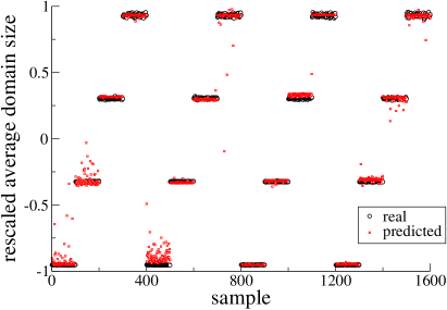
Figure 5: Real (circles) and predicted (squares) values of the rescaled average domain sizes for different samples (numbered $1$ to $1600$).

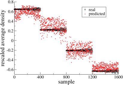
Figure 6: Real (circles) and predicted (squares) values of the rescaled average densities for different samples (numbered $1$ to $1600$).

Figures 5 and 6 show plots of the rescaled average domain size and rescaled average densities for each microstructure, along with the predictions output when the perceptron is trained with displacement DFA data from all remaining microstructures. Despite the relatively high average error (of $0.01$ for the domain sizes and $0.1$ for the densities), it is clear that the information hidden in the DFA vectors is enough to provide useful predictions for the unknown parameters. (Using data from pressure DFA vectors leads to a similar performance when predicting densities, but a five-fold increase in the average error when predicting domain sizes.) We also trained the perceptron to output both domain size and density, but the performance showed a considerable decline compared to the case when the parameters where targeted by different networks. An early-stopping criterion (see e.g. Ref. Haykin (1999)) was likewise implemented, but did not lead to improved results.

Finally, if the network is trained with a random selection of 1280 (80%) samples from all classes, the overall error in the testing stage is reduced to around $10^{-3}$ when targeting the average logarithmic domain size or average logarithmic density, indicating that this setup can also be used as a classifier, in the same spirit as the Gaussian discriminants of Sec. IV, although at a considerably higher computational cost.

VI Summary

Our aim in this work was to provide, within a controllable framework, a proof-of-principle for the identification of microstructures based on fluctuation analyses of ultrasound signals. With a slightly modified detrended-fluctuation analysis (DFA) algorithm, we were able to build an automated Gaussian classifier capable of assigning a DFA curve to the correct microstructure among 16 possibilities, corresponding to combinations of 4 average densities and 4 average domain sizes, with an error rate below 1%. Although not detailed here, an analogous classifier based on the original DFA algorithm of Ref. Peng et al. (1994), despite not providing a comparable performance (yielding a much larger error rate around 30%), is able to separate the microstructures according to their average densities with an error rate of about 2%. Incidentally, yet another analogous classifier based on Hurst’s $R/S$ analysis also performs modestly for overall classification, with an error rate of about 22%, but is able to separate the microstructures according to their average domain size with a success rate in excess of 99.7%.

We also described a multilayer perceptron which is able to provide estimates of a physical property for DFA curves from an unknown microstructure after being trained to output the corresponding property for the remaining microstructures.

The application of the methods described here to more realistic situations depends on a series of tests which incorporate effects coming from more complicated, higher-dimensional geometries. Among these effects, we mention mode conversion at domain interfaces and the presence of additional defects such as voids or inclusions of distinct phases. We hope the results reported in this paper will encourage future investigations.

Appendix A Solution of the wave equation for a one-dimensional heterogeneous medium

Figure 7: Sketch of the geometry used in simulating ultrasound propagation in an inhomogeneous medium. See main text for labels.

We want to solve the wave equation for the displacement field $\Phi\left(x,t\right)$,

$$\frac{\partial^{2}\Phi}{\partial x^{2}}=\frac{1}{c^{2}}\frac{\partial^{2}\Phi}{\partial t^{2}},$$ (18)

with the sound velocity $c$ a constant along each domain into which the one-dimensional system, of size $L$, is divided. This means that $\Phi\left(x,t\right)$ will be given by a different function in each domain, and the problem can be recast as the solution of the wave equations

$$\frac{\partial^{2}\Phi_{j}}{\partial x^{2}}=\frac{1}{c_{j}^{2}}\frac{\partial^{2}\Phi_{j}}{\partial t^{2}},$$ (19)

for every domain $j$, subject to the boundary conditions

$$\Phi_{j-1}\left(x_{j},t\right)=\Phi_{j}\left(x_{j},t\right)$$ (20)

and

$$\rho_{j-1}c_{j-1}^{2}\frac{\partial\Phi_{j-1}}{\partial x}\left(x_{j},t\right)=\rho_{j}c_{j}^{2}\frac{\partial\Phi_{j}}{\partial x}\left(x_{j},t\right),$$ (21)

describing the continuity of the displacement and the pressure fields at the interfaces between domains. Here, $c_{j}$ and $\rho_{j}$ denote the sound velocity and the density in domain $j$, while $x_{j}$ is the coordinate of the left end of domain $j$. The medium is divided into $N+2$ domains $\left(j\in\left\{-1,0,1,2,\ldots,N\right\}\right)$, with $x_{-1}=0$ and $x_{N+1}=L$; see Figure 7. Domains from $j=1$ to $j=N$ correspond to the medium to be investigated, and span a length $W<L$. Domain $j=0$ holds a piezoelectric transducer, in which the ultrasonic pulse is to be produced, and domain $j=-1$ is reserved for an “escape area”, introduced to mimic the presence of an absorbing wall at the back of the transducer.

Separation of variables leads to a general solution of Eq. (19), for a given angular frequency $\omega$, of the form

$$\Phi_{j}\left(x,t;\omega\right) = \left[A_{j}\cos\left(k_{j}x\right)+B_{j}\sin\left(k_{j}x\right)\right]\cos\left(\omega t\right)$$ (22)

$$+ \left[C_{j}\cos\left(k_{j}x\right)+D_{j}\sin\left(k_{j}x\right)\right]\sin\left(\omega t\right).$$

Since we will impose initial conditions in which $\frac{\partial\Phi_{j}}{\partial t}\equiv 0$, we can set $C_{j}=D_{j}=0$ for all $j$. The boundary conditions in Eq. (20) and (21) lead to

$$\frac{A_{j-1}\cos\left(k_{j-1}x_{j}\right)+B{}_{j-1}\sin\left(k_{j-1}x_{j}\right)}{A_{j}\cos\left(k_{j}x_{j}\right)+B{}_{j}\sin\left(k_{j}x_{j}\right)}=1$$ (23)

and

$$\frac{z_{j-1}\left[A_{j-1}\sin\left(k_{j-1}x_{j}\right)-B{}_{j-1}\cos\left(k_{j-1}x_{j}\right)\right]}{z_{j}\left[A_{j}\sin\left(k_{j}x_{j}\right)-B{}_{j}\cos\left(k_{j}x_{j}\right)\right]}=1$$ (24)

for $j\in\left\{0,1,2,\ldots,N\right\},$ in which we introduced the acoustic impedances $z_{j}=\rho_{j}c_{j}$, while the reflective boundary conditions at $x=0$ and $x=L$, $\Phi_{-1}\left(0,t\right)=\Phi_{N}\left(L,t\right)=0$, yield

$$\left\{\begin{array}[]{l}A_{-1}=0,\\ A_{N}\cos\left(k_{N}L\right)+B_{N}\sin\left(k_{N}L\right)=0.\end{array}\right.$$ (25)

In order to mimic an absorbing wall at the back of the transducer (at $x=x_{0}$), we choose for domain $j=-1$ an acoustic impedance $z_{-1}=z_{0}$ and a very small sound velocity $c_{-1}$. These choices guarantee that waves incident on the left end of the transducer are not reflected, rather entering the escape area and not returning during the simulation.

Equations (23), (24) and (25) constitute a homogeneous system of linear equations in the coefficients $A_{j}$ and $B_{j}$. Rewriting the system as the matrix equation

$$\left(\begin{array}[]{ccccccc}A_{-1}&B_{-1}&A_{0}&B_{0}&\cdots&A_{N}&B_{N}\end{array}\right)\mathbf{M}_{N}=0,$$ (26)

in which

$$\mathbf{M}_{N}=\left[\begin{array}[]{ccccccccc}1&\cos\left(k_{-1}x_{1}\right)&z_{-1}\sin\left(k_{-1}x_{1}\right)&0&0&\cdots&0&0&0\\ 0&\sin\left(k_{-1}x_{1}\right)&-z_{-1}\cos\left(k_{-1}x_{1}\right)&0&0&\cdots&0&0&0\\ 0&-\cos\left(k_{0}x_{1}\right)&-z_{0}\sin\left(k_{0}x_{1}\right)&\cos\left(k_{0}x_{1}\right)&z_{0}\sin\left(k_{0}x_{1}\right)&\cdots&0&0&0\\ 0&-\sin\left(k_{0}x_{1}\right)&z_{0}\cos\left(k_{0}x_{1}\right)&\sin\left(k_{0}x_{1}\right)&-z_{0}\cos\left(k_{0}x_{1}\right)&\cdots&0&0&0\\ 0&0&0&-\cos\left(k_{1}x_{1}\right)&-z_{1}\sin\left(k_{1}x_{1}\right)&\cdots&0&0&0\\ 0&0&0&-\sin\left(k_{1}x_{1}\right)&z_{1}\cos\left(k_{1}x_{1}\right)&\cdots&0&0&0\\ \vdots&\vdots&\vdots&\vdots&\vdots&\ddots&\vdots&\vdots&\vdots\\ 0&0&0&0&0&\cdots&\cos\left(k_{N-1}x_{N}\right)&z_{N-1}\sin\left(k_{N-1}x_{N}\right)&0\\ 0&0&0&0&0&\cdots&\sin\left(k_{N-1}x_{N}\right)&-z_{N-1}\cos\left(k_{N-1}x_{N}\right)&0\\ 0&0&0&0&0&\cdots&-\cos\left(k_{N}x_{N}\right)&-z_{N}\sin\left(k_{N}x_{N}\right)&\cos\left(k_{N}L\right)\\ 0&0&0&0&0&\cdots&-\sin\left(k_{N}x_{N}\right)&z_{N}\cos\left(k_{N}x_{N}\right)&\sin\left(k_{N}L\right)\end{array}\right],$$ (27)

we see that nontrivial solutions for the $\left\{A_{j},B_{j}\right\}$ are obtained only if

$$\det\mathbf{M}_{N}=0,$$

an equation whose solutions correspond to the eigenfrequencies $\omega_{k}$. Minor-expanding the determinant using the last column of $\mathbf{M}_{N}$ leads to the recursion formulas

$$m_{n}\equiv\det\mathbf{M}_{n}=-\cos\left(k_{n}x_{n+1}\right)f_{n}+\sin\left(k_{n}x_{n+1}\right)g_{n},$$ (28)

with

$$\left\{\begin{array}[]{ccc}f_{n}&=&\sin\left(k_{n}x_{n}\right)h_{n-1}+z_{n}\cos\left(k_{n}x_{n}\right)m_{n-1},\\ g_{n}&=&\cos\left(k_{n}x_{n}\right)h_{n-1}-z_{n}\sin\left(k_{n}x_{n}\right)m_{n-1},\\ h_{n}&=&-z_{n}\sin\left(k_{n}x_{n+1}\right)f_{n}-z_{n}\cos\left(k_{n}x_{n+1}\right)g_{n},\end{array}\right.$$ (29)

subject to the initial conditions

$$m_{-1}=\sin\left(k_{-1}x_{0}\right)\qquad\mbox{and}\qquad h_{-1}=-z_{-1}\cos\left(k_{-1}x_{0}\right).$$

These formulas allow the numerical evaluation of the determinant for an arbitrary value of $\omega$. For a given geometry, the eigenfrequencies are numerically determined by first sweeping through the values of $\omega$, with a certain increment $\delta\omega$, until $\det\mathbf{M}_{N}$ changes sign, bracketing an eigenfrequency whose value is then refined by the bisection method. The process is repeated with decreasing values of $\delta\omega$ until no additional eigenfrequencies up to a previously set value $\omega_{\mathrm{max}}$ are found. For a given eigenfrequency $\omega_{k}$, the corresponding coefficients $\left\{A_{jk},B_{jk}\right\}$ (with a new index $k$ to indicate the dependence on $\omega_{k}$) are determined recursively from Eqs. (23) and (25), supplemented by the normalization condition $B_{-1,k}=1.$

The general solution of the full wave equation then takes the form

$$\Phi\left(x,t\right)=\sum_{k}\phi_{k}X_{k}\left(x\right)\cos\left(\omega_{k}t\right),$$ (30)

in which

$$X_{k}\left(x\right)=A_{jk}\cos\left(\omega_{k}x/c_{j}\right)+B_{jk}\sin\left(\omega_{k}x/c_{j}\right),$$ (31)

with $j$ such that $x_{j}\leq x<x_{j+1}$. The constant coefficients $\phi_{k}$ are derived from the initial condition $\Phi\left(x,0\right)$ by using the orthogonality condition satisfied by the $X_{k}\left(x\right)$,

$$\sum_{j=-1}^{N}\rho_{j}\int_{x_{j}}^{x_{j+1}}dxX_{k}\left(x\right)X_{q}\left(x\right)=\xi_{k}\delta_{kq}.$$ (32)

Explicitly, we have

$$\phi_{k}=\frac{1}{\xi_{k}}\sum_{j=-1}^{N}\rho_{j}\int_{x_{j}}^{x_{j+1}}dx\Phi\left(x,0\right)X_{k}\left(x\right),$$ (33)

with $\xi_{k}>0$ defined by Eq. (32). The conclusion that the orthogonality condition involves the densities $\rho_{j}$ comes from integrating, over the entire system, the differential equation satisfied by $X_{k}\left(x\right)$, multiplied by $X_{q}\left(x\right)$, then exchanging the roles of $q$ and $k$, and subtracting the results, taking into account the continuity of the pressure at the interfaces. The above orthogonality condition follows if $\omega_{k}\neq\omega_{q}$.

References

- Anderson (1958) P. W. Anderson, Phys. Rev. 109, 1492 (1958).
- Hodges (1982) C. H. Hodges, Journal of Sound and Vibration 82, 411 (1982).
- Baluni and Willemsen (1985) V. Baluni and J. Willemsen, Phys. Rev. A 31, 3358 (1985).
- Gavish and Castin (2005) U. Gavish and Y. Castin, Phys. Rev. Lett. 95, 020401 (2005).
- Bahraminasab et al. (2007) A. Bahraminasab, S. M. V. Allaei, F. Shahbazi, M. Sahimi, M. D. Niry, and M. R. R. Tabar, Phys. Rev. B 75, 064301 (2007).
- Hurst (1951) H. E. Hurst, Trans. Am. Soc. Civ. Eng. 116, 770 (1951).
- Matos et al. (2004) J. M. O. Matos, E. P. de Moura, S. E. Krüger, and J. M. A. Rebello, Chaos, Solitons & Fractals 19, 55 (2004).
- Peng et al. (1994) C. K. Peng, S. V. Buldyrev, S. Havlin, M. Simons, H. E. Stanley, and A. L. Goldberger, Phys. Rev. E 49, 1685 (1994).
- Ossadnik et al. (1994) S. M. Ossadnik, S. V. Buldyrev, A. L. Goldberger, S. Havlin, R. N. Mantegna, C. K. Peng, M. Simons, and H. E. Stanley, Biophysical Journal 67, 64 (1994).
- Goldberger et al. (2002) A. L. Goldberger, L. A. N. Amaral, J. M. Hausdorff, P. C. Ivanov, C.-K. Peng, and H. E. Stanley, Proceedings of the National Academy of Sciences of the United States of America 99, 2466 (2002).
- Hausdorff et al. (2000) J. M. Hausdorff, A. Lertratanakul, M. E. Cudkowicz, A. L. Peterson, D. Kaliton, and A. L. Goldberger, Journal of Applied Physiology 88, 2045 (2000).
- Hwa and Ferree (2002) R. C. Hwa and T. C. Ferree, Phys. Rev. E 66, 021901 (2002).
- Peng et al. (2002) C. K. Peng, J. E. Mietus, Y. H. Liu, C. Lee, J. M. Hausdorff, H. E. Stanley, A. L. Goldberger, and L. A. Lipsitz, Ann. Biomed. Eng. 30, 683 (2002).
- Fraedrich and Blender (2003) K. Fraedrich and R. Blender, Phys. Rev. Lett. 90, 108501 (2003).
- Webb (2002) A. R. Webb, Statistical Pattern Recognition, 2nd ed. (John Wiley & Sons, West Sussex, 2002).
- Vieira et al. (2008) A. P. Vieira, E. P. de Moura, L. L. Gonçalves, and J. M. A. Rebello, Chaos, Solitons & Fractals 38, 748 (2008).
- Vieira et al. (2009) A. P. Vieira, H. H. M. Vasconcelos, L. L. Gonçalves, and H. C. de Miranda, in Review of Progress in Quantitative Nondestructive Evaluation (2009), vol. 1096 of AIP Conference Proceedings, pp. 564–571.
- de Moura et al. (2009) E. P. de Moura, A. P. Vieira, M. A. Irmão, and A. A. Silva, Mech. Syst. Signal Process. 23, 682 (2009).
- Vieira et al. (2010) A. P. Vieira, E. P. de Moura, and L. L. Gonçalves, EURASIP Journal on Advances in Signal Processing 2010, 262869 (2010).
- Podobnik and Stanley (2008) B. Podobnik and H. E. Stanley, Phys. Rev. Lett. 100, 084102 (2008).
- Addison (1997) P. S. Addison, Fractals and Chaos (IOP, London, 1997).
- Ovchinnikov et al. (2009) O. S. Ovchinnikov, S. Jesse, P. Bintacchit, S. Trolier-McKinstry, and S. V. Kalinin, Phys. Rev. Lett. 103, 157203 (2009).
- Kumar et al. (2011) A. Kumar, O. Ovchinnikov, S. Guo, F. Griggio, S. Jesse, S. Trolier-McKinstry, and S. V. Kalinin, Phys. Rev. B 84, 024203 (2011).
- Rumelhart et al. (1986) D. Rumelhart, G. Hinton, and R. Williams, in Parallel Distributed Processing: Explorations in the Microstructure of Cognition, edited by D. Rumelhart, J. McClelland, and the PDP Research Group (MIT Press, 1986), vol. 1, pp. 318–362.
- Duda et al. (2000) R. O. Duda, P. E. Hart, and D. G. Stork, Pattern Classification, 2nd ed. (Wiley Interscience, New York, 2000).
- Haykin (1999) S. Haykin, Neural Networks: A Comprehensive Foundation, 2nd ed. (Prentice Hall, 1999).