Accretion Properties of High- and Low-Excitation Young Radio Galaxies

Abstract

Young radio galaxies (YRGs) provide an ideal laboratory to explore the connection between accretion disk and radio jet thanks to their recent jet formation. We investigate the relationship between the emission-line properties, the black hole accretion rate, and the radio properties using a sample of 34 low-redshift ($z<0.4$) YRGs. We classify YRGs as high-excitation galaxies (HEGs) and low-excitation galaxies (LEGs) based on the flux ratio of high-ionization to low-ionization emission lines. Using the H$\alpha$ luminosities as a proxy of accretion rate, we find that HEGs in YRGs have $\sim 1$ dex higher Eddington ratios than LEGs in YRGs, suggesting that HEGs have higher mass accretion rate or higher radiative efficiency than LEGs. In agreement with previous studies, we find that the luminosities of emission lines, in particular H$\alpha$, are correlated with radio core luminosity, suggesting that accretion and young radio activities are fundamentally connected.

1. INTRODUCTION

Active galactic nuclei (AGN) play an important role in galaxy evolution by feeding their host galaxies with radiative and/or kinetic energy, leading to the observed scaling relations between black hole (BH) mass and galaxy properties (e.g., Ferrarese & Merritt 2000; Gültekin et al. 2009; Woo et al. 2010). Thus, investigating the radiative and kinetic processes of AGN is of fundamental importance for understanding AGN physics as well as feedback mechanisms.

The formation of relativistic jets and its connection to accretion disk remain as an open issue in AGN physics (e.g., Rees 1984; Meier 2003; McKinney 2006; Komissarov et al. 2007; McKinney et al. 2012). Thanks to their short dynamical timescale, X-ray binaries in various states have been observed in detail, revealing that individual sources occupy a particular accretion state with various X-ray and radio luminosities (e.g., Fender et al. 2004; Remillard & McClintock 2006). By analogy to X-ray binaries, the power of AGN jets may also depend on the physical states of accretion disk.

However, the disk-jet connection is more complicated in AGNs. It has been known that the radio power is correlated with narrow emission line luminosities, i.e., [O iii], which is a proxy for the accretion power (e.g., Baum & Heckman 1989; Rawlings & Saunders 1991), indicating that the jet launching mechanism is connected with accretion disk. However, the correlation shows a large scatter (e.g., Morganti et al. 1992; Labiano 2008), implying that the nature of the disk-jet connection is complicated and that other physical parameters are necessary to constrain.

The properties of the accretion disk seem to play an additional role in the disk-jet connection. At a given radio luminosity, high-excitation galaxies (HEG) classified with high [O iii]/H$\alpha$ ratio (e.g., Laing et al. 1994) have an order of magnitude higher [O iii] luminosity than low-excitation galaxies (LEG). Using a sample of 3C radio galaxies, Buttiglione et al. (2010) showed that there are two sequences in the radio–emission line luminosity plane, suggesting that systematically different accretion rates or accretion modes are responsible for the separation between HEGs and LEGs.

One of the limiting factors in interpreting the disk-jet connection in powerful radio galaxies is that the lifetime of large radio sources is much longer than the transition timescale of the physical states in the accretion disk (O’Dea et al. 2009). Thus, comparing radio and accretion powers in radio galaxies with large-scale jets may suffer systematic uncertainties, leading to large scatters in the correlation between optical and radio properties (see Punsly & Zhang 2011).

In contrast, compact radio galaxies with small jets triggered by recent activity are very useful to investigate the disk-jet connection, since radio and disk activities are contemporaneous. The ages of compact radio galaxies are typically estimated as $t_{\rm age}=10^{2}-10^{3}$ years (e.g., Orienti et al. 2007; Fanti 2009; Giroletti & Polatidis 2009), while the lifetime of extended (up to a few hundred kpc) radio sources are about $10^{6}-10^{7}$ years (e.g., Alexander & Leahy 1987; Carilli et al. 1991; Fanti et al. 1995; O’Dea et al. 2009).

Recently, a substantial amount of such compact radio galaxies have been detected and classified with various characteristics: compact symmetric objects (CSO) with a linear scale $\lesssim 1$ kpc, gigahertz-peaked spectrum (GPS; $\lesssim 1$ kpc) sources, medium-size symmetric objects ($1-10$ kpc), and compact steep-spectrum (CSS; $\lesssim 20$ kpc) sources (See O’Dea et al. 2009). These young radio galaxies (YRGs) are a good laboratory to investigate the physical link between AGN jets and accretion disks.

YRGs show a close connection between emission-line gas and radio properties. For example, it has been reported that emission-line gas (e.g.,[O ii], [O iii]) is well aligned with the radio jet (e.g., de Vries et al. 1999; Axon et al. 2000) and that emission-line luminosities (e.g., [O iii]) are correlated with the radio power (e.g., Labiano 2008; Buttiglione et al. 2010; Kunert-Bajaraszewska & Labiano 2010). The optical emission-line diagnostics of the narrow-line region (NLR) can constrain accretion properties, since the NLR is photoionized by the nuclear continuum radiation (e.g., Kawakatu et al. 2009).

In this work, using a sample of YRGs covering a large range of luminosities, we investigate the properties of NLRs and accretion by directly measuring narrow emission-line luminosities from optical spectra, and compare them with radio properties for constraining the disk-jet connection. In Section 2, we describe the sample selection, spectroscopic observations, data reduction, and radio data collection. The measurements of emission-line fluxes and the stellar velocity dispersions are described in Section 3. Main results are presented in Section 4 and Section 5 contains discussions and summary. Throughout the paper, we used cosmological parameters, $H_{0}=70$ km s^-1  Mpc^-1, $\Omega_{m}=0.3$, and $\Omega_{\Lambda}=0.7$.

Table 1Sample properties

Name	R.A.	Decl.	z	$E(B-V)$	AGN type			$S_{1.4}$	Ref.	Jet size	Ref.	Run	Exposure	S/N
	(J2000)							(Jy)		(kpc)			(hr)
(1)	(2)	(3)	(4)	(5)	(6)	(7)	(8)	(9)	(10)	(11)	(12)	(13)	(14)	(15)
Lick and Palomar targets
0019$-$000	00:22:25	+00:14:56	0.305	0.027	2	GPS	HEG	2.919	F	0.121	O98	1	1.4	48
0035+227	00:38:08	+23:03:28	0.096	0.033	2	CSO	LEG	0.547	N	0.015	K08	3	2	73
0134+329	01:37:41	+33:09:35	0.367	0.044	1	CSS	HEG	16.018	N	1.100	O98	4	1	208
0221+276	02:24:12	+27:50:12	0.310	0.125	1	CSS	HEG	3.024	N	5.536	K08	4	1.5	32
0316+413	03:19:48	+41:30:42	0.018	0.163	1	CSO	HEG	22.829	N	0.005	K08	3	1	169
0345+337	03:48:47	+33:53:15	0.243	0.389	2	CSS	LEG	2.365	N	0.443	O98	5	3	11
0428+205	04:31:04	+20:37:34	0.219	0.542	2	GPS	LEG	3.756	N	0.412	O98	2	1.5	16
0605+480	06:09:33	+48:04:15	0.277	0.162	2	CSS	LEG	4.133	N	15.17	K08	5	3	12
0941$-$080	09:43:37	$-$08:19:31	0.228	0.029	2	GPS	LEG	2.756	N	0.083	O98	6	1.5	10
1203+645	12:06:25	+64:13:37	0.372	0.017	1	CSS	HEG	3.719	N	3.067	K08	10	3	21
1225+442	12:27:42	+44:00:42	0.348	0.019	2	GPS	HEG	0.383	F	0.493	K08	7	1.5	9
1233+418	12:35:36	+41:37:07	0.250	0.022	2	CSS	LEG	0.664	F	6.068	K10	7	0.5	8
1245+676	12:47:33	+67:23:16	0.107	0.021	2	CSO	LEG	0.263	N	0.007	K08	7	1.5	141
1250+568	12:52:26	+56:34:20	0.320	0.010	1	CSS	HEG	2.442	F	3.593	K08	8	1.5	67
1323+321	13:26:17	+31:54:10	0.368	0.015	2	GPS	HEG	4.747	F	0.149	K08	10	1.5	34
1404+286	14:07:00	+28:27:15	0.077	0.018	1	GPS	HEG	0.830	F	0.005	K08	9	1	53
1807+698	18:06:51	+69:49:28	0.051	0.036	2	CSS	LEG	1.886	N	1.726	G94	3	1.5	120
1943+546	19:44:32	+54:48:07	0.263	0.162	2	CSO	$\cdots$	1.754	N	0.072	K08	2	1.5	13
2352+495	23:55:09	+49:50:08	0.238	0.181	2	GPS	LEG	2.306	N	0.092	K08	2	2	21
SDSS targets
0025+006	00:28:33	+00:55:11	0.104	0.024	2	CSS	HEG	0.237	F	2.230	K10		$\cdots$	21
0754+401	07:57:57	+39:59:36	0.066	0.054	2	CSS	HEG	0.099	F	0.178	K10		$\cdots$	28
0810+077	08:13:24	+07:34:06	0.112	0.022	2	CSS	LEG	0.463	F	1.982	K10		$\cdots$	19
0921+143	09:24:05	+14:10:22	0.136	0.029	2	CSS	LEG	0.108	F	0.520	K10		$\cdots$	19
0931+033	09:34:31	+03:05:45	0.225	0.033	2	CSS	LEG	0.292	F	1.140	K10		$\cdots$	22
0942+355	09:45:26	+35:21:03	0.208	0.011	1	CSS	HEG	0.148	F	3.138	K10		$\cdots$	20
1007+142	10:09:56	+14:01:54	0.213	0.043	2	CSS	LEG	1.045	F	2.320	K10		$\cdots$	18
1037+302	10:40:30	+29:57:58	0.091	0.019	2	CSS	LEG	0.388	F	2.591	K10		$\cdots$	30
1154+435	11:57:28	+43:18:06	0.230	0.013	1	CSS	HEG	0.256	F	3.227	K10		$\cdots$	21
1345+125	13:47:33	+12:17:24	0.122	0.034	1	GPS	HEG	4.860	F	0.085	O98		$\cdots$	17
1407+363	14:09:42	+36:04:16	0.148	0.012	2	CSS	HEG	0.143	F	0.050	K10		$\cdots$	9
1521+324	15:23:49	+32:13:50	0.110	0.026	2	CSS	HEG	0.169	F	0.285	K10		$\cdots$	17
1558+536	15:59:28	+53:30:55	0.179	0.012	2	CSS	LEG	0.182	F	3.630	K10		$\cdots$	17
1601+528	16:02:46	+52:43:58	0.106	0.019	1	CSS	LEG	0.576	F	0.269	K10		$\cdots$	26
1610+407	16:11:49	+40:40:21	0.151	0.008	2	CSS	LEG	0.553	F	1.858	K10		$\cdots$	12

Note. — Columns: (1) Target name; (2) R.A.; (3) Decl..; (4) Redshift; (5) Galactic extinction; (6) Spectroscopic AGN type – 1: Type 1 AGN with broad emission lines; 2: Type 2 AGN without broad emission line; (7) YRG type; (8) Classification by excitation – HEG: high excitation galaxy, LEG: low excitation galaxy; (9) 1.4 GHz integrated flux density of radio source; (10) Reference for the flux density – F: from the Faint Images of the Radio Sky at Twenty-centimeters (FIRST) catalog, N: from the NRAO/VLA Sky Survey (NVSS) catalog; (11) Jet size; (12) Reference for the jet size – G94: Gelderman & Whittle (1994), O98: O’Dea (1998), K08: Kawakatu et al. (2008); K10: Kunert-Bajaraszewska et al. (2010); (13) Observing run in Table 2; (14) Exposure time; (15) Signal-to-noise ratios near 5100 Å in the rest frames.

2. OBSERVATIONS AND DATA

2.1. Sample Selection

To investigate the properties of optical emission lines and their connection to radio activities, we selected a sample of 34 YRGs from the literature. Initially, we selected 19 known YRGs listed by O’Dea (1998) and Kawakatu et al. (2008), by limiting a redshift range $z<0.4$. This choice was made in order to include narrow emission lines from [O II] to [Ar III] ($3727-7136$ Å in the rest-frame) in the observed wavelength range for comparing emission-line flux ratios with the photoionization models.

During our observing campaign, new YRGs with relatively low luminosity have been reported by Kunert-Bajaraszewska et al. (2010) based on the unresolved and isolated morphology in Faint Images of the Radio Sky at Twenty-centimeters (FIRST). To enlarge the sample size and the luminosity range, we selected additional 15 YRGs at $z<0.3$ from their list, for which optical spectra with the same rest-frame wavelength range ($3727-7136$ Å) were available in the archive of the Sloan Digital Sky Survey (SDSS) Data Release 7 (DR7; Abazajian et al. 2009). Thus, combining new data with SDSS archival data, we compiled a sample of 34 low-redshift YRGs for investigating optical and radio properties. Table 1 lists the properties of individual YRGs, including optical and radio AGN classifications.

2.2. New Optical Data

Among 34 objects in the sample, SDSS spectra are available for 15 objects, while for the remaining 19 objects, new spectroscopic data have been obtained from the Lick and Palomar telescopes. In this section, we describe new observations and data reduction.

2.2.1 Observations

We observed 19 YRGs to obtain high-quality optical spectra. Ten objects were observed with the Kast double spectrograph at the Lick 3 m telescope (Miller & Stone 1993). We used the D55 dichroic beam splitter to pass the light into blue and red side detecters. Depending on the redshift of the target, different gratings were used in the red spectrograph, covering the wavelength range of $5500-10000$ Å  with a wavelength scale of $1.7-4.6$ Å pixel^-1 and spatial scale of $0.78$ arcsec pixel^-1. For the blue spectrograph, the 600/4310 grism was used, covering the wavelength range $3600-5500$ Å with a wavelength scale of $1.0$ Å pixel^-1 and spatial scale of $0.43$ arcsec pixel^-1.

The other nine galaxies were observed withthe Double Spectrograph for the Palomar 200-inch Telescope (DBSP; Oke & Gunn 1982) using the D55 or D68 dichroic mirrors depending on the redshift of the targets. The 158/7500 and 316/7500 gratings were used on the red spectrograph, covering $5200-10000$ Å with a wavelength scale of 4.8 or 2.4 Å pixel^-1 and spatial scale of $0.62$ arcsec pixel^-1, while the 600/4000 grating was used on the blue spectrograph, covering the wavelength range of $3200-5500$ Å or $4000-6800$ Å with a wavelength scale of $\sim 1.1$ Å pixel^-1 and spatial scale of $0.39$ arcsec pixel^-1.

For all observations, a 2″-wide slit was centered on the nucleus of the targets after aligned with a parallactic angle. Several flux photometric standard stars, namely, BD+262606, BD+284211, Feige 34, G138-31, G191B2B, HD192281, or Wolf1346 were observed during each night. A0V stars with similar airmass and hour angle to each target were observed for telluric correction. The properties of each YRG along with exposure time and S/N are presented in Table 1, while the details of instrumental setup, observing date, and sky conditions are listed in Table 2 .

Figure 1.— Reduced spectra of 19 YRGs obtained with the Kast at the Lick telescope or the DBSP at the Palomar telescope.

Figure 2.— Spectra of 15 additional YRGs obtained from the SDSS DR7.

2.2.2 Data Reduction

Standard spectroscopic data reduction procedures, including bias subtraction, flat-fielding, spectral extraction, wavelength calibration, and flux calibration, were carried out for each data set using a series of IRAF scripts developed for long-slit data (e.g., Woo et al. 2005, 2006). Telluric A and B bands were corrected using an A0V star spectrum obtained for each target as similarly performed in the previous studies (e.g., Woo et al. 2006). After combining multiple exposures in each blue and red sides, the blue- and red-side spectra were merged into one final spectrum for each target. Galactic extinction corrections were applied using the extinction law by Cardelli et al. (1989) with the $E(\bv)$ values listed in Table 1. We measured the spectral resolution by averaging the width of sky or arc lines for each instrumental setup (see Table 2). In the case of the SDSS archival data, the spectra were obtained with a 3″ diameter fiber and a spectral resolution of $\lambda/\Delta\lambda\approx 1800$.

2.3. Radio Data

To compare with optical spectroscopic properties, we collected the radio luminosity and the jet size of the sample from the literature, after correcting for the adopted cosmological parameters. The 1.4 GHz integrated flux densities of radio core were extracted from the FIRST catalog, while the NRAO/VLA Sky Survey (NVSS) catalog was used if FIRST data were not available. We confirmed that these integrated flux densities were measured from radio core by checking the presence of unresolved radio cores in the FIRST and NVSS images. The integrated flux densities and their references are listed in Table 1.

The jet size is generally defined by a half of the linear scale or the hot spot distance from the core. We collected the linear jet sizes from the literature after correcting for the adopted cosmological parameters. The radio luminosity and the jet size of each object are listed in Table 1.

3. ANALYSIS

In this section, we present AGN emission and stellar absorption line measurements based on the optical spectra. First, we describe AGN classification based on the presence of the broad H$\alpha$ line in Section 3.1. Second, we present the emission-line fitting procedure and measurements in Section 3.2. Then, we describe the stellar velocity dispersion measurements in Section 3.3.

3.1. The Spectra

In Figure 1, we present the spectra of 19 YRGs obtained from the Lick and Palomar telescopes. For completeness, we also present SDSS spectra of 15 additional YRGs in Figure 2. We classified YRG as Type 1 and Type 2 based on the presence of the broad H$\alpha$ line. The sample is composed of 10 Type 1 (i.e., broad-line) and 24 Type 2 (i.e., narrow-line) AGNs as listed in Table 1. For Type 1 objects, the broad H$\alpha$ component was clearly present although the broad H$\beta$ were not detected for three objects, presumably due to the weak flux level of the broad H$\beta$ component (for details, see Figure 3). In Type 2 objects, stellar absorption lines were dominant as expected, confirming that subtracting stellar absorption lines is important to precisely measure AGN emission line fluxes. While one object 0810+077 was previously classified as Type 1 AGN, the broad H$\alpha$ was not detected in our spectra, hence we classified it as a Type 2 AGN.

The optical spectra of 0428+205, 1203+645, 1225+442, 1233+418, and 1323+321 are newly presented in this paper. The spectra of other objects have higher spectral resolution and/or better S/N than spectra presented by previous studies (e.g., Gelderman & Whittle 1994: 0134+329, 0221+276, 0345+337, and 1250+568; Labiano et al. 2005 and O’Dea et al. 2002: 0221+276 and 1250+568; Buttiglione et al. 2009: 0345+337, 0605+480, and 1807+698).

Table 2Journal of observations

Run	Date	Tel.	Inst.	Dichr.	Blue side				Red side				Seeing	Sky
					Grism	Plate	Spatial	Res.	Grating	Plate	Spatial	Res.
					(l mm-1)	(Å pixel-1)	(arcsec pixel-1)	(Å)	(l mm-1)	(Å pixel-1)	(arcsec pixel-1)	(Å)	(arcsec)
(1)	(2)	(3)	(4)	(5)	(6)	(7)	(8)	(9)	(10)	(11)	(12)	(13)	(14)	(15)
1	2009 Jul 21	P	D	D55	600	1.1	0.39	5.0	158	4.8	0.62	16.3	$\sim$2	clear
2	2009 Aug 23	P	D	D68	600	1.1	0.39	5.0	316	2.4	0.62	8.1	$\sim$2.2	clear
3	2009 Aug 23	L	K	D55	600	1.0	0.43	4.4	600	2.4	0.78	6.1	$\sim$1.3	clear
4	2009 Aug 24	L	K	D55	600	1.0	0.43	4.4	300	4.6	0.78	13.0	$\sim$1.5	clear
5	2009 Dec 09	P	D	D68	600	1.1	0.39	5.0	316	2.4	0.62	8.1	$\sim$2	thick
6	2009 Dec 16	L	K	D55	600	1.0	0.43	4.4	300	4.6	0.78	13.0	$\sim$1.5	thin
7	2010 Jan 14	P	D	D68	600	1.1	0.39	5.0	316	2.4	0.62	8.1	$\sim$3	thin
8	2010 Mar 10	L	K	D55	600	1.0	0.43	4.4	300	4.6	0.78	13.0	$\sim$1.5	humid
9	2011 Jan 06	L	K	D55	600	1.0	0.43	4.4	830	1.7	0.78	4.2	$\sim$1.5	clear
10	2011 Jan 07	L	K	D55	600	1.0	0.43	4.4	300	4.6	0.78	13.0	$\sim$2	clear

Note. — Columns: (1) Observing run; (2) Observation date (UT); (3) Telescope (P: Palomar 5 m, L: Lick 3 m); (4) Spectrograph (D: DBSP, K: Kast); (5) Dichroic mirrors; (6) & (10) Grism for the blue side and Grating for the red side, respectively; (7) & (11) Plate scales for the blue and red sides, respectively; (8) & (12) Spatial scales for the blue and red sides, respectively; (9) & (13) Instrumental resolution; (14) Seeing; (15) Sky condition.

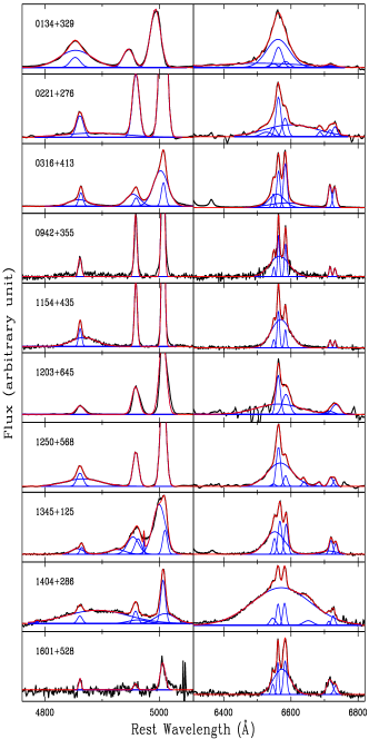
Figure 3.— H$\beta$ and H$\alpha$ regions of Type 1 AGNs. Broad and narrow components of H$\beta$ and H$\alpha$ lines and narrow forbidden lines, i.e., [O iii], [N ii] and [S ii] in the continuum-subtracted spectra (black lines) were simultaneously fitted with Gaussian models (blue). The combined fit is represented by red lines. (A color version of this figure is available in the online journal.)

Figure 4.— H$\beta$ and H$\alpha$ regions of Type 2 AGNs. Narrow H$\beta$ and H$\alpha$ lines, and [O iii], [N ii] and [S ii] in the continuum-subtracted spectra (black lines) were simultaneously fitted with Gaussian models (blue). The combined fit is represented by red lines. (A color version of this figure is available in the online journal.)

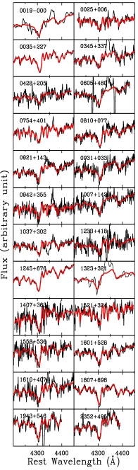
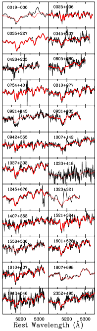
Figure 5.— Stellar velocity dispersion fitting in the G band (4300 Å) (left), Mg $b$ triplet region (right). The observed spectra (black lines) were compared with the best stellar template models (red lines). When the quality of the fit is poor (thin dashed lines), the measurements are discarded. Note that non-stellar lines, e.g., H$\gamma$, [O iii]$\lambda$4363, and [N i]$\lambda$5200 lines were masked out before the fitting procedure. (A color version of this figure is available in the online journal.)

Table 3Narrow emission-line fluxes for the line diagnostics

Name	[O ii]	[Ne iii]	[O iii]	H$\beta$	[O iii]	[O iii]	[O i]	H$\alpha$	[N ii]	[S ii]	[S ii]	[Ar iii]	E.I.
	3727	3869	4363	4861	4959	5007	6300	6563	6583	6716	6731	7136
(1)	(2)	(3)	(4)	(5)	(6)	(7)	(8)	(9)	(10)	(11)	(12)	(13)	(14)
0019$-$000	4.7	0.9	$\cdots$	0.8	0.8	6.6	$\cdots$	6.0	6.5	3.8	1.4	$\cdots$	$\cdots$
0025+006	159.7	25.2	$\cdots$	19.6	47.1	143.3	25.8	96.9	151.9	57.6	47.4	1.8	0.98
0035+227	110.8	$\cdots$	$\cdots$	14.0	$\cdots$	51.4	$\cdots$	66.0	50.8	$\cdots$	$\cdots$	$\cdots$	$\cdots$
0134+329	100.4	72.8	$\cdots$	104.2	198.2	615.2	28.2	372.9	110.7	43.2${\dagger}$		$\cdots$	1.63
0221+276	33.9	11.8	5.4	15.9	44.4	131.7	9.0	51.8	26.7	8.7	12.8	$\cdots$	1.39
0316+413	3395.6	1201.0	$\cdots$	682.2	2467.0	7594.1	3074.4	3377.9	4160.5	1894.2	1988.2	65.1	1.01
0345+337	140.9	21.8	$\cdots$	26.2	58.4	178.4	27.2	83.9	140.1	60.0	38.1	5.5	0.90
0428+205	25.0	$\cdots$	$\cdots$	3.4	6.3	20.5	26.6	39.4	53.5	18.4	19.4	$\cdots$	0.80
0605+480	53.0	6.3	$\cdots$	8.0	11.2	34.7	10.7	34.0	38.1	18.1	14.4	$\cdots$	0.79
0754+401	76.3	20.7	2.1	20.9	61.8	187.7	14.1	108.2	98.8	34.6	29.5	4.7	1.34
0810+077	67.1	6.0	$\cdots$	12.2	9.5	27.8	22.7	68.9	118.5	48.6	44.5	$\cdots$	0.40
0921+143	79.0	5.2	$\cdots$	13.9	4.6	13.1	26.0	41.7	96.5	35.5	44.0	$\cdots$	-0.17
0931+033	30.2	3.2	$\cdots$	4.5	4.4	16.3	7.0	27.1	34.6	14.3	14.8	$\cdots$	0.71
0941$-$080	18.8	3.1	$\cdots$	4.3	4.5	15.2	4.6	12.2	11.8	4.7	6.3	6.0	0.71
0942+355	22.3	13.6	$\cdots$	11.0	31.1	93.3	$\cdots$	22.6	21.5	6.4	5.6	$\cdots$	$\cdots$
1007+142	31.0	$\cdots$	$\cdots$	4.8	2.6	7.3	7.7	13.5	35.8	12.7	12.7	$\cdots$	0.03
1037+302	72.4	14.6	$\cdots$	3.0	5.8	26.3	17.7	53.4	133.2	42.8	31.0	$\cdots$	0.92
1154+435	37.4	23.4	5.5	19.1	66.5	200.2	5.1	63.7	30.0	13.4	11.8	$\cdots$	1.63
1203+645	17.7	9.6	1.6	14.3	41.4	117.9	11.9	61.9	52.1	37.4${\dagger}$		$\cdots$	1.32
1225+442	6.4	5.4	$\cdots$	$\cdots$	12.3	37.5	3.3	39.7	13.2	3.2	3.2	$\cdots$	$\cdots$
1233+418	52.7	$\cdots$	$\cdots$	11.4	14.4	40.8	13.9	37.2	26.4	38.1${\dagger}$		$\cdots$	0.74
1245+676	34.4	$\cdots$	$\cdots$	7.6	$\cdots$	13.8	$\cdots$	24.2	20.8	9.0	8.5	$\cdots$	$\cdots$
1250+568	93.0	35.9	19.8	39.0	95.1	288.4	12.7	139.4	32.7	32.8	19.8	$\cdots$	1.57
1323+321	19.2	7.4	0.9	7.0	32.7	79.0	22.1	19.6	23.9	17.0${\dagger}$		$\cdots$	1.03
1345+125	131.4	44.1	$\cdots$	18.0	210.7	522.0	113.0	158.1	130.1	57.0	39.4	18.4	1.54
1404+286	50.7	30.5	$\cdots$	20.0	68.7	212.6	22.5	86.1	88.9	13.0	38.7	$\cdots$	1.29
1407+363	18.3	2.5	$\cdots$	3.8	9.6	31.6	9.8	26.0	30.8	10.1	11.1	$\cdots$	1.07
1521+324	15.6	6.2	$\cdots$	2.3	9.6	31.2	4.2	15.9	33.4	6.5	8.1	$\cdots$	1.23
1558+536	27.7	4.0	$\cdots$	2.9	4.7	16.6	4.2	12.4	25.8	6.4	8.1	$\cdots$	0.79
1601+528	17.2	$\cdots$	$\cdots$	2.6	2.1	12.9	7.9	17.9	29.1	22.9	9.4	$\cdots$	0.66
1610+407	76.8	7.6	$\cdots$	14.0	13.6	41.0	21.5	59.0	82.4	60.4	28.3	$\cdots$	0.51
1807+698	116.9	40.7	$\cdots$	24.6	16.5	103.6	79.2	125.5	135.2	39.3	26.4	$\cdots$	0.77
1943+546	1.3	$\cdots$	$\cdots$	$\cdots$	$\cdots$	$\cdots$	$\cdots$	$\cdots$	$\cdots$	$\cdots$	$\cdots$	$\cdots$	$\cdots$
2352+495	15.5	2.7	$\cdots$	3.2	4.6	20.2	4.5	10.3	24.0	5.2${\dagger}$		$\cdots$	0.90

Note. — Columns: (1) Target name; (2)–(13) The flux of each narrow emission line in units of $10^{-16}$ ergs s^-1 cm^-2. ${\dagger}$ Sum of blended [S ii]6716, 6731; (14) Excitation index value derived from Equation (4).

3.2. Emission Lines

We measured the flux of all emission lines in the rest-frame 3727-7136Å range, including [O ii]$\lambda$3727, H$\beta$, [O iii], [O i]$\lambda$6300, H$\alpha$, [N ii]$\lambda$6583, [S ii]$\lambda$6716/6731, [Ar iii]$\lambda$7136, in order to constrain physical properties of NLR. We fitted each emission line with Gaussian profiles using the IDL routine mpfit (Markwardt 2008). The fitting code determined the best $\chi^{2}$ fit, and measures the peak intensity, central wavelength, and line dispersion ($\sigma$). After subtracting a linear continuum, emission lines were modeled with single- or multi-Gaussian components. For the H$\beta$+[O iii] and [N ii]+H$\alpha$+[S ii] regions, we simultaneously fitted individual lines accounting for line blending. The flux and uncertainty were evaluated by integrating the fitted Gaussian function and the propagation of errors, respectively.

In the case of Type 1 AGNs, it was necessary to simultaneously fit broad and narrow components of the H$\alpha$ and H$\beta$ emission lines, in order to properly measure the narrow line fluxes. One Type 1 object, 0134+329 showed strong Fe II emission in the H$\beta$+[O iii] region, thus, we subtracted the Fe II emission features, by fitting them with a series of Fe II templates convolved with various Gaussian velocities as performed in our previous studies (Woo et al. 2006; McGill et al. 2008; see also, Boroson & Green 1992). For Type 2 AGNs, stellar absorption lines were subtracted before emission line fitting (see their Section 3.3). In Figure 4 we present emission-line model fits around the H$\beta$ and H$\alpha$ regions. The measured emission-line fluxes are listed in Table 3.

We compared the measured emission-line fluxes with the available values in the previous studies and found that in most cases emission-line fluxes were consistent within the measurement uncertainties. In the case of 0221+276 and 1250+568, the [O iii]$\lambda$5007 fluxes were smaller than those of O’Dea et al. (2002) by 60 and 93%, respectively, and the widths (FWHM) of [O iii] were $\sim 1.5$ times wider than those of O’Dea et al. (2002), presumably due to the uncertainties in spectroscopic flux calibrations and systematic differences in fitting analysis. We assume our measurements suffer less systematic uncertainties since more sophisticated fitting procedures were performed including stellar absorption line subtraction and multi-component analysis.

3.3. Stellar Velocity Dispersions

We were able to measure the stellar velocity dispersions ($\sigma_{\ast}$) of 24 YRGs including two Type 1 objects, by comparing strong stellar lines, e.g., the G band (4300Å), Mg $b$ triplet (5172Å), and Ca II H & K lines, with stellar templates (e.g., Woo et al. 2004, 2005; Bennert et al. 2011). For most of Type 1 objects, stellar lines are relatively weak or not clearly detected due to the higher AGN continuum luminosity than stellar luminosity. To measure stellar velocity dispersion, we utilized a Python-based code vdfit, which employs Bayesian statistical estimation using Markov Chain Monte Carlo sample with a set of stellar templates from the INDO-US library comprised of G and K giant stars (see Suyu et al. 2010). AGN emission lines, i.e., H$\gamma$+[O iii]$\lambda$4363 and [N i]$\lambda$5200 were masked out before the fitting procedure. The continuum was fitted with a low-order polynomial function, and then the width of absorption lines in the normalized spectra was compared to a series of stellar templates convolved with various Gaussian velocities. The measured stellar velocity dispersions were corrected for the instrumental resolution by subtracting the instrumental resolution from the measured velocity dispersion in quadrature (e.g., Barth et al. 2002; Woo et al. 2004).

Figure 5 presents the best-fit models and the observed spectra. In most cases, the stellar velocity dispersions measured from the G band and Mg $b$ triplet regions were consistent within the measurement errors (see Figure 5). Thus, we adopted the average of the two measurements as a final value. For several objects, e.g., 0019+000, 1233+418, 1323+321, 1558+536, 1807+698 and 1943+546, the Mg $b$ triplet region is not acceptable for measuring stellar velocity dispersion due to the contamination of AGN emission lines and/or low S/N ratios. Thus, we adopted velocity dispersion measured from the G-band region. In the case of 1225+442, both G band and Mg $b$ regions have low S/N, thus we measured $\sigma_{\ast}$ from the Ca II H & K region. The measured stellar velocity dispersions will be used to estimate BH masses for each galaxy in next section.

4. RESULTS

In this section, we investigate the physical properties of YRGs by estimating BH masses in Section 4.1, explore the properties of the NLR and the accretion rate in Section 4.2, and compare radio and emission-line properties in Section 4.3.

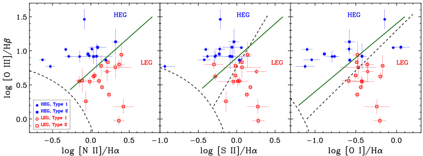
Figure 6.— Emission-line flux ratios. Seyfert, LINER, and star-forming galaxies classifications are indicated by dashed lines following Kewley et al. (2006). YRGs are classified into two groups: HEGs (filled blue symbols) and LEGs (open red symbols), while Type 1 (Type 2) objects are denoted by circle (rectangle) symbols. The dividing lines between HEGs and LEGs are indicated by green solid lines. (A color version of this figure is available in the online journal.)

4.1. Black Hole Mass

We determine BH masses ($M_{\mathrm{BH}}$) using two different methods for Type 1 and Type 2 AGNs, respectively. For 10 Type 1 AGNs with detected broad emission lines, we estimate $M_{\mathrm{BH}}$ based on the virial assumption of the broad-line region (e.g., Woo & Urry 2002; McGill et al. 2008; Shen et al. 2008). In practice, we used the single-epoch mass estimator from McGill et al. (2008):

$$M_{\mathrm{BH}}/{\rm M}_{\odot} = 10^{7.21}\left(\frac{\sigma_{\rm H\alpha}}{10^{3}~{}\mathrm{km~{}s^{-1}}}\right)^{2}\left(\frac{L_{\rm H\alpha}}{10^{42}~{}\mathrm{erg~{}s^{-1}}}\right)^{0.55},$$ (1)

where $\sigma_{\rm H\alpha}$ is the line dispersion of broad H$\alpha$, and L_Hα is the broad H$\alpha$ luminosity. Table 4 lists the determined $M_{\mathrm{BH}}$ along with the luminosity and line dispersion of broad H$\alpha$ for 10 Type 1 AGNs.

Since there are several recipes of $M_{\mathrm{BH}}$ estimation based on different calibrations, we also estimated $M_{\mathrm{BH}}$for comparison using the single-epoch mass estimator from Park et al. (2012) with the virial coefficient determined from the $M_{\mathrm{BH}}-\sigma_{*}$ relation of the reverberation sample (Woo et al. 2010):

$$M_{\mathrm{BH}}/{\rm M}_{\odot} = 10^{7.60}\left(\frac{\sigma_{\mathrm{H}\beta}}{10^{3}~{}\mathrm{km~{}s^{-1}}}\right)^{2}\left(\frac{\lambda L_{5100}}{10^{44}~{}\mathrm{erg~{}s^{-1}}}\right)^{0.52},$$ (2)

where $\sigma_{\mathrm{H}\beta}$ is the line dispersion of broad H$\beta$, and L₅₁₀₀ is AGN continuum luminosity at 5100 Å. Since broad H$\beta$ is relatively weak and detected only for 7 objects, we inferred $\sigma_{H\beta}$ from $\sigma_{H\alpha}$, using the correlation between H$\alpha$ and H$\beta$ line widths (Equation (3) in Greene & Ho 2005). In the case of L₅₁₀₀, we used the correlation between L_Hα and L₅₁₀₀ given by Greene & Ho (2005). $M_{\mathrm{BH}}$ estimated in this method is systematically larger than that determined with Equation (1) by $\sim 26\%$ due to the different calibrations between luminosities and/or line widths adopted in the mass estimators. However, the systematic difference is relatively small compared to the large range of mass and luminosity of the sample, and does not significantly affect the main results.

For objects with measured $\sigma_{*}$, we derive $M_{\mathrm{BH}}$ from $\sigma_{\ast}$ using the $M_{\mathrm{BH}}-\sigma_{\ast}$ relation of early-type galaxies (Gültekin et al. 2009):

$$\log M_{\mathrm{BH}}/{\rm M}_{\odot}=8.22+3.86\log(\sigma_{\ast}/{200~{}\mathrm{km~{}s^{-1}}}).$$ (3)

For two Type 1 AGN 0942+355 and 1601+528, $M_{\mathrm{BH}}$ was determined with both methods, however, we adopted $M_{\mathrm{BH}}$ estimates from the $M_{\mathrm{BH}}-\sigma_{*}$ relation since the systematic uncertainties in Equation (1) and (2) due to dust extinction and indirect estimates of the broad-line size from H$\alpha$ luminosity are probably large for these Type 1 AGNs with relatively redder spectral energy distributions (SEDs). In summary, $M_{\mathrm{BH}}$ was determined from measured $\sigma_{\ast}$ for 24 Type 2 objects and 2 Type 1 objects as listed in Table 5. The $M_{\mathrm{BH}}$ of the YRGs in our sample ranges over two orders of magnitude, $7.0<{\rm log(M_{\mathrm{BH}}/{\rm M}_{\odot})}<9.2$, indicating that YRGs host relatively massive BHs, similar to the large-scale radio galaxies.

Table 4$M_{\mathrm{BH}}$ and gas properties of Type 1 AGNs

Name	log $L_{H\alpha}$	$\sigma_{H\alpha}$	log $M_{\mathrm{BH}}$	log $T_{e}$	log $n_{e}$
	(erg s-1)	(km s-1)	(${\rm M}_{\odot}$)	(K)	(cm-3)
(1)	(2)	(3)	(4)	(5)	(6)
0134+329	43.8	1549	8.6	$\cdots$	$\cdots$
0221+276	42.7	3531	8.7	4.4	3.4
0316+413	41.6	1032	7.0	$\cdots$	2.9
0942+355	42.2	1323	7.5	$\cdots$	2.5
1154+435	42.8	1268	7.9	4.3	2.5
1203+645	42.8	2567	8.4	4.1	$\cdots$
1250+568	43.2	1705	8.3	4.6	$\cdots$
1345+125	41.8	1307	7.3	$\cdots$	$\cdots$
1404+286	42.6	3990	8.7	$\cdots$	$\cdots$
1601+528	41.5	1139	7.1	$\cdots$	$\cdots$

Note. — Columns: (1) Target name; (2) Luminosity of the broad H$\alpha$; (3) Line dispersion of the broad H$\alpha$; (4) $M_{\mathrm{BH}}$ estimated with single epoch method; (5) Electron temperature estimated from [O iii] ratio (I(4959+5007)/I(4363)), assuming electron density of $n_{e}\sim 10^{3}$ cm^-3; (6) Electron density estimated from the [S ii] ratio of I(6716)/I(6731), assuming an electron temperature of $10^{4}$ K.

Table 5$M_{\mathrm{BH}}$ and gas properties of Type 2 AGNs

Name	$\sigma_{\ast}$	log $M_{\mathrm{BH}}$	log $T_{e}$	log $n_{e}$
	(km s-1)	(${\rm M}_{\odot}$)	(K)	(cm-3)
(1)	(2)	(3)	(4)	(5)
0019$-$000	329 $\pm$ 114	9.1	$\cdots$	$\cdots$
0025+006	108 $\pm$ 10	7.2	$\cdots$	2.3
0035+227	222 $\pm$ 7	8.4	$\cdots$	$\cdots$
0345+337	258 $\pm$ 26	8.6	$\cdots$	$\cdots$
0428+205	263 $\pm$ 26	8.7	$\cdots$	2.9
0605+480	360 $\pm$ 42	9.2	$\cdots$	2.2
0754+401	122 $\pm$ 7	7.4	4.1	2.5
0810+077	233 $\pm$ 14	8.5	$\cdots$	2.6
0921+143	248 $\pm$ 19	8.6	$\cdots$	3.1
0931+033	341 $\pm$ 24	9.1	$\cdots$	2.8
0941$-$080	148 $\pm$ 17‡	7.7	$\cdots$	3.2
0942+355†	120 $\pm$ 17	7.4	$\cdots$	$\cdots$
1007+142	344 $\pm$ 43	9.1	$\cdots$	2.8
1037+302	199 $\pm$ 14	8.2	$\cdots$	1.6
1225+442	184 $\pm$ 59	8.1	$\cdots$	2.8
1233+418	166 $\pm$ 22	7.9	$\cdots$	$\cdots$
1245+676	233 $\pm$ 2	8.5	$\cdots$	2.7
1323+321	353 $\pm$ 79	9.2	4.1	$\cdots$
1407+363	154 $\pm$ 19	7.8	$\cdots$	2.9
1521+324	118 $\pm$ 11	7.3	$\cdots$	3.1
1558+536	229 $\pm$ 30	8.4	$\cdots$	3.2
1601+528†	240 $\pm$ 15	8.5	$\cdots$	$\cdots$
1610+407	201 $\pm$ 24	8.2	$\cdots$	$\cdots$
1807+698	258 $\pm$ 21	8.6	$\cdots$	$\cdots$
1943+546	234 $\pm$ 28	8.5	$\cdots$	$\cdots$
2352+495	246 $\pm$ 14	8.6	$\cdots$	$\cdots$

Note. — Columns: (1) Target name. ^†Type 1 AGN; (2) Stellar velocity dispersion. ^‡We adopted the measurement from Snellen et al. (2003).; (3) $M_{\mathrm{BH}}$ estimated from the $M_{\mathrm{BH}}-\sigma_{\ast}$ relation: (4) Electron temperature estimated from [O iii] ratio (I(4959+5007)/I(4363)), assuming electron density of $n_{e}\sim 10^{3}$ cm^-3; (5) Electron density estimated from the [S ii] ratio of I(6716)/I(6731), assuming an electron temperature of $10^{4}$ K.

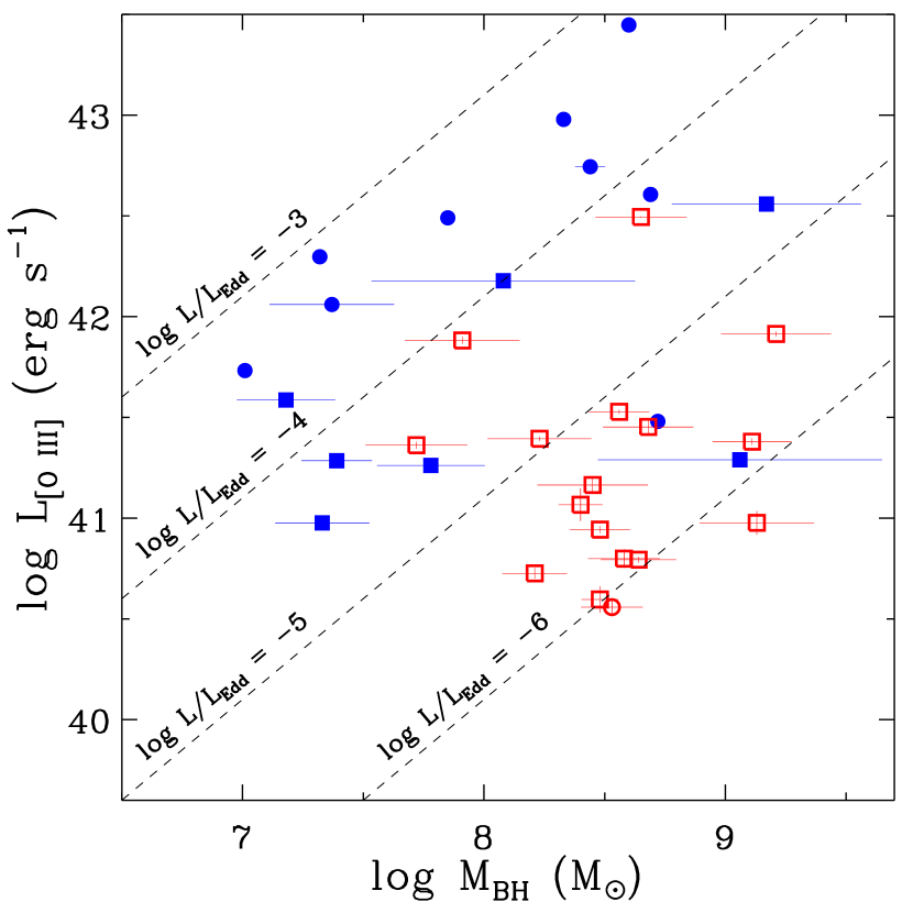
Figure 7.— Comparison of the [O iii] line luminosity with $M_{\mathrm{BH}}$. Symbols are the same as in Figure 6. Dashed lines indicate the ratio of line luminosity to the Eddington limit. (A color version of this figure is available in the online journal.)

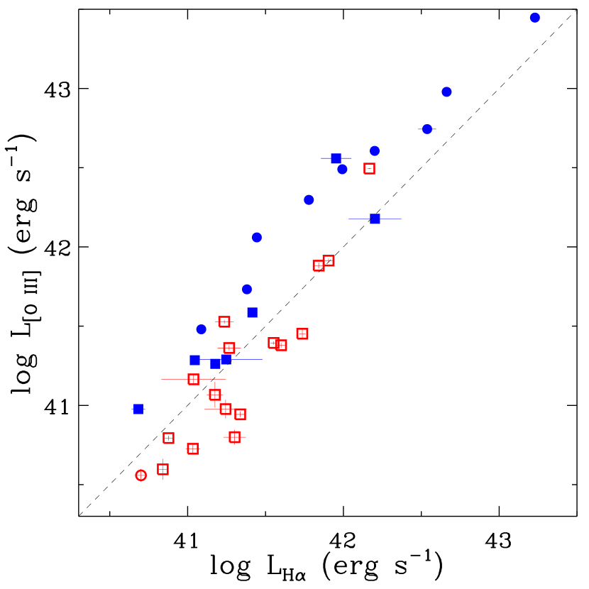
Figure 8.— H$\alpha$ vs. [O iii] line luminosities. Note that HEGs (filled symbols) have higher [O iii] luminosity than LEGs (open symbols) at fixed H$\alpha$ luminosity as expected from higher [O iii]/H$\beta$ ratio. (A color version of this figure is available in the online journal.)

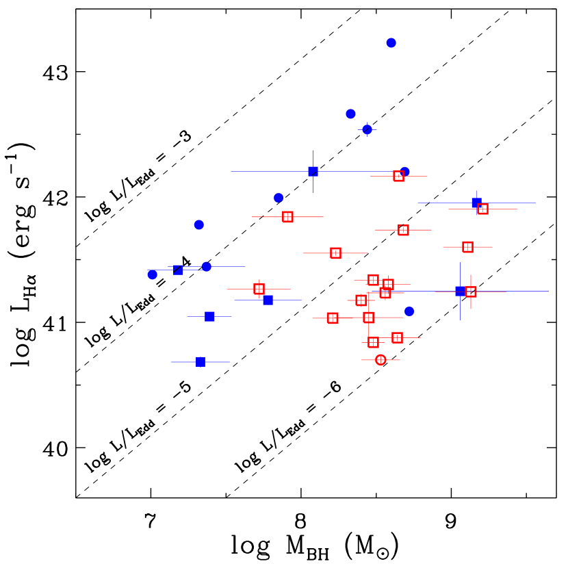
Figure 9.— Comparison of the H$\alpha$ line luminosity with $M_{\mathrm{BH}}$. Symbols are the same as in Figure 6. Dashed lines indicate the ratio of line luminosity to the Eddington limit. (A color version of this figure is available in the online journal.)

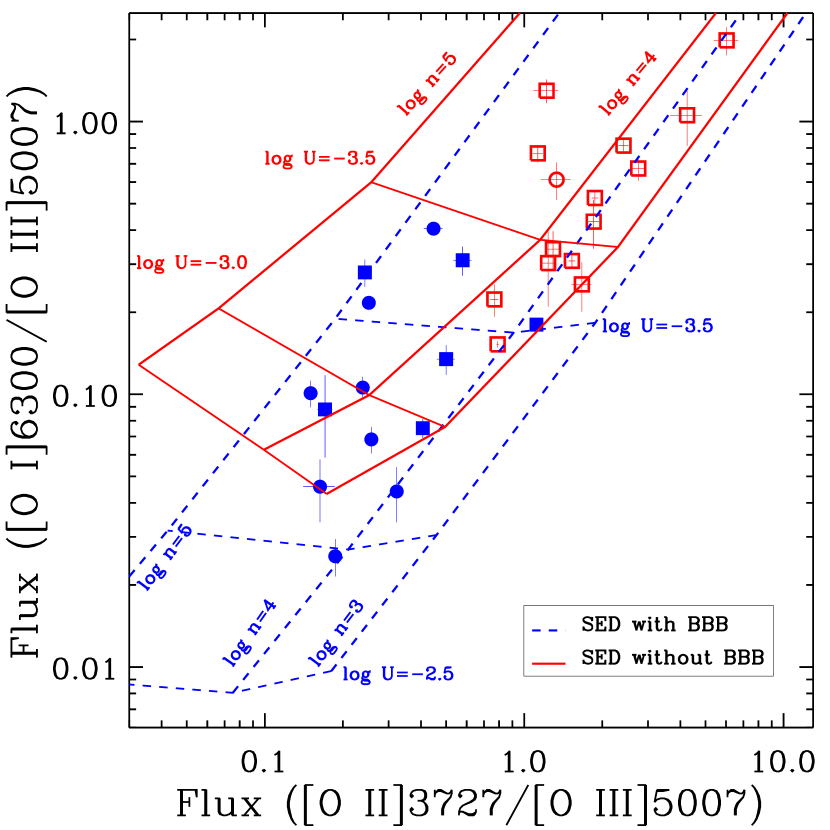
Figure 10.— [O i]$\lambda$6300/[O iii]$\lambda$5007 vs. [O ii]$\lambda$3727/[O iii]$\lambda$5007 ratios. The measured line ratios of HEGs (filled symbols) and LEGs (open symbols) are compared with photoionization model predictions with a SED with BBB (blue lines) and a SED without BBB (red lines), respectively. The assumed ionization parameters (log U) and hydrogen densities (log n) are denoted by different lines. (A color version of this figure is available in the online journal.)

4.2. Narrow-line Region

4.2.1 Excitation and Accretion

To investigate the properties of accretion activities in YRGs, we compare the flux ratios of high and low excitation lines in Figure 6. All YRGs in our sample are classified as AGNs based on the criteria of Kewley et al. (2006), suggesting that photoionization by a nuclear source is a main mechanism of narrow line emission in YRGs. There is a wide range of line flux ratios, which are generally divided into Seyfert and LINER (Low-Ionization Nuclear Emission-line Region) classes in radio-quiet (RQ) Type 2 AGNs as indicated by diagonal dashed lines.

We classify YRGs into two groups: HEGs and LEGs based on the flux ratios between high- and low-excitation lines using the excitation index (EI) suggested by Buttiglione et al. (2010),

$$\scriptsize{\rm EI}=\log{\rm[O~{}III]\over H\beta}-{1\over 3}\left(\log{\rm[N~{}II]\over H\alpha}+\log{\rm[S~{}II]\over H\alpha}+\log{\rm[O~{}I]\over H\alpha}\right),$$

which represents the average ratio of high to low excitation line fluxes. If EI is larger (smaller) than 0.95, YRGs are classified as HEG (LEG). For five objects (0019-000, 0035+227, 0942+355, 1225+442, and 1245+676), not all three high-excitation lines (i.e., [N II], [S II] and [O I]) were measured, thus, we used only one or two available lines for classification as suggested by Buttiglione et al. (2010).

1943+546 is excluded since none of the three low-ionization lines were detected. We note that 0345+337 is classified as LEG, while it was previously classified as HEG by Buttiglione et al. (2010), presumably owing to the lower quality of their spectra.

In summary, the YRG sample consists of 16 HEGs, 17 LEGs, and 1 unclassified object. All Type 1 AGNs with broad H$\alpha$ belong to the HEG class except for 1601+528, while Type 2 AGNs belong to both HEG and LEG classes. These trends are similar to those found in FR I and FR II galaxies. For example, Buttiglione et al. (2010) showed that all Type 1 objects in their 3CR sample were HEGs, while Type 2 objects were composed of both HEGs and LEGs.

4.2.2 Accretion Rate vs. High-to-low Excitation Line Ratio

We investigate whether HEGs and LEGs have systematically different accretion activity by comparing their Eddington ratios. Since bolometric luminosity cannot be directly measured for Type 2 AGNs, first, we use the [O iii] line luminosity as a proxy for bolometric luminosity. In Figure 7 we compare the [O iii] luminosity with $M_{\mathrm{BH}}$. At fixed $M_{\mathrm{BH}}$, HEGs have higher line luminosities than LEGs, suggesting that HEGs have higher Eddington ratios. Although, the separation between HEGs and LEGs is not a clear cut, the average Eddington ratio of HEGs is $\sim$1.2 dex larger than that of LEGs.

However, [O iii] may not be a good indicator of bolometric luminosity, particularly when HEGs and LEGs are compared since HEGs have relatively higher [O iii]/H$\beta$ ratio than LEGs. Thus, bolometric luminosity based on [O iii] can be systematically overestimated for HEGs. Also, an orientation dependency of [O iii] has been reported as that for given isotropic flux (e.g., far-infrared or [OIV] 25.9µm) the [O iii] line flux of Type 2 AGNs is systematically lower than that of Type 1 AGNs (Jackson & Browne 1990; Nagao et al. 2001; Haas et al. 2005; Baum et al. 2010), suggesting a bias of [O iii] as a bolometric luminosity indicator. A recent study by Netzer (2009) reported that bolometric correction of [O iii] systematically changes as a function of [O iii]/H$\beta$ ratio, while H$\alpha$ does not show such a trend, indicating that H$\alpha$ is a better tracer of bolometric luminosity.

To test the systematic difference between [O iii] and H$\alpha$, we compare them in Figure 8. As expected, HEGs have higher [O iii] luminosity for given H$\alpha$ luminosity, while LEGs have lower [O iii] luminosity for given H$\alpha$ luminosity. This result indicates that if the luminosity of [O iii] is used as a proxy for AGN bolometric luminosity, the difference of bolometric luminosity between HEGs and LEGs would be overestimated.

In Figure 9 we compare $M_{\mathrm{BH}}$ with the H$\alpha$ luminosity. The average difference between HEGs and LEGs decreases compared to Figure 7. However, we find that the average Eddington ratio of HEGs is still larger than that of LEGs by $\sim$1.0 dex (a factor of 9.0). The difference of the Eddington ratio suggests that HEGs may have higher mass accretion rate at fixed $M_{\mathrm{BH}}$ than LEGs or that radiative efficiency is systematically different if the mass accretion rate normalized by $M_{\mathrm{BH}}$ is similar.

4.2.3 Comparison with Photoionization Models

We investigate whether HEGs and LEGs have different types of photoionizing continua by comparing observed emission-line flux ratios with photoionization models. Using Cloudy version 08.00 (Ferland et al. 1998), we calculate the ratios of various emission lines arising in the NLR gas clouds. We assume the NLR metallicity $Z_{\rm NLR}=2Z_{\sun}$ since such a super-solar metallicity has been generally reported for the NLRs (e.g., Nagao et al. 2006), and investigate line flux ratios with a density range of $n_{\rm H}=10^{2.0}-10^{5.0}$ and an ionization parameter range of $\log U=10^{-4.0}-10^{-2.5}$ that are typical for NLRs (e.g., Nagao et al. 2001). In the case of photoionizing sources, we used two types of SEDs: SED with big blue bump (BBB) and SED without BBB (see Nagao et al. 2002; Kawakatu et al. 2009). Note that the SED without BBB can be expressed with a single power-law continuum (harder spectrum) in the range of $\sim$10¹² to $\sim$10²⁰ Hz. Such a harder spectrum of the optically thin disk (radiatively inefficient accretion flow) generates different line ratio compared to the SED with BBB, as presented in Figure 10. At fixed $U$ and $n_{\rm H}$, the photoionization models using SED with BBB (blue lines) predict lower [O i]$\lambda$6300/[O iii]$\lambda$5007 than the models using SED without BBB (red lines), as also summarized by Kawakatu et al. (2009; see Section 4.1).

We compare the measured line flux ratios of [O i]$\lambda$6300/[O iii]$\lambda$5007 and [O ii]$\lambda$3727/[O iii]$\lambda$5007 with model predictions in Figure 10, where HEGs and LEGs are located in different regions. For HEGs, [O iii]$\lambda$5007 is stronger than [O i]$\lambda$6300 or [O ii]$\lambda$3727 lines, consistent with the photoionization model calculations using SEDs with BBB. In contrast, for LEGs [O iii]$\lambda$5007 is relatively weak compared to [O i]$\lambda$6300 or [O ii]$\lambda$3727 lines, suggesting that the measured line flux ratios of LEGs are consistent with models predictions using SEDs without BBB. We may interpret these findings as that HEGs generally have radiatively efficient accretion disk with BBB, while LEGs have radiatively inefficient disk without BBB. In other words, high and low excitation can be related with the properties of accretion disk.

In the case of SDSS Seyfert 2 galaxies, [O iii]$\lambda$5007 is relatively stronger than [O i]$\lambda$6300 or [O ii]$\lambda$3727, which is consistent with SED with BBB (see Kawakatu et al. 2009). Thus, high-excitation YRGs and Seyfert 2 galaxies may have similar accretion properties. Kawakatu et al. (2009) suggested that YRGs have radiatively inefficient accretion disk based on the small sample of YRGs, of which the oxygen line flux ratios were consistent with photoionization model without BBB. However, note that their sample was mostly composed of LEGs. In contrast, in this work, we include many Type 1 AGNs with relatively higher Eddington ratios, which are mostly HEGs, leading to a more general view on the accretion properties of YRGs.

The different location on the oxygen line ratio diagram can also be interpreted as that LEGs have relatively lower ionization parameter than HEGs, while both classes have similar ionizing SEDs. We cannot rule out this possibility with the current data. To break the degeneracy between the SED shape and the ionization parameter, we attempted to measure [Ar iii]/[O iii] ratio, which is a robust indicator of the ionization parameter, independent of SED shapes (Nagao et al. 2002). Unfortunately, [Ar iii] is generally very weak and we are not able to detect [Ar iii] in most of LEGs, leading to inconclusive results (see Table 3).

4.2.4 Gas Properties

We estimated the electron temperature ($T_{e}$) and density ($n_{e}$) of the NLR using emission-line ratios. The [O iii] flux ratio, I(4363)/I(4959+5007) is generally used as an indicator of $T_{e}$, while the flux ratio of [S ii], I(6716)/I(6731) is used for estimating $n_{e}$ (Osterbrock & Ferland 2006). We used the temden task in the IRAF nebular package to calculate $T_{e}$ and $n_{e}$. For six objects we were able to estimate $T_{e}$ in the ranges of $4.0\leq\log T_{e}\leq 4.6$, assuming $n_{e}=10^{3}$ cm^-3.

For measuring electron density, [S ii] ratios were determined for 20 objects, ranging from $0.7$ to $1.4$, which corresponded to $\log n_{e}\approx 1.6-3.4$ cm^-3, assuming $n_{e}=10^{4}$ K. For the remaining galaxies, the electron density could not be calculated due to the failure of deblending of [S ii]$\lambda$6717 & [S ii]$\lambda$6731 lines, We find that electron temperature and density of the NLRs in YRGs are similar to typical RQ AGNs. The estimated electron temperature and density of NLR are listed in Table 4 and 5.

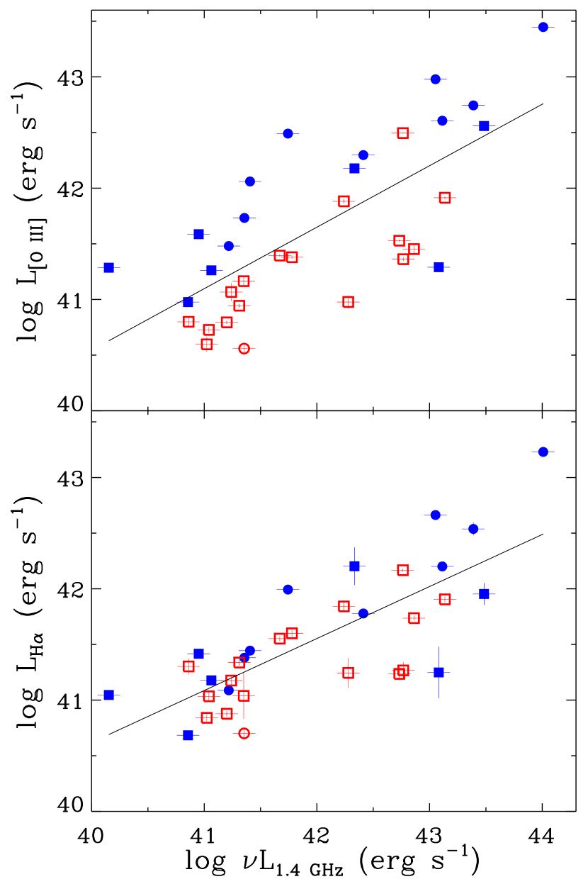
Figure 11.— Comparison of radio core luminosity with the [O iii] (top) and H$\alpha$ line luminosities (bottom). Symbols are the same as in Figure 6. The measurements errors of radio luminosities are assumed to 0.1 dex. (A color version of this figure is available in the online journal.)

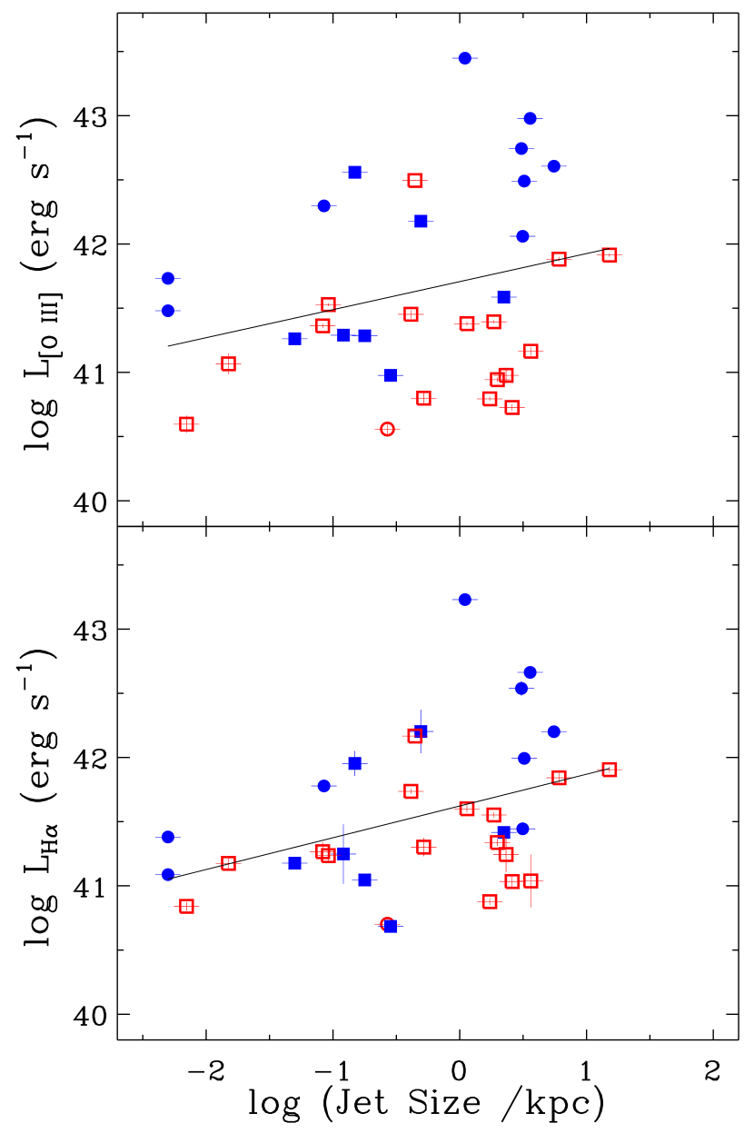
Figure 12.— Comparison of the jet size with the [O iii] (top) and H$\alpha$ line luminosities (bottom). Symbols are the same as in Figure 6. (A color version of this figure is available in the online journal.)

4.3. Radio jet properties

We investigate the connection between radio and accretion activities by comparing radio luminosity and jet size with [O iii] and H$\alpha$ luminosities. Figure 11 compares the radio core luminosity with the line luminosities of [O iii] and H$\alpha$. In general there is a broad correlation between radio and narrow emission-line luminosities. If we consider narrow-line luminosity as a proxy for AGN bolometric luminosity as discussed in Section 4.2, the broad correlation indicates that radio and accretion activities are fundamentally connected in YRGs. A similar trend has been reported in large-scale radio galaxies (i.e., FR Is and FR IIs) by a number of previous studies (e.g. Baum & Heckman 1989; Rawlings & Saunders 1991; Buttiglione et al. 2010).

Comparing HEGs and LEGs at fixed radio luminosity, we find HEGs have higher [O iii] luminosity than LEGs, suggesting that accretion properties are different between HEGs and LEGs although radio activities are similar. It is possible that there is a second parameter to change the accretion power at given radio power. These trends were also reported for large-scale radio galaxies by Buttiglione et al. (2010), who investigated the radio and emission-line luminosities of a sample of low-z 3C radio galaxies (see also Kunert-Bajaraszewska & Labiano 2010). They argued that the separation between HEGs and LEGs is due to the different temperature of the accreting gas. While HEGs have inflow of cold gas, LEGs accrete hot gas, resulting in a harder photoionizing spectrum and stronger low-excitation lines than those of HEGs.

If the [O iii] line flux is systematically higher than the H$\alpha$ line flux in HEGs as discussed in Section 4.2 (see Figure 8), then the difference between HEGs and LEGs may be overestimated. To overcome this systematic uncertainty, we also use the H$\alpha$ luminosity as a proxy for bolometric luminosity for investigating whether HEGs and LEGs have different accretion properties at fixed radio luminosity. When [O iii] is replaced by H$\alpha$ (bottom panel of Figure 11), the separation between HEGs and LEGs is less clear although on average HEGs have higher H$\alpha$ luminosity than LEGs. Since the division between HEGs and LEGs is not distinct, we derive the correlation for the combined sample of HEGs and LEGs using a least square fitting method:

$$\log\rm L_{H\alpha}=(21.9\pm 3.0)+(0.5\pm 0.1)\log\nu\rm L_{1.4}.$$ (5)

The correlation has 0.4 dex scatter, indicating that accretion luminosity can vary by more than a factor of two at given radio luminosity. The correlation between narrow-line and radio luminosities found in YRGs seems similar to that of large-scale radio galaxies. However, the slope of the correlation in large-scale radio galaxies is close to 1, which somewhat steeper than that of YRGs (Buttiglione et al. 2010).

By comparing the linear jet size with the [O iii] and H$\alpha$ luminosities in Figure 12, we find a weak correlation between emission-line luminosity and the projected jet size, as similarly reported by Labiano (2008) for GPS and CSS sources. However, the correlation is not very tight with considerably large scatter in the case of [O iii]. When the H$\alpha$ luminosity is compared with the jet size, the relation becomes slightly tighter with 0.5 dex scatter, probably due to the systematic difference of [O iii]/H$\alpha$ ratios between HEGs and LEGs. We derive the correlation between H$\alpha$ luminosity and jet size as:

$$\log\rm L_{H\alpha}=(41.6\pm 0.1)+(0.2\pm 0.1)\log(R_{jet}/kpc),$$ (6)

where R_jet is the size of jet in kpc. Note that since the jet size is measured as a projected size, the true jet size may be larger, implying that the correlation is even weaker. The shallow slope of the relation indicates that YRGs with similar emission line luminosities and accretion rates can have dramatically different jet sizes, implying that the jet size may be determined by other mechanisms, e.g., the properties of interstellar medium in the host galaxies than accretion properties. We further investigate whether the HEG/LEG ratio changes as a function of the jet size using our YRG sample and 3CR radio galaxies from Buttiglione et al. (2010). No significant change of the ratio has been detected over the large range of the jet size ($\sim$10 pc to $\sim$1 Mpc), suggesting that the jet size is not directly connected to the properties of the accretion flows. These findings are consistent with a scenario that accretion properties can change over the lifetime of radio jets.

5. DISCUSSIONS AND SUMMARY

To investigate spectral properties of YRGs and compare them with radio properties, we construct a sample of 34 YRGs at relatively low redshift ($z<0.4$) for measuring narrow emission-line properties, $M_{\mathrm{BH}}$, and Eddington ratio. We determined $M_{\mathrm{BH}}$ from the width and luminosity of the broad H$\alpha$ line using single-epoch mass estimators for Type 1 (broad-line) AGNs, or from the measured stellar velocity dispersion using the $M_{\mathrm{BH}}-\sigma_{*}$ relation for Type 2 (narrow-line) AGNs. The estimated $M_{\mathrm{BH}}$ ranges from 10^7.0 to 10^9.2 ${\rm M}_{\odot}$, indicating YRGs have relatively massive BHs, similar to the large-scale radio galaxies.

Based on the narrow emission-line flux ratios (e.g. [O iii]/H$\beta$, [N ii]/H$\alpha$, [S ii]/H$\alpha$, and [O i]/H$\alpha$), we classified YRGs as HEG and LEG. Most of Type 1 AGNs belong to HEGs, while Type 2 AGNs are composed of HEGs and LEGs. We find that the Eddington ratio of HEGs is higher by $\sim$1.0 dex than that of LEGs, using the H$\alpha$ line luminosity as a proxy for AGN bolometric luminosity. The difference in Eddington ratios and comparison with photoionization models suggest that HEGs are high Eddington ratio AGNs with an optically thick accretion disk, which are similar to QSOs or Seyfert 1 galaxies, while LEGs have lower Eddington ratios with radiatively inefficient accretion flow. This interpretation is similar to the division between Seyfert galaxies and LINERs in RQ AGNs (Kewley et al. 2006; Ho 2008), suggesting that YRGs have a various range of accretion activities over 2-3 orders of magnitude in the Eddington ratio.

Kawakatu et al. (2009) investigated whether the optical narrow emission-line ratios of YRGs are systematically different from those of RQ Seyfert 2 galaxies by comparing the observed line ratios (e.g., [O i]/[O iii] and [O ii]/[O iii]) with photoionization models. Using a limited sample of YRGs, they concluded that YRGs favor SED without a strong BBB, i.e., optically thin advection-dominated accretion flow, while RQ AGNs are consistent with the models adopting SED with a strong BBB, i.e., a geometrically thin, optically thick disk. In this study with an enlarged sample including Type 1 AGNs with higher Eddington ratios, we find that there are various levels of accretion activity in YRGs and that both SEDs with/without BBB are required to reproduce the observed line flux ratios of YRGs.

Low luminosity AGNs, i.e., LINERs, generally tend to be radio-loud (Ho 1999, Terashima & Wilson 2003), implying that radio activity may be related with radiatively inefficient accretion flow, similar to the low-state in X-ray binaries (McClintock & Remillard 2006). In the case of YRGs, we find a large range of Eddington ratios, including HEGs with high accretion power and Seyfert-like emission-line flux ratios. Thus, the connection between radio jet and radiatively inefficient accretion flow is not strong in YRGs. Instead, YRGs are probably composed of heterogeneous objects representing various accretion states.

By comparing narrow emission-line properties with radio luminosity and jet size, we investigated the disk-jet connection in YRGs. The [O iii] and H$\alpha$ line luminosities show broad correlations with the radio core luminosity, indicating that accretion and radio activities in YRGs are fundamentally linked. However, at fixed radio luminosity, HEGs have higher line luminosities (particularly for [O iii]) than LEGs, indicating that HEGs have higher accretion activity than LEGs for a given radio activity. These results may suggest that at a given radio activity there is a continuous distribution of accretion powers due to various mass accretion rate.

References

- (1) Abazajian, K. N., Adelman-McCarthy, J. K., Agüeros, M. A., et al. 2009, ApJS, 182, 543
- (2) Alexander, P., & Leahy, J. P. 1987, MNRAS, 225, 1
- (3) Axon, D. J., Capetti, A., Fanti, R., et al. 2000, AJ, 120, 2284
- (4) Barth, A. J., Ho, L. C., Sargent, W. L. W. 2002, AJ, 124, 2607
- (5) Baum, S. A., & Heckman, T. 1989, ApJ, 336, 681
- (6) Baum, S. A., Gallimore, J. F., O’Dea, C. P., et al. 2010, ApJ, 710, 289
- (7) Bennert, V. N., Auger, M. W., Treu, T., et al. 2011, ApJ, 726, 59
- (8) Boroson, T. A., & Green, R. F. 1992, ApJS, 80, 109
- (9) Buttiglione, S., Capetti, A., Celotti, A., et al. 2009, A&A, 495, 1033
- (10) Buttiglione, S., Capetti, A., Celotti, A., et al. 2010, A&A, 509, 6
- (11) Cardelli, J. A., Clayton, G. C., & Mathis, J. S. 1989, ApJ, 345, 245
- (12) Carilli, C. L., Perley, R. A., Dreher, J. W., & Leahy, J. P. 1991, ApJ, 383, 554
- (13) de Vries, W. H., O’Dea, C. P., Baum, S. A., & Barthel, P. D. 1999, ApJ, 526, 27
- (14) Fanti, C. 2009, Astron. Nachr., 330, 120
- (15) Fanti, C., Fanti, R., Dallacasa, D., et al. 1995, A&A, 302, 317
- (16) Fender, R. P., Belloni, T. M. & Gallo, E. 2004, MNRAS, 335, 1105
- (17) Ferland, G. J., Korista, K. T., Verner, D. A., et al. 1998, PASP, 110, 761
- (18) Ferrarese, L., & Merritt, D. 2000, ApJ, 539, L9
- (19) Gelderman, R., & Whittle, M. 1994, ApJS, 91, 491
- (20) Giroletti M., & Polatidis, A. 2009, Astron. Nachr., 330, 193
- (21) Greene, J. E., & Ho, L. C. 2005, ApJ, 630, 122
- (22) Gültekin, K., Richstone, D. O., Gebhardt, K., et al. 2009, ApJ, 698, 198
- (23) Ho, L. C. 1999, ApJ, 516, 672
- (24) Ho, L. C. 2008, ARA&A, 46, 475
- (25) Jackson, N., & Browne, I. W. A. 1990, Nature, 343, 43
- (26) Kawakatu, N., Nagai, H., & Kino, M. 2008, ApJ, 687, 141
- (27) Kawakatu, N., Nagao, T., & Woo, J.-H. 2009, ApJ, 693, 1686
- (28) Kewley, L. J., Groves, B., Kauffmann, G., & Heckman, T. 2006, MNRAS, 372, 961
- (29) Komissarov, S. S., Barkov, M. V., Vlahakis, N., & Königl, A. 2007, MNRAS, 380, 51
- (30) Kunert-Bajaraszewska, M., Gawronski, M. P., Labiano, A., & Siemiginowska, A. 2010, MNRAS, 408, 2261
- (31) Kunert-Bajaraszewska, M., & Labiano, A. 2010, MNRAS, 408, 2279
- (32) Labiano, A. 2008, A&A, 488, L59
- (33) Labiano, A., O’Dea, C. P., Gelderman, R., et al. 2005, A&A, 436, 493
- (34) Laing, R. A., Jenkins, C. R., Wall, J. V., & Unger, S. W. 1994, in ASP Conf. Ser. 54, The First Stromlo Symposium: The Physics of Active Galaxies, ed. G. V. Bicknell, M. A. Dopita, & P. J. Quinn (San Francisco, CA: ASP), 201
- (35) Markwardt, C. B. 2008, in ASP Conf. Ser. 411, Astronomical Data Analysis Software and Systems XVIII, ed. D. Bohlender, P. Dowler & D. Durand (San Francisco, CA:ASP), 251
- (36) McClintock, J. E., & Remillard, R. A. 2006, Compact Stellar X-ray Sources (Cambridge: Cambridge Univ. Press), 157
- (37) McGill, K. L., Woo, J.-H., Treu, T., & Malkan, M. A. 2008, ApJ, 673, 703
- (38) McKinney, J. C. 2006, MNRAS, 368, 1561
- (39) McKinney, J. C., Tchekhovskoy, A., & Blandford, R. D. 2012, MNRAS, 423, 3083
- (40) Meier, D. L. 2003, New Astron. Rev., 47, 667
- (41) Miller, J. S., & Stone, R. P. S. 1993, Lick Obs. Tech. Rep. No. 66
- (42) Morganti, R., Ulrich, M.-H., & Tadhunter, C. N. 1992, MNRAS, 254, 546
- (43) Nagao, T., Maiolino, R., & Marconi, A. 2006, A&A, 447, 863
- (44) Nagao, T., Murayama, T., Shioya, Y., & Taniguchi, Y. 2002, ApJ, 567, 73
- (45) Nagao, T., Murayama, T., & Taniguchi, Y. 2001, ApJ, 546, 744
- (46) Netzer, H. 2009, MNRAS, 399, 1907
- (47) O’Dea, C. P. 1998, PASP, 110, 493
- (48) O’Dea, C. P., Daly, R. A., Kharb, P., Freeman, K. A., & Baum, S. A. 2009, A&A, 494, 471
- (49) O’Dea, C. P., de Vries, W. H., Koekemoer, A. M., et al. 2002, ApJ, 123, 2333
- (50) Oke, J. B., & Gunn, J. E. 1982, PASP, 94, 586
- (51) Orienti, M., Dallacasa, D., & Stanghellini, C. 2007, A&A, 475, 813
- (52) Osterbrock, D. E., & Ferland, G. J. 2006, Astrophysics of Gaseous Nebulae and Active Galactic Nuclei (2nd ed.; Sausalito, CA: Univ. Science Books)
- (53) Park, D., Woo, J.-H., Treu, T., et al. 2012, ApJ, 747, 30
- (54) Punsly, B., & Zhang, S. 2011, ApJL, 735, L3
- (55) Rawlings, S., & Saunders, R. 1991, Nature, 349, 138
- (56) Rees, M. J. 1984 ARA&A, 22, 471
- (57) Remillard, R. A., & McClintock, J. E. 2006, ARA&A, 44 , 49
- (58) Shen, Y., Greene, J. E., Strauss, M. A., Richards, G. T., & Schneider, D. P. 2008, ApJ, 680, 169
- (59) Snellen, I. A. G., Lehnert, M. D., Bremer, M. N., & Schilizzi, R. T. 2003, MNRAS, 342, 889
- (60) Suyu, S. H., Marshall, P. J., Auger, M. W., et al. 2010, ApJ, 711, 201
- (61) Terashima, Y., & Wilson, A. S. 2003, ApJ, 583, 145
- (62) Woo, J.-H., Treu, T., Barth, A.J., et al. 2010, ApJ, 716, 269
- (63) Woo, J.-H., Treu, T., Malkan, M. A., & Blandford, R. D. 2006, ApJ, 645, 900
- (64) Woo, J.-H., & Urry, C. M. 2002, ApJ, 579, 530
- (65) Woo, J.-H., Urry, C. M., Lira, P., van der Marel, R. P., & Maza, J. 2004, ApJ, 617, 903
- (66) Woo, J.-H., Urry, C. M., van der Marel, R. P., Lira, P., & Maza, J. 2005, ApJ, 631, 762