Quantum gas mixtures in different correlation regimes

Abstract

We present a many-body description for two-component ultracold bosonic gases when one of the species is in the weakly interacting regime and the other is either weakly or strongly interacting. In the one-dimensional limit the latter case system is a hybrid in which a Tonks-Girardeau gas is immersed in a Bose-Einstein condensate, which is an example of a new class of quantum system involving a tunable, superfluid environment. We describe the process of phase separation microscopically and semiclassically in both situations and show that the quantum correlations are maintained in the separated phase.

Introduction – Impurities immersed in ultracold atomic gases have recently emerged as versatile environments for studying quantum correlations in highly controllable systems Cote:02 . Demonstrations of single fermions or single ions embedded in a Bose Einstein condensates (BECs) have shown that such systems are experimentally viable Zipkes:10 , and are paving the way to study a plethora of new quantum phenomena, arising from the interactions between the impurity and the ultracold environment. Better understanding and control of these interactions are already leading to new ideas in quantum information theory Doerk:10 .

Precursors to these highly controllable hybrid systems have been mesoscopic mixtures of ultracold bosonic gases, which consist of either two different atomic species or two different hyperfine states of the same species Myatt:97 . They are commonly available in labs worldwide and have allowed to investigate mesoscopic quantum dynamics in complex systems and to study new exotic states of matter. Such systems have a successful microscopic description based on a two mode model Law:97 and can be approximated semiclassically by using a system of coupled Gross-Pitaevskii equations (GPE) Ho:96 . The latter model allows to describe the stability of the multi-component system Busch:97 and the process of phase separation Ho:96 ; Ao:98 .

In this work we consider a small number of atoms confined in an effectively one-dimensional parabolic trap, which are either in the weakly or in the strongly correlated regime. Because of the reduced dimensionality, the strongly interacting case corresponds to the Tonks-Girardeau (TG) limit Girardeau:60 ; Girardeau:01 , which has recently been demonstrated experimentally Paredes:04 . The same trap contains a second species of atoms, which we consider to be in the weakly correlated regime (the BEC limit), and which acts as a tunable environment for the first component. We show that the quantum correlations can be tuned through the coupling with between the two species, and describe microscopically the phase separation process that drives the immersed species to the edges of the BEC.

A strongly interacting quantum gas in one-dimension can be successfully described in different ways. The first is to use a model of hard sphere bosons and employ a mapping theorem to a non-interacting Fermi gas Girardeau:60 . This permits one to derive an analytical expression for the wave function in position space and only relies on the knowledge of the solutions of the single particle problem Girardeau:60 ; Girardeau:01 ; Goold:10.2 . An equal, but numerically expensive, description is to use a many-body Hamiltonian and expand the field operators into a sufficient number of momenta Deuretzbacher:07 .

Here we choose the second approach and expand the second quantized field operators for both species in a basis of harmonic oscillator functions, including as many momenta as needed. This allows us to microscopically describe the stationary solutions and the phenomenon of phase separation when both species are in the weakly interacting regime (the BEC-BEC limit) and when one is in the strongly interacting regime (the BEC-TG limit). While a larger number of momenta is necessary to describe the TG gas, only a few momenta are necessary for the BEC species, which makes the numerical approach possible. We obtain the many body version of the phase separation criteria and show that this process occurs as a consequence of the excitation of atoms to higher harmonics. The phase separated situation can be treated as a double well potential for the phase separated species and we show that the atoms in the strongly interacting species keep their correlations despite being separated by the BEC component.

Since the above approach is limited to small particle numbers, we generalise the obtained results to the mesoscopic limit by using a semiclassical approach similar to the well known coupled GPE systems Ho:96 . In the BEC-TG limit, however, we show that a GPE coupled to a mean field equation with a quintic Kolomeisky:00 rather than a cubic non-linearity appropriately describes the semiclassical limit, while the non-linearity of the cross term depends on the value of the coupling between the species.

Model – We consider a mixture of two ultracold bosonic species, confined in a quasi-one dimensional (1D) parabolic trap. One component (the ’environment’, $E$) is always in the weakly correlated regime, whereas the other component (the ’system’, $S$) can be either weakly or strongly interacting. The intra-species coupling constants are then given by $g_{E,S}=-2\hbar^{2}/m_{E,S}a_{1D}^{E,S}$, where $m_{E,S}$ are the respective masses of the two components and $a_{1D}^{E,S}=(-(a_{\perp}^{E,S})^{2}/2a_{E,S})[1-C(a_{E,S}/a_{\perp}^{E,S})]$. Here $a_{E,S}$ are the $s$-wave scattering lengths and $a_{\perp}^{E,S}=\sqrt{2\hbar/m_{E,S}\omega_{\perp}}$, where $\omega_{\perp}$ is the trap frequency in the radial direction. The constant $C$ is evaluated in Olshanii:98 . For simplicity we assume that the two components are different hyperfine states of the same atomic species and therefore $m_{E}=m_{S}=M$. The coupling constant between the two components, $g_{ES}$, is given in a similar fashion in terms of the 1D inter-species scattering length, $a_{1D}^{ES}$. We expand the field operators in the second-quantized description of this system Law:97 in terms of the eigenfunctions $\phi_{n}(x)$ of the harmonic potential $V(x)=\frac{1}{2}M\omega^{2}x^{2}$ and use $n_{E,S}$ modes in the expansion for the environment and system component, $\hat{\psi}_{E}(x,t)=\sum_{n=1}^{n_{E}}a_{n}(t)\phi_{n}(x)$ and $\hat{\psi}_{S}(x,t)=\sum_{n=1}^{n_{S}}b_{n}(t)\phi_{n}(x)$. The creation and annihilation operators $a_{k}^{\dagger}$ and $a_{k}$ satisfy the standard (equal time) bosonic commutation relations $[a_{k},a_{l}^{\dagger}]=\delta_{kl},$ $[a_{k},a_{l}]=[a_{k}^{\dagger},a_{l}^{\dagger}]=0$ (and similarly for $b_{k}^{\dagger}$ and $b_{k}$), which yields the Hamiltonian $H=H_{E}+H_{S}+H_{\mathrm{int}}$, where

$$H_{E}= \sum_{k,l}a_{k}^{\dagger}a_{l}H_{kl}+\frac{1}{2}\sum_{klmn}a_{k}^{\dagger}a_{l}^{\dagger}a_{m}a_{n}V_{klmn}^{E}$$ (1)

$$H_{S}= \sum_{k,l}b_{k}^{\dagger}b_{l}H_{kl}+\frac{1}{2}\sum_{klmn}b_{k}^{\dagger}b_{l}^{\dagger}b_{m}b_{n}V_{klmn}^{S},$$ (2)

$$H_{\mathrm{int}}= \frac{1}{2}\sum_{klmn}a_{k}^{\dagger}b_{l}^{\dagger}b_{m}a_{n}V_{klmn}^{ES},$$ (3)

with

$$H_{kl}= \int dx\;\phi_{k}^{*}(x)H_{\mathrm{sp}}\phi_{l}(x),$$ (4)

$$V_{klmn}^{E,S}= \frac{g_{E,S}}{2}\int dx\;\phi_{k}^{*}(x)\phi_{l}^{*}(x)\phi_{m}(x)\phi_{n}(x),$$ (5)

$$V_{klmn}^{ES}= g_{ES}\int dx\;\phi_{k}^{*}(x)\phi_{l}^{*}(x)\phi_{m}(x)\phi_{n}(x).$$ (6)

Here $H_{\mathrm{sp}}$ is the single particle Hamiltonian for the harmonic oscillator. We then expand the ground state $\Psi_{0}=\sum_{i=1}^{\Omega}c_{i}\Phi_{i}$ as a sum over all Fock vectors given by

$$\Phi_{i}=D\left(a_{1}^{\dagger}\right)^{N_{1}^{E}}\!\!\!\!\dots\left(a_{n_{E}}^{\dagger}\right)^{N_{n_{E}}^{E}}\left(b_{1}^{\dagger}\right)^{N_{1}^{S}}\!\!\!\!\dots\left(b_{n_{S}}^{\dagger}\right)^{N_{n_{S}}^{S}}\Phi_{0},$$ (7)

with $D=(N_{1}^{E}!\dots N_{n_{E}}^{E}!N_{1}^{S}!\dots N_{n_{S}}^{S}!)^{-\frac{1}{2}}$ and $\Phi_{0}$ being the vacuum. Here $N_{1}^{E},\dots,N_{n_{E}}^{E}$ ($N_{1}^{S},\dots,N_{n_{S}}^{S}$) are the occupation numbers of the $n_{E}$ ($n_{S}$) modes for the environment (system). The dimension of the Hilbert space is $\Omega=\Omega_{E}\Omega_{S}$ with $\Omega_{E,S}=(N_{E,S}+n_{E,S}-1)!/N_{E,S}!(n_{E,S}-1)!$ where $N^{E,S}$ is the total number of atoms in each species. The fast growth of this space for larger particle numbers or modes is the biggest challenge to the numerical approach.

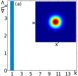
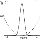
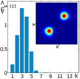
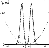
Figure 1: BEC-BEC regime without (upper row) and with (lower row) coupling between species. The left column shows the average occupations $\left\langle n_{k}\right\rangle$ of the momenta $k$. Insets are the corresponding SPDMs, spanning a region of $6\mu m\times 6\mu m$. The right column shows the density profiles, with the dashed line being the potential, the solid line being the density obtained from the SPDM and the solid line with circled markers being the one obtained from a semiclassical GPE-GPE simulations. The dash-dotted lines in (d) are the approximate Gaussians located at the minima of the double well potential $V_{NL}(x)=V(x)+g_{AB}N_{B}|\phi_{0}(x)|^{2}|$.

BEC-BEC regime – If the interactions $g_{E,S}$ are small and $g_{ES}$ vanishes it is sufficient to use only a few modes to describe both species. Indeed, if the intra-species coupling constants vanish as well, the single particle density matrix (SPDM), defined as $\rho_{E}(x,x^{\prime})=\sum_{k,k^{\prime}}\phi_{k}(x)\phi_{k^{\prime}}(x^{\prime})\left\langle\right.\!\!a_{k}^{\dagger}a_{k^{\prime}}\!\!\left.\right\rangle$ and similarly for $\rho_{S}(x,x^{\prime})$, is simply a Gaussian of width $\alpha=\sqrt{\hbar/M\omega}$. For weak interactions the atoms still mainly occupy the lowest energy eigenfunction ( $N_{1}^{E,S}\approx N^{E,S}$) and a Gaussian approximation to the eigenstates will be good. Assuming spatial overlap between both components, the energy of the ground state $\Psi_{0}$ can then be found as

$$E^{\mathrm{hom}}= (N_{E}+N_{S})\frac{\hbar\omega}{2}+\frac{g_{E}}{2\sqrt{2\pi}\alpha}N_{E}(N_{E}-1)$$

$$+\frac{g_{S}}{2\sqrt{2\pi}\alpha}N_{S}(N_{S}-1)+\frac{g_{ES}}{\sqrt{2\pi}\alpha}N_{E}N_{S},$$ (8)

where we have used that $V_{0000}^{E,S}=g_{E,S}/2\sqrt{2\pi}\alpha$. If the two species phase separate, one of them, say $E$, will stay in the center of the trap, approximately with a Gaussian shape of width $\alpha_{E}$. A single Gaussian mode then suffices in the expansion of the field operator of the environment. The system component will approximately assume a profile formed by two Gaussians of width $\frac{\alpha_{S}}{2}$ (see Fig. 1(d)), which we call $\varphi_{0}^{DW}$. In the harmonic oscillator basis the expansion of this state requires a larger number of modes, however, if we use the approximation of $\varphi_{0}^{DW}$ as two displaced Gaussians in a potential of frequency $\omega^{\prime}$, we find the energy of this state as

$$E^{\mathrm{inh}}= N_{E}\frac{\hbar\omega}{2}+\frac{g_{E}}{2\sqrt{2\pi}\alpha_{E}}N_{E}(N_{E}-1)$$

$$+N_{S}\frac{\hbar\omega^{\prime}}{2}+\frac{g_{S}}{2\sqrt{2\pi}\alpha_{S}}N_{S}(N_{S}-1).$$ (9)

To determine the point at which phase separation happens, we assume that the atoms occupy the same total volume before and after phase separation, $\alpha_{E}+\alpha_{S}=\alpha$ Ao:98 , and minimize the energy with respect to $\alpha_{E}$ and $\alpha_{S}$. This gives $\alpha_{E}=\frac{\alpha}{1+k}$ and $\alpha_{S}=\frac{\alpha}{1+k^{-1}}$, with $k=\sqrt{\frac{g_{S}}{g_{E}}\frac{N_{S}(N_{S}-1)}{N_{E}(N_{E}-1)}}$. Subtracting both energies we obtain the phase separation criterion

$$g_{ES}N_{E}N_{S}>\sqrt{g_{E}g_{S}}\sqrt{N_{E}(N_{E}-1)N_{S}(N_{S}-1)},$$ (10)

where we have assumed that the change in kinetic energy $\hbar N_{S}(\omega^{\prime}-\omega)$ is negligible compared to the overall change in interaction energies (we justify this assumption below). This criterion resembles the semiclassical one for large particle numbers, $N_{E,S}(N_{E,S}-1)\approx N_{E,S}^{2}$ Ho:96 ; Ao:98 . Note that it predicts phase separation for any nonzero value of $g_{ES}$ if one of the components consists only of a single particle. If we expand $\varphi_{0}^{DW}$ in terms of the eigenfunctions of the harmonic potential $\varphi_{0}^{DW}=\sum\left\langle\varphi_{0}^{DW}|\phi_{k}\right\rangle\phi_{k}$, we can see that the process of phase separation coincides with the occupation of more and more orbitals in the harmonics basis. Consequently, the phase separated species will be the one with the higher coupling constant and the smaller number of atoms and for simplicity we therefore assume in the following $g_{S}>g_{E}$ and $N_{E}\gg N_{S}$. This assumption also makes numerical calculations possible, since the shape of the environment component does not change substantially after phase separation ($\alpha_{E}\approx\alpha$) and it can correspondingly be described only considering a single mode.

Let us consider an example using atoms of the mass of ⁸⁷Rb in a trap of frequencies $\omega=2\pi\cdot 400$Hz and $\omega_{\perp}=100\omega$. We (exemplary) choose the scattering lengths to be $a_{E}=a_{0}/10$ and $a_{S}=10a_{0}$, where $a_{0}$ is the Bohr radius. The environment consists of $N_{E}=300$ particles and the immersed component of $N_{S}=4$, giving $g_{E}=10^{-9}\hbar\omega$ and $g_{S}=1.01\times 10^{-7}\hbar\omega$. In all calculations we use $n_{S}=14$ and $n_{E}=1$ (as justified above). In the upper row in Fig. 1 we show the situation where the different species do not interact ($g_{ES}=0$), while in the bottom row $g_{ES}=\frac{g_{S}}{2}$, which is deep inside the phase separated regime. As expected, for $g_{ES}=0$ the SPDM of both species is Gaussian, as shown in the inset of Fig. 1(a) for the system component. The energy of the sample in this case is given by eq. (Quantum gas mixtures in different correlation regimes) as $E^{\mathrm{hom}}=187.0\,\hbar\omega$. Correspondingly, the average occupation for the system component $\langle n_{k}\rangle=\langle b_{k}^{\dagger}b_{k}\rangle$, represented in Fig. 1(a), shows that mainly one momentum component is occupied, because the coupling constant is very small. For bigger $g_{S}$ higher lying momenta will start gaining occupation, however the system will still form a BEC as the occupation of the lowest momentum component is of the order of $N_{S}$. As long as the sample is in this limit no phase separation occurs. Fig. 1(b) shows the density of the system component obtained from the SPDM (solid line) coinciding with the semiclassical calculation using two coupled GPE (solid line with circled markers).

If $g_{ES}=\frac{g_{S}}{2}$ (lower row in Fig. 1) the energy for a phase separated state is much smaller than that for a mixed phase, $E^{\mathrm{inh}}=191.0\,\hbar\omega<E^{\mathrm{hom}}=230.8\,\hbar\omega$ and also corresponds approximately to the one calculated numerically of $E=195.0\,\hbar\omega$. Accordingly, the SPDM in this situation (see inset of Fig. 1(c)) shows that phase separation has occurred and an occupation of higher momentum modes is found (see Fig. 1(c)). The densities calculated from the SPDM and obtained from the numerical solution of the coupled GPE shows again good agreement (see Fig. 1(d)). The Gaussian functions used to calculate the energy given by eq. (Quantum gas mixtures in different correlation regimes) are located at the minima of the double well potential $V_{NL}(x)=V(x)+g_{ES}N_{S}|\phi_{0}(x)|^{2}|$, which are given by $d=\pm\alpha\sqrt{\beta}$, with $\beta=\ln\left(2g_{ES}N_{S}/\alpha^{3}M\sqrt{\pi}\omega^{2}\right)$. The local trapping frequency can then be approximated as $\omega^{\prime}=\sqrt{2}\omega\beta$, leading to a width of the Gaussians of $\alpha^{\prime}=\sqrt{\hbar/M\omega^{\prime}}$. We can now estimate the increase in the kinetic energy due to phase separation as $\hbar N_{S}\omega(1-\sqrt{2}\beta)$, which has to be compared to the change in the interaction energies ($g_{ES}N_{E}N_{S}$ and $\sqrt{g_{E}g_{S}}\sqrt{N_{E}(N_{E}-1)N_{S}(N_{S}-1)}$). Since the latter is quadratic in the number of particles it is generally much larger except for systems with very small coupling constants and number of atoms.

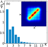
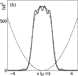
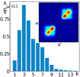
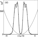
Figure 2: BEC-TG regime without (upper row) and with (lower row) coupling between species. Panel lay-out as in Fig. 1. The semiclassical profiles are obtained using the mean field equations described in the text.

BEC-TG regime – We now consider the case where the system component is in the Tonks-Girardeau regime. In Fig. 2 we show the same quantities as before, but now for $N_{E}=40$, $a_{E}=a_{0}$ and $a_{S}=500a_{0}$, which gives a Lieb-Liniger parameter of $\gamma=2g_{S}ML/\hbar^{2}N_{S}=4.5$ Lieb:63 , where $L$ is the size of the cloud. This corresponds to the system component being in the Tonks-Girardeau regime and we find the interaction coefficients to be $g_{E}=10^{-8}\hbar\omega$ and $g_{S}=9.6\times 10^{-5}\hbar\omega$. As expected, for no inter-species interaction the SPDM and the momentum distribution for the system component resemble that of a TG gas (Fig. 2 (a)). The density profiles calculated from the microscopic and the semiclassical approach (see below and Fig. 2 (b)) show again good agreement. Though the phase separation criterion of eq. (10) is only approximately valid in this regime, due to the deviations from the Gaussian shapes for the individual components, it is still useful away from the precise border transition point. The lower row of Fig. 2 shows the situation for $g_{ES}=0.05g_{S}$, where phase separation is clearly visible in the SPDM and the momentum distribution shows a shift of the momenta due to the density resembling a higher excited state.

To compare the above results with a mean-field model in the semiclassical limit, we chose to model the strongly correlated system component using a quintic non-linearity in the field equation Kolomeisky:00 . While one has to be aware that this approach for a TG gas does not describe the coherence properties correctly Girardeau:00 , it is known to give a good approximation to the exact density in the single component case. This equation is then coupled to a GPE for the BEC component, giving

$$i\hbar\dot{\psi}_{S}= -\frac{\hbar^{2}}{2m}\psi_{S}^{{}^{\prime\prime}}+\left[V(x)+\tilde{g}_{S}|\psi_{S}|^{4}+g_{ES}|\psi_{E}|^{p}\right]\psi_{S}$$ (11a)

$$i\hbar\dot{\psi}_{E}= -\frac{\hbar^{2}}{2m}\psi_{E}^{{}^{\prime\prime}}+\left[V(x)+g_{E}|\psi_{E}|^{2}+g_{ES}|\psi_{S}|^{p}\right]\psi_{E},$$ (11b)

where $\tilde{g}_{S}=\frac{\left(\pi\hbar\right)^{2}}{2M}$. If the interactions between both components are small, i.e. $\gamma^{\prime}=2g_{ES}ML/\hbar^{2}N_{S}<1$, the exponent on the non-linear coupling term is given by $p=2$ and in the opposite limit by $p=4$. For the parameters used in Fig. 2 we find $\gamma^{\prime}=0.22$ and the numerical solution of eqs. (11) show good agreement with the microscopically calculated density (see Fig. 2(c)). Calculations for increased values of $g_{ES}$, which require $p=4$ also show good agreement, but are not shown here.

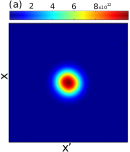
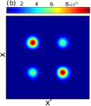
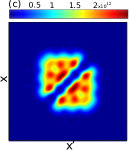
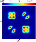
Figure 3: Pair correlation functions $g^{(2)}(x,x^{\prime})$ spanning an area of $6\mu m\times 6\mu m$. The top row shows the BEC-BEC cases using the same parameters as in Fig. 1 for the situation (a) without and (b) with coupling between species. The lower row shows the BEC-GP regime analogous to the situation in Fig. 2 for the situation (c) without and (d) with coupling between the species.

Let us finally discuss the pair correlation functions $g^{(2)}(x,x^{\prime})=\langle\hat{\Psi}^{\dagger}(x)\hat{\Psi}^{\dagger}(x^{\prime})\hat{\Psi}(x^{\prime})\hat{\Psi}(x)\rangle$, with $\hat{\Psi}(x)$ being the field operator, using again the microscopic model. These correlations give the probability of finding an atom at position $x$ once another atom has been measured at $x^{\prime}$. The BEC-BEC case with no interaction between species (corresponding to the upper row of Fig. 1) is shown in Fig. 3(a) and the expected Gaussian profile is obtained. In the phase separation regime (see Fig. 3(b)) we find that the two approximately Gaussian parts of the density profile of the system (shown in the lower row in Fig. 1) are highly correlated . For the BEC-TG case with no inter-species interaction (corresponding to the upper row in Fig. 2), as shown in Fig. 3(c), we recover the well-known hard-sphere behaviour that no two atoms can be found at the same point in space, which persists in the phase separated limit for the individual peaks (see Fig. 3(d)). The correlations between the two peaks are also still visible, however they show a more complicated structure due to the inter-species interaction.

In conclusion, we have presented a microscopic and a semiclassical model to describe a two-component Bose gas at ultralow temperatures in the one-dimensional limit. Since we allow for one component to be in any correlation regime, our work generalises the known models for interpenetrating Bose-Einstein condensates to include a significantly larger group of systems, which are currently about the become experimentally available.

From our microscopic model we have, as a first example, derived a criterion for phase separation, which extends the well-known mean field result to the mesoscopic limit. We have also presented a semiclassical description of a mixture of ultracold bosons when one of them is highly interacting, and found that the nonlinear coupling term between the species depends on the interaction strength. Finally, we have shown that even when the atoms are phase separated, they are still strongly correlated among themselves. Interesting questions that can be approached with this model include the study of quantum correlations between a system and an environment in fundamental settings as well as using one component (one matter wave) to engineer the state of the second matter wave.

- (1) R. Côté et al. Phys. Rev. Lett. 89, 093001 (2002); M. Bruderer et al. Phys. Rev. A 76, 011605R (2007); J. Goold et al. Ibid 81, 041601(R) (2010); J. Goold et al. Ibid 84, 063632 (2011).
- (2) C. Zipkes et al. Nature 464, 388 (2010); S Schmid et al. Phys. Rev. Lett. 105, 133202 (2010); S. Will, et al. Ibid 106, 115305 (2010).
- (3) H. Doerk, Z. Idziaszek, and T. Calarco, Phys. Rev. A 81, 012708 (2010).
- (4) C.J. Myatt et al. Phys. Rev. Lett. 78, 586 (1997); D.M. Stamper-Kurn et al. Ibid 80, 2027 (1998); S.R. Granade et al. Ibid 88, 120405 (2002); F. Schreck et al. Ibid 87, 080403 (2001); A.G. Truscott et al. Science 291, 2570 (2001).
- (5) C.K. Law et al. Phys. Rev. Lett. 79, 3105 (1997); E.V. Goldstein and P. Meystre, Phys. Rev. A 55, 2935 (1997); B. D. Esry and Chris H. Greene, ibid 57, 1265 (1998).
- (6) T.-L. Ho and V. B. Shenoy, Phys. Rev. Lett. 77, 3276 (1996); B.D. Esry et al. Ibid 78, 3594 (1997).
- (7) Th. Busch et al. Phys. Rev. A 56, 2978 (1997).
- (8) P. Ao and T. Chui, Phys. Rev. A 58, 4836 (1998).
- (9) M. Girardeau, J. Math. Phys. 1, 516 (1960).
- (10) M. Girardeau et al. Phys. Rev. A 63, 033601 (2001).
- (11) B. Paredes et al. Nature 429, 277 (2004); T. Kinoshita et al. Science 305, 1125 (2004).
- (12) J. Goold et al. New J. Phys. 12, 093041 (2010).
- (13) F. Deuretzbacher et al. Phys. Rev. A 75, 013614 (2007).
- (14) E.B. Kolomeisky et al. Phys. Rev. Lett. 85, 1146 (2000).
- (15) M. Olshanii, Phys. Rev. Lett. 81, 938 (1998).
- (16) E. Lieb and W. Liniger, Phys. Rev. 130, 1605 (1963); E. Lieb, ibid. 130, 1616 (1963).
- (17) M.D. Girardeau and E.M. Wright, Phys. Rev. Lett. 84, 5239 (2000).