NEW ATLAS9 AND MARCS MODEL ATMOSPHERE GRIDS FOR THE APACHE POINT OBSERVATORY GALACTIC EVOLUTION EXPERIMENT (APOGEE)

Abstract

We present a new grid of model photospheres for the SDSS-III/APOGEE survey of stellar populations of the Galaxy, calculated using the ATLAS9 and MARCS codes. New opacity distribution functions were generated to calculate ATLAS9 model photospheres. MARCS models were calculated based on opacity sampling techniques. The metallicity ([M/H]) spans from $-$5 to 1.5 for ATLAS and $-$2.5 to 0.5 for MARCS models. There are three main differences with respect to previous ATLAS9 model grids: a new corrected H₂O linelist, a wide range of carbon ([C/M]) and $\alpha$ element [$\alpha$/M] variations, and solar reference abundances from Asplund et al. (2005). The added range of varying carbon and $\alpha$ element abundances also extends the previously calculated MARCS model grids. Altogether 1980 chemical compositions were used for the ATLAS9 grid, and 175 for the MARCS grid. Over 808 thousand ATLAS9 models were computed spanning temperatures from 3500 K to 30000 K and log $g$ from 0 to 5, where larger temperatures only have high gravities. The MARCS models span from 3500 K to 5500 K, and log $g$ from 0 to 5. All model atmospheres are publically available online.

1. Introduction

The Apache Point Observatory Galactic Evolution Experiment (APOGEE; Allende Prieto et al. 2008) is a large-scale, near-infrared, high-resolution spectroscopic survey of Galactic stars, and it is one of the four experiments in the Sloan Digital Sky Survey-III (SDSS-III; Eisenstein et al. 2011; Gunn et al. 2006, Aihara et al. 2011). APOGEE will obtain high S/N, R$\sim$22,500 spectra for 100,000 stars in the Milky Way Galaxy, for which accurate chemical abundances, radial velocities, and physical parameters will be determined. APOGEE data will shed new light on the formation of the Milky Way, as well as its chemical and dynamical evolution. To achieve its science goals, APOGEE needs to determine abundances for about 15 elements to an accuracy of 0.1 dex. To attain this precision, a large model photosphere database with up-to-date solar abundances is required. We chose to build the majority of APOGEE’s model photosphere database on ATLAS9 and MARCS calculations.

ATLAS (Kurucz, 1979) is widely used as a universal LTE 1$-$D plane-parallel atmosphere modeling code, which is freely available from Robert Kurucz’s website. ATLAS9 (Kurucz, 1993) handles the line opacity with the opacity distribution functions (ODF), which greatly simplifies and reduces the computation time (Strom $\&$ Kurucz, 1966; Kurucz, 2005; Castelli, 2005). ATLAS uses the mixing-length scheme for convective energy transport. It consists in pretabulating the line opacity as function of temperature and gas pressure in a given number of wavelength intervals which cover the whole wavelength range from far ultraviolet to far infrared. For computational reasons, in each interval the line opacities are rearranged according to strength rather than wavelength. For each selected metallicity and microturbulent velocity, an opacity distribution function table has to be computed. While the computation of the ODFs is very time consuming, extensive grids of model atmospheres and spectrophotometric energy distributions can be computed in a short time once the required ODF tables are available.

ATLAS12 (Kurucz, 2005; Castelli, 2005) uses the opacity sampling method (OS) to calculate the opacity at 30,000 points. The high resolution synthetic spectrum at a selected resolution can then be obtained by running SYNTHE (Kurucz $\&$ Avrett, 1981). More recently, Lester $\&$ Neilson (2008) have developed SATLAS__ODF and SATLAS__OS, the spherical version of both ATLAS9 and ATLAS12, respectively. No extensive grids of models have been published up to now, neither with ATLAS12, nor with any of the two versions of SATLAS.

Instead, extensive grids of ATLAS9 ODF model atmospheres for several metallicities were calculated by Castelli $\&$ Kurucz (2003). These grids are based on solar (or scaled solar) abundances from Grevesse $\&$ Sauval (1998). Recently, Kirby (2011) provided a new ATLAS9 grid, but he used abundances from Anders $\&$ Grevesse (1989). The calculations presented in this paper are based on the more recent solar composition from Asplund et al. (2005). This updated abundance table required new ODFs and Rosseland mean opacity calculations as well. Abundances from Asplund et al. (2005) were chosen instead of those from newer studies (Asplund et al., 2009) to match the composition of the MARCS models described below, and those available from the MARCS website.

The MARCS model atmospheres (Gustafsson et al., 1975; Plez et al., 1992; Gustafsson et al., 2008) were developed and have been evolving in close connection with applications primarily to spectroscopic analyses of a wide range of late type stars with different properties. The models are one-dimensional plane-parallel or spherical, and computed in LTE assuming the mixing-length scheme for convective energy transport, as formulated by Henyey et al. (1965). For luminous stars (giants), where the geometric depth of the photosphere is a non-negligible fraction of the stellar radius, the effects of the radial dilution of the energy transport and the depth-varying gravitational field is taken into account. Initially, spectral line opacities were economically treated by the ODF approximation, but later the more flexible and realistic opacity sampling scheme has been adopted. In the OS scheme, line opacities are directly tabulated for a large number of wavelength points (10⁵) as a function of temperature and pressure.

The shift in the MARCS code from using ODFs to the OS scheme avoided the sometimes unrealistic assumption that the line opacities of certain relative strengths within each ODF wavelength interval overlap in wavelength irrespective of depth in the stellar atmosphere. This assumption was found to lead to systematically erroneous models, in particular when plolyatomic molecules add important opacities to surface layers (Ekberg et al., 1986). The current version of the MARCS code used for the present project and for the more extensive MARCS model atmosphere data base was presented and described in detail by Gustafsson et al. (2008). The model atmospheres presented in this paper adds large variaty in [C/M] and [$\alpha$/M] abundances to the already existing grids by covering these abundances systematically from -1 to +1 for each metallicity.

Our main purpose is to update the previous ATLAS9 grid and publish new MARCS models to provide a large composition range to use in the APOGEE survey and future precise abundance analysis projects. These new ATLAS models were calculated with a corrected H₂O linelist. The abundances used for the MARCS models presented in this paper are from Grevesse et al. (2007), which are nearly identical to Asplund et al. (2005); the only significant difference is an abundance of scandium 0.12 dex higher than in Asplund et al. (2005). The range of stellar parameters (T_eff, log $g$ and [M/H]) spanned by the models covers most stellar types found in the Milky Way.

This paper is organized as follows. In Section 2 we describe the parameter range of our ODFs and model atmospheres and give details of the calculation method of ATLAS9 we implemented. Section 3 contains the parameter range and calculation procedure for MARCS models. In Section 4 we compare MARCS and ATLAS9 models with Castelli $\&$ Kurucz (2003), and illustrate how different C and $\alpha$ contents affect the atmosphere. Section 5 contains the conclusions. The grid of ODFs and model atmospheres will be periodically updated in the future and available online.

Figure 1.— The [C/M] or [$\alpha$/M] content as a function of [M/H] of ATLAS9 models (filled circles, Table 1) and MARCS models (open circles, Table 4). Both [C/M] and [$\alpha$/M] changes independently from each other, and the small steps in metallicities give altogether 1980 different compositions for the ATLAS9 models and 175 compositions for the MARCS models. The number of acceptable models may vary for each composition, for details see the ATLAS-APOGEE website (http://www.iac.es/proyecto/ATLAS-APOGEE/). For missing metal-rich compositions of ATLAS9 models see Table 2.

2. ATLAS9 Model Atmospheres

2.1. Parameters

The metallicity ([M/H]) of the grid varies from $-$5 to 1.5 to cover the full range of chemical compositions and scaled to solar abundances. For each of these solar scaled compositions we also vary the [C/M] and [$\alpha$/M] abundances from $-$1.5 to 1 (Figure 1).

ODFs and Rosseland opacity files were calculated with microturbulent velocities v_t = 0, 1, 2, 4, 8 km s^-1, while the model atmospheres were produced only with v_t = 2 km s^-1. The metallicity grids were the same for all effective temperatures, and the range can be seen in Table 1. Some metal-rich compositions with high C but low $\alpha$ content were not calculated due to excessive computation time; these are listed in Table 2. The $\alpha$ elements considered when varying [$\alpha$/M] were the following: O, Ne, Mg, Si, S, Ca, and Ti. The temperature and gravity parameter grid for each composition and spectral type is given in Table 3. The T_eff $-$ log $g$ distribution is plotted in Figure 2. Extreme metal-poor and metal-rich compositions were also included.

Figure 2.— The gravity (log $g$) as a function of effective temperature (T_eff) of ATLAS9 and MARCS models calculated for each composition. Acceptable models are denoted by filled circles, while models not acceptable (and missing) are denoted by open circles for the solar composition. Models with C/O $>$ 1.7 and T${}_{\rm eff}<4000$ K are not published (see Section 4.2).

All the ATLAS codes use atomic and molecular linelists made available by Kurucz on a series of CDROM (Kurucz, 1990). They can now be found at the Kurucz website. The molecular line lists for TiO and H₂O were provided by Schwenke (1998) and Partridge $\&$ Schwenke (1997), respectively, and reformatted by Kurucz in ATLAS format. These are also available for download at the Kurucz website. For these models, we used the same linelists as Castelli $\&$ Kurucz (2003), except for H₂O, for which a new Kurucz release of the Partridge $\&$ Schwenke (1997) data was adopted.

The solar reference abundance table was adopted from Asplund et al. (2005). Convection was turned on with the mixing length parameter set to $l/H_{p}=1.25$, but the convective overshooting was turned off. All the models have the same 72 layers from log $\tau_{Ross}$ = $-$6.875 to 2, where the step is log $\tau_{Ross}$ = 0.125. These parameters remained the same as Castelli $\&$ Kurucz (2003) for easy comparison.

All computations were performed on the Diodo cluster at the Instituto Astrofisico de Canarias. Diodo consists of 1 master node and 19 compute nodes, for a total of 80 cores and 256 GB of RAM, communicating through two independent Gigabit Ethernet networks. 16 of the compute nodes host 2 Intel Xeon 3.20 GHz EM64T processors each, with 4 GB of RAM (2GB per core); the remaining 3 compute nodes host each 16 Intel Xeon (E7340) 2.40 GHz EM64T processors, with 64 GB of RAM (4GB per core). On this cluster, about 3 months of computer time was required for ODF and model atmosphere calculations, using all 80 processors.

2.2. Calculation Method

Two separate scripts were developed, one for the ODF and Rosseland opacity calculations, and one for the ATLAS9 calculations. The ODF and Rosseland opacity calculations followed exactly the procedure described by Castelli $\&$ Kurucz (2003), and Castelli (2005) using the DFSYNTHE code for the ODF, KAPPA9 code for the Rosseland opacity, and ATLAS9 for the model atmopshere calculations (Sbordone, 2004, 2005). These codes were compiled in Linux with the Intel Fortran compiler version 11.1.

Table 1Abundance Parameters of ATLAS9 models

	Min	Max	Step
$[$M/H$]$	$-$5	$-$3.5	0.5
$[$C/M$]$	$-$1	1	0.5
$[\alpha$/M$]$	$-$1	1	0.5
$[$M/H$]$	$-$3	0.5	0.25
$[$C/M$]$	$-$1.5	1	0.25
$[\alpha$/M$]$	$-$1.5	1	0.25
$[$M/H$]$	1	1.5	0.5
$[$C/M$]$	$-$1.5	1	0.5
$[\alpha$/M$]$	$-$1.5	1	0.5

Table 2Missing compositions of ATLAS9 models

[M/H]	[C/M]	[$\alpha$/M]
1	1	$-$1.5
1	1	$-$1
1.5	0.5	$-$1.5
1.5	1	$-$1.5
1.5	1	$-$1
1.5	1	$-$0.5
1.5	1	0

Table 3Model Atmosphere Parameters of ATLAS9 models

Spectral Type	$T_{\rm eff}$	$T_{\rm eff}$	$T_{\rm eff}$	log $g$	log $g$	log $g$
	min	max	step	min	max	step
M, N, R, K, G	3500	6000	250	0	5	0.5
F	6250	8000	250	1	5	0.5
A	8250	12000	250	2	5	0.5
B	12500	20000	500	3	5	0.5
B, O	21000	30000	1000	4	5	0.5

Our algorithm sets up the initial starting models from the grid provided by Castelli $\&$ Kurucz (2003). The algorithm chooses the model that has the closest composition, effective temperature, and log $g$ to the desired output, and an initial ATLAS9 model is calculated. The result must be checked to see whether the output model satisfies the convergence parameters provided by the user for each layer in the model atmosphere. These parameters were set to 1$\%$ for the flux or 10$\%$ for the flux derivative errors after 30 iterations in each run, as recommended in the ATLAS cookbook. A model is considered converged if the convergence parameters satisfy these criteria in all depths.

We then determined that an atmospheric model is acceptable if one of the following criteria is satisfied: 1. the model has converged through the whole atmosphere, 2. no more than 1 non-converged layer exists between log $\tau_{\rm Ross}=-4$ and log $\tau_{\rm Ross}=1$. The model is allowed to have other non-converged layers for log $\tau_{\rm Ross}<-4$. A model was considered unacceptable in all other cases. We used only log $\tau_{\rm Ross}>=-4$ to log $\tau_{\rm Ross}=1$ to check the convergence, because most of the lines in the optical and H band form in this region. In case the output was not acceptable, we restarted the calculation using more iterations. In case of a run with unacceptable output, we selected a starting model that had a different log $g$ from the initial starting model and used it to restart the calculation. Then the previously described convergence test was performed and more restarts were done if it was necessary. If the output remained unacceptable, the effective temperature of the output model was changed by 10, 50, and 100 K. If the output of any of these runs was acceptable, then it was used as an input model to calculate the atmosphere with the original effective temperature.

To test our model atmospheres, we replicated the Rosseland opacity calculations by Castelli $\&$ Kurucz (2003). For this we used Castelli’s scripts without any modification to calculate the ODF, and Rosseland opacities for the Grevesse $\&$ Sauval (1998) abundances. These calculations concluded in perfect agreement within numerical precision. We then attempted to reproduce model atmospheres with the same parameters found on Castelli’s website with our scripts using the ODFs and Rosseland opacity files generated with Grevesse $\&$ Sauval (1998) abundances. This test also concluded with near perfect agreement with only 0.1$-$0.2 K maximum differences coming from the different version of compilers used.

3. MARCS Model Atmospheres

3.1. Parameters

Models were computed for seven overall metallicities, [M/H] from $-$2.5 to 0.5, with a step size of 0.5 dex. For each of these seven overall [M/H] mixtures, 25 combinations of modified carbon and $\alpha$ element abundances were adopted: The modifications to the logarithmic C and $\alpha$ abundances are $-$1, $-$0.5, 0, 0.5, and 1  dex. This format resulted in a total of 175 subgrids with unique chemical compositions (Table 4). The $\alpha$ elements in MARCS are O, Ne, Mg, Si, S, Ar, Ca, and Ti. This composition scheme is exactly the same as the previous models found on the MARCS website. The systematic $\alpha$ abundance changes were chosen to overlap the scheme (Section 2.1) used in the ATLAS9 model calculations.

Table 4Abundance Parameters of MARCS models

	Min	Max	Step
$[$M/H$]$	$-$2.5	0.5	0.5
$[$C/M$]$	$-$1	1	0.5
$[\alpha$/M$]$	$-$1	1	0.5

Table 5Model Atmosphere Parameters of MARCS models

Spectral Type	$T_{\rm eff}$	$T_{\rm eff}$	$T_{\rm eff}$	log $g$	log $g$	log $g$
	min	max	step	min	max	step
M, N, R, K	3500	4000	100	0	3	0.5
K, G	4250	5500	250	0	3	0.5
M, N, R, K	3500	4000	100	3.5	5	0.5
K, G	4250	5500	250	3.5	5	0.5

For each of these abundance subgrids, models with 12 values of effective temperature from 3500 to 5500 K and 11 values of logarithmic surface gravities from 0 to 5 were computed (see Figure 2 and Table 5). Models with logarithmic surface gravities lower than 3.5 (giants) were computed in spherical geometry and with a microturbulence parameter of 2 km s^-1, while the remaining (dwarf) models adopted v_t = 1 km s^-1 and plane-parallel geometry. In the end, 86% of the 23,140 models converged satisfactorily. Convergence was particularly poor for cool dwarfs that are simultaneously $\alpha$ rich and carbon poor.

Details about the atomic and molecular line lists used by the MARCS code are given by Gustafsson et al. (2008). In a number of instances, they are different from those used by the ATLAS code, as for H₂O (Barber et al., 2006), and TiO (Plez, 1998).

3.2. Calculation Method

Similarly to the ATLAS9 ODF calculations, a new metallicity MARCS subgrid is started with the summation of an OS table of atomic line opacities for the relevant abundance mixture and microturbulence parameter. Since line opacity data is needed for many atoms and first ions, it saves time to add the opacities of the individual species into one file before a set of models is computed. This file contains a table with over 10⁵ wavelength points with line opacities relevant to the equation of state for 306 combinations of temperature and damping pressure $P_{6}$. The damping pressure is used as a proxy for the pressure that broadens metal lines by collisions with neutral atoms in cool stars. $P_{6}$ is the pressure of HI with the addition of the polarizability corrected pressures of neutral helium and H₂ (see Eq. 33 of Gustafsson et al. 2008). For each molecule, in contrast, the line opacities are given in one table for the same wavelength set, but as a function of temperature and microturbulence parameter.

The method used for the MARCS model calculations is described in detail in Gustafsson et al. (2008). They start with the generation of a simplified starting model assuming a grey opacity. Physical parameters and their derivatives are computed and the model structure is iterated in a multidimensional Newton-Raphson scheme until the flux through each depth layer corresponds to the prescribed effective temperature. The models usually converged after 4 to 8 iterations; convergence also requires that the maximum temperature correction in any depth point is below 1.5 K during two consecutive iterations. Occasionally convergence takes longer, and some models do not converge at all. A converged model with similar model parameters is then identified as a new starting model. This approach is often successful, but some models do not converge, which leaves vacancies in the model grid.

4. Discussion

Changes in the chemical composition can have a number of effects on the calculated atmospheres. These effects are mainly related to either changes in opacity or changes in the equation of state. The main effect of an increased line opacity in late-type stars is either cooling or warming (depending on the opacity and its wavelength dependence) of the outer layers and also back-warming of the innermost ones (Gustafsson et al., 1975). Changes in the equation of state are mainly variations in the mean molecular weight for abundant elements, changes in the number of free electrons for elements that are important electron donors, or other more intricate changes related to chemical equilibrium through molecule formation. In the next two sections, we give examples of MARCS and ATLAS9 models from our grid, and illustrate briefly the changes in the model atmospheres related to large changes in C and $\alpha$ elements.

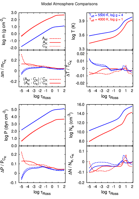
Figure 3.— Examples of ATLAS9 and MARCS model atmospheres with T_eff = 4000 K and log $g$ = 1 (red line) and T_eff = 5500 K and log $g$ = 4 (blue line). The model from the APOGEE grid is denoted by a solid line, the corresponding ATLAS9 model from Castelli $\&$ Kurucz (2003) is denoted by a dotted line, the MARCS model is denoted by dashed line. The panels show the mass column ($m$), temperature ($T$), gas pressure ($P$), electron number density ($N_{\rm e}$) as a function of the logarithm of optical depth (log $\tau$), and the relative difference between the ATLAS9 (A_K), MARCS (A_M) calculations presented in this paper and Castelli $\&$ Kurucz (2003) (C_K).

4.1. Comparing our MARCS and ATLAS9 models to the Castelli-Kurucz grid

Figure 3 illustrates examples of the atmospheric structures for two models with solar composition, one for $T_{\rm eff}=4000$ K and log $g=1$ (red line) and the other for $T_{\rm eff}=5500$ K and log $g=4$ (blue line). There are four double panels showing the parameter dependence with Rosseland optical depth of the mass column (top-left panel), temperature (top-right), gas pressure (bottom-left) and electron number density (bottom-right). The dashed, solid, and dotted lines correspond to the new APOGEE MARCS, APOGEE Kurucz, and earlier (NEWODF) Castelli-Kurucz models (Castelli $\&$ Kurucz, 2003), respectively. While the APOGEE Kurucz and MARCS models share essentially the same chemical composition (Asplund et al., 2005; Grevesse et al., 2007), the Castelli-Kurucz models use the solar mixture given by Grevesse $\&$ Sauval (1998).

For both the cooler (red line) and the warmer model (blue line), we see good agreement between the MARCS and the ATLAS9 models presented in this paper. The new MARCS and ATLAS9 models show good agreement, the differences are modest, less than 1 percent, for the thermal structure, and less than 2$-$3 percent for the gas pressure and the electron density in the layers where weak spectral lines and continuum form ($\tau>$ 0.01). These small differences are most likely related to the different equation of state implemented in the two codes, and can also be due to the fact that ATLAS9 uses the ODF method, while MARCS uses the OS method. The differences between the two increase at temperatures lower than 4000 K due to the different H₂0 and TiO linelists used in the calculations. More importantly, larger differences are present in the gas pressure and electron density in the ATLAS9 models compared to the Castelli-Kurucz ones for the cooler models. These differences must be related to the updated solar chemical composition, as the Castelli-Kurucz models are also computed with a corrected H₂O linelist. The most significant change in the solar composition corresponds to the reduction in oxygen, nitrogen and carbon abundances, all of which decrease in the update. This causes a reduction in the Rosseland opacity at a given temperature and gas pressure. The decreased Rosseland opacity leads to a subsequent increase in the total pressure, which is only partially compensated by a reduction in the electron density.

Gustafsson et al. (2008) present some further comparisons between MARCS models and ATLAS9 models of Castelli $\&$ Kurucz (2003). Other comparisons between MARCS, ATLAS9, and PHOENIX model atmospheres and spectra were discussed by Plez (2011).

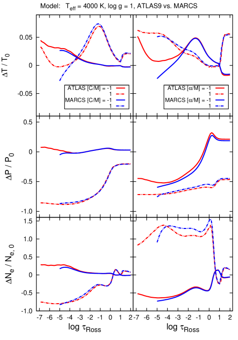
Figure 4.— Examples of how different [C/M] and [$\alpha$/M] content changes the temperature profile in the ATLAS9 and MARCS atmospheres for T_eff = 4000 K, log $g$ = 1. This figure shows the temperature ($T$), gas pressure ($P$), electron number density ($N_{\rm e}$) and the relative difference (where 0.5 corresponds to 50%, 1 corresponds to 100%) of these parameters between [C/M]=[$\alpha$/M] = 0 and [C/M]=[$\alpha$/M] = $-$1, and 1 as a function of optical depth (log $\tau$). The symbols $T_{0}$, $P_{0}$, $N_{e,0}$ correspond to [C/M]=[$\alpha$/M] = 0.

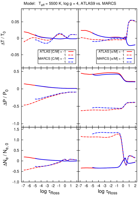
Figure 5.— Examples of how different [C/M] and [$\alpha$/M] content changes the temperature profile in the ATLAS9 and MARCS atmospheres for T_eff = 5500 K, log $g$ = 4. For more details see the caption of Figure 6.

4.2. Changes in model structures related to chemical composition

Figures 4 and 5 illustrate the changes in the model structures in response to changes in chemical composition. The left-hand panels of Figure 4 (T${}_{\rm eff}=4000$ K model) and 5 (T${}_{\rm eff}=5500$ K) show the relative changes associated with variations of the carbon abundance from solar proportions. The ATLAS9 model for the warmer temperature has v_t = 2 km s^-1, while the MARCS model has v_t = 1 km s^-1, but this difference does not affect the model structures significantly. The relative variations found are very similar for MARCS and ATLAS9, except in the outermost layers of the atmosphere. The changes in the thermal structure are modest and show a behavior symmetric to that found for oxygen, which strongly suggests that CO formation is the driver of the variation. CO is the most tightly bound molecule and consumes almost all of the free atoms of either carbon or oxygen, whichever is less abundant, leaving the majority species (C I or O I) to form other molecules. If oxygen dominates, it produces a ”normal star” (if cool, an M star), otherwise carbon is free to form many molecules with high opacities, making carbon stars with very different spectra. At T${}_{\rm eff}=5500$ K, CO formation is low, thus this molecule does not affect the chemical equilibrium contrary to what is seen in the cooler atmospheres.

The right-hand panels show changes for the same model parameters and different $\alpha$-element abundances. Large changes are visible for both models in the pressure and electron numbers. The significant differences in the pressure compared to the cooler model are due to the increased gravity. Increasing the abundance of $\alpha$ elements reduces pressure (despite the fact that electron pressure increases), because the electrons of the other main electron contributors change the continuum opacity. The $\alpha$ elements that contribute most to the total number of electrons in the ATLAS9 models are shown in Figure 6. For the T${}_{\rm eff}=4000$ K, log $g=1$ model, the main electron contributors are Ca, Mg, Na, and Al in the outer layers and Mg, Si and Fe in the deeper layers. For the warmer models, this changes significantly, as more Fe and H is ionized, the overall number of electrons increases and the main electron contributors become Mg, Si, and Fe through most of the atmospheres.

Internal tests showed that polyatomic carbon molecules (C₂H₂, C3) substantially change the structure of the atmosphere with C/O ratios higher 1.7, if they are included in the linelist. These molecules significantly inflate the atmosphere changing the temperature in the line-forming photospheric layers. Since these molecules were used neither in the ATLAS9, nor in the MARCS calculations, atmospheric structures with C/O $>$ 1.7 and T${}_{\rm eff}<4000$ K are not reliable and thus not published.

Figure 6.— Examples of the largest electron contributors to the total electron numbers in the ATLAS9 atmospheres for [M/H]=[C/M]=[$\alpha$/M] = 0. The figure shows the element electron numbers relative to the total number of electrons for the two models used in previous figures. The T${}_{\rm eff}=5500$ K, log $g=1$ model is plotted in the middle section to show that the electron contributors do not change significantly compared to a model with the same temperature but higher gravity.

5. Conclusions

Most of the ATLAS9 models are fully converged above T_eff = 5000 K. Convergence problems are visible only in the outermost layers for stars with T${}_{\rm eff}<$ 5000 K. The regions affected by convergence issues are limited to log $\tau_{\rm Ross}<-$4. However, these un-converged layers on the top of the atmosphere at low temperatures do not affect most line profiles very significantly, because most lines form deeper in the atmosphere. A little over a million ATLAS9 atmospheres were calculated.

Over 20,000 MARCS fully converged models with ranges in [C/M] and [$\alpha$/M] have been produced. Models are available in spherical and plane-parallel cases. Convergence issues are also present for red dwarf stars, similarly to the ATLAS9 models.

Examples were presented for both ATLAS9 and MARCS models for T${}_{\rm eff}=4000$ K and 5500 K, and compared to the Castelli-Kurucz grid. The new ATLAS9 and MARCS models agree well for all temperatures, while the differences between these calculations and the Castelli-Kurucz grid arise from the updated abundance tables. We briefly illustrated the effects of decreased/increased carbon and $\alpha$ content on the structure of the atmospheres, which are very similar in the MARCS and ATLAS9 models. The response to the carbon content is only different in the outermost layers due to increased CO in the atmosphere. The response to $\alpha$ elements is also almost the same in MARCS and ATLAS9 models. The increased $\alpha-$element content has profound effects in electron numbers and pressure for both the giant and dwarf stars, which is related to the higher number of Mg, Si, and Ca ions. Carbon rich models with C/O $>$ 1.7 and T${}_{\rm eff}<4000$ K are not published here, because polyatomic carbon molecules not included in the linelists here significantly change the temperature structure in the photosphere.

These model grids will be used as the primary database for the pipeline analysing the spectra from the APOGEE survey. The high-resolution model spectra used in the survey’s atmospheric parameters and abundances determination code will be built on the models presented in this paper. Both the ATLAS9 and MARCS models atmospheres will be continuously updated with new compositions as the APOGEE survey progresses. The calculated ODFs, Rosseland opacities available for v_t = 0, 1, 2, 4, 8 km s^-1, and the ATLAS9 model atmosphere files are available for v_t = 2 km s^-1 from the ATLAS-APOGEE website. The MARCS models are available with v_t = 2 km s^-1 for the giant and v_t = 1 km s^-1 for the dwarf stars from the standard MARCS website.

References

- Aihara et al. (2011) Aihara, H., et al. 2011, ApJS, 193, 29
- Allende Prieto et al. (2008) Allende Prieto, C., Majewski, S. R., Schiavon, R., Cunha, K., Frinchaboy, P., Holtzman, J., Johnston, K., Shetrone, M., Skrutskie, M., Smith, V., Wilson, J. 2008, AN, 329, 1018
- Anders Grevesse (1989) Anders, E., Grevesse, N. 1989, Geochim. Cosmochim. Acta, 53, 197
- Asplund et al. (2005) Asplund, M., Grevesse, N. Sauval, A. J. 2005, ASPC, 336, 25
- Asplund et al. (2009) Asplund, M., Grevesse, N., Sauval, A. J. Scott, P. 2009, ARAA, 47, 481
- Barber et al. (2006) Barber, R. J., Tennyson, J., Harris, G. J., Tolchenov, R. N. 2006, MNRAS, 369, 1087
- Castelli (2005) Castelli, F. 2005, MSAIS, 8, 25
- Castelli (2005) Castelli, F. 2005, MSAIS, 8, 344
- Castelli Kurucz (2003) Castelli, F., Kurucz, R. L. 2003, New Grids of ATLAS9 Model Atmospheres, IAUS, 210, 20P
- Eisenstein et al. (2011) Eisenstein, D.J., et al. 2011, AJ, 142, 72
- Ekberg et al. (1986) Ekberg, U., Eriksson, K., Gustafsson, B. 1986, A&A, 167, 304
- Grevesse et al. (2007) Grevesse, N., Asplund, M. Sauval, A. J. 2007, Space Sci. Rev., 130, 105
- Grevesse Sauval (1998) Grevesse, N., Sauval, A. J. 1998, SSR, 85, 161
- Gunn et al. (2006) Gunn, J. E., et al. 2006, AJ, 131, 2332
- Gustafsson et al. (1975) Gustafsson, B., Bell, R. A., Eriksson, K., Nordlund, Å. 1975, AA, 42, 407
- Gustafsson et al. (2008) Gustafsson, B., Edvardsson, B., Eriksson, K., Jørgensen U.G., Nordlund, Å., Plez B. 2008, AA, 486, 951
- Henyey et al. (1965) Henyey, L., Vardya, M. S., Bodenheimer, P. 1965, ApJ, 142, 841
- Kirby (2011) Kirby, E. N. 2011, PASP, 123, 531
- Kurucz (1979) Kurucz, R. L. 1979, ApJS, 40, 1
- Kurucz (1993) Kurucz, R. L. 1993, ATLAS9 Stellar Atmosphere Programs and 2 km s-1 grid. Kurucz CD-ROM No. 13. Cambridge, Mass.: Smithsonian Astrophysical Observatory, 1993, 13
- Kurucz (1990) Kurucz, R. L. 1990, in NATO ASI C Ser., Stellar Atmospheres: Beyond Classical Models, ed. L. Crivellari, I. Huben y, D. G. Hammer (Dordrecht: Kluwer), 441 Proc. 341: Stellar Atmospheres - Beyond Classical Models, 441
- Kurucz (2005) Kurucz, R. L. 2005, MSAIS, 8, 14
- Kurucz Avrett (1981) Kurucz, R.L., Avrett, E. H. 1981. Solar spectrum synthesis. I. A sample atlas from 224 to 300 nm., SAO Spec. Rep. 391
- Lester Neilson (2008) Lester, J. B. Neilson, H. R. 2008, AA, 491, 633
- Partridge Schwenke (1997) Partridge, H., Schwenke, D. W. 1997, J. Chem. Phys., 106, 4618
- Plez (1998) Plez, B. 1998, AA, 337, 495
- Plez (2011) Plez, B. 2011, J. Phys. Conf. Ser. 328, 012005
- Plez et al. (1992) Plez, B., Brett, J. M., Nordlund, Å. 1992, AA, 256, 551
- Sbordone (2005) Sbordone, L. 2005, MSAIS, 8, 61
- Sbordone (2004) Sbordone, L., Bonifacio, P., Castelli, F., Kurucz, R. L. 2004, MSAIS, 5, 93
- Schwenke (1998) Schwenke, D. W. 1998, Faraday Discussions, 109, 321
- Strom Kurucz (1966) Strom, S. E., Kurucz, R. L. 1966, AJ, 71, 181