Comparison of Density Functional Approximations
and the Finite-temperature Hartree-Fock Approximation in Warm Dense Lithium

Abstract

We compare the behavior of the finite-temperature Hartree-Fock model with that of thermal density functional theory using both ground-state and temperature-dependent approximate exchange functionals. The test system is bcc Li in the temperature-density regime of warm dense matter (WDM). In this exchange-only case, there are significant qualitative differences in results from the three approaches. Those differences may be important for Born-Oppenheimer molecular dynamics studies of WDM with ground-state approximate density functionals and thermal occupancies. Such calculations require reliable regularized potentials over a demanding range of temperatures and densities. By comparison of pseudopotential and all-electron results at ${\mathrm{T}}=0$K for small Li clusters of local bcc symmetry and bond-lengths equivalent to high density bulk Li, we determine the density ranges for which standard projector augmented wave (PAW) and norm-conserving pseudopotentials are reliable. Then we construct and use all-electron PAW data sets with a small cutoff radius which are valid for lithium densities up to at least 80 g/cm³.

I Introduction

Warm dense matter (WDM) encompasses the region between conventional condensed matter and plasmas. WDM occurs on the pathway to inertial confinement fusion and is thought to play a significant role in the structure of the interior of giant planets. The theoretical and computational description of WDM is important for understanding and performing experiments in which WDM is created HEDLPreport.2009 . Two parameter ranges which are very different from those in standard condensed matter physics characterize WDM: elevated temperature (from one to a few tens of eV) and high pressure (up to thousands of GPa). These ranges are challenging computationally because the standard solid state physics methods become very expensive (due to high temperature) or standard approximations used in those methods cease to work (due to high material density). From the plasma side, the temperature and pressure are not high enough to employ classical approaches.

A combination of a quantum statistical mechanical description of the electrons, and classical molecular dynamics for ions is a standard theoretical and computational approach to WDM at present. Usually the quantum statistical mechanics is handled via finite-temperature density functional theory (ftDFT) Mermin65 ; Stoitsov88 ; Dreizler89 . There is a substantial literature, too large to review here, about such calculations at zero temperature via Born-Oppenheimer molecular dynamics (BOMD) or Car-Parrinello MD, with DFT implemented via the Kohn-Sham (KS) procedure for the electronic degrees of freedom. The pertinent point is that the same techniques can be applied to the finite-temperature case Alavi94 ; Silvestrelli99 ; Surh01 ; Desjarlais02 ; Galli04 ; Mazevet04 ; Collins05 ; Mazevet05 ; Recoules06 ; Faussurier09 ; Horner09 ; Recoules09 ; Vinko09 ; Wunsch09 ; Clerouin10 . The combination, called ab initio molecular dynamics (MD), is computationally costly at high temperature (for a given density) because of the large number of partially occupied KS orbitals which must be taken into account.

The great majority of the reported finite-temperature ab initio MD calculations use zero-temperature exchange-correlation (XC) functionals, $E_{\rm xc}$, with Fermi thermal occupations to construct the electron density. In such calculations, the only $\mathrm{T}$-dependence in the XC contribution to the free energy ${\mathcal{F}}_{\rm xc}$ is through the $\mathrm{T}$-dependence of the electron density:

$${\mathcal{F}}_{\rm xc}[n({\mathbf{r}},{\rm T}),{\rm T}]\approx E_{\rm xc}[n({\mathbf{r}},{\rm T})]\,,$$ (1)

with $n({\mathbf{r}},\rm T)$ the electron number density at temperature $\mathrm{T}$.

Most ftDFT calculations with ground state XC functionals seem to have been done with the Vasp VASP or Abinit AbInit codes using either the local density approximation (LDA) for $E_{\rm xc}$ VWN80 ; PZ81 ; Perdew.Wang.1992 or the Perdew-Burke-Ernzerhof generalized gradient approximation (GGA) functional PBE .

The orbital-free density functional theory (OF-DFT) treatment of electronic degrees of freedom is a less expensive alternative to orbital-dependent methods such as KS. OF-DFT in principle provides the same quantum-mechanical treatment of electrons as KS DFT, but the lack of accurate orbital-free approximations for the kinetic energy functionals has limited the use OF-DFT, even at standard conditions. In contrast, the high density of the WDM regime is favorable for use of the OF-DFT approach, which is a motive for developing functionals. The standard KS approach clearly must be used to test and calibrate such OF-DFT functionals. The limitations and consequences of various choices in those thermal KS calculations have not seen much detailed attention however. Two closely related sets of potentially significant issues occur.

First, the use of ground-state functionals in a ftDFT calculation inevitably raises a topic for fundamental DFT, namely, the adequacy, accuracy, and scope of Eq. (1). Relative to the number of calculations, there are comparatively few studies to assess this approach against others Surh01 ; Desjarlais02 ; Faussurier09 ; Recoules09 ; Vinko09 ; Wunsch09 ; Clerouin10 ; Danel06 . Ref. Surh01, shows that the maximum density of the Al shock Hugoniot is increased about 5% or less by use of a temperature-dependent functional of the Singwi-Tosi-Land-Sjölander (STLS) type Tanaka85 . Ref. Danel06, made essentially the same comparison but with respect to simple Slater exchange (in Hartree atomic units)

$$E_{\rm x}[n] = \int d{\mathbf{r}}n({\mathbf{r}})\epsilon_{\rm x,S}[n({\mathbf{r}})]$$

$$\epsilon_{\rm x,S}[n({\mathbf{r}})] := C_{\rm x,S}n^{1/3}({\mathbf{r}})$$

$$C_{\rm x,S} := -\frac{3}{4}\left(\frac{3}{\pi}\right)^{1/3}\,.\vspace*{-4pt}$$ (2)

and with the added complication [for the purpose of assessing Eq. (1)] of use of an OF-DFT approximation. Ref. Desjarlais02, compared calculations for ground-state LDA and PW91 GGA PW91 functionals. Faussurier et al. Faussurier09 compared the electrical conductivity of Al computed with the T-dependence from classical-map hypernetted chain scheme PerrotDharmawardana00 versus ground-state LDA. They concluded that the effects on conductivity are small in the WDM regime but become increasingly important as the energy density increases. Wünsch et al.Wunsch09 reversed the perspective and used ftDFT calculations with a ground-state XC functional to calibrate hypernetted chain approximations, hence assumed the validity of Eq. (1). Vinko et al. compared ground-state GGA calculations of free-free opacity for Al with an RPA model and found semi-quantitative agreement at lower photon energies with increasing disagreement at higher ones, all over the range $0\leq{\mathrm{T}}\leq 10$ eV Vinko09 . As an aside, we note that the same issues of use of ground-state approximate XC functionals in a T-dependent context can arise in average-atom models Feynman..Teller.1949 ; Liberman79 ; Rozsnyai72_91 ; Purgatorio ; StarrettSaumon12 .

The second set of issues involves computational technique. The primary focus is control of the effects of pseudopotentials (or regularization of the nuclear-electron interaction). These are ubiquitous in the highly refined codes in use for both WDM and ground state calculations. Clear insight into the behavior and limitations of functionals requires that the regularized potentials not introduce artifacts of their own. The challenge is to test those potentials against high-quality all-electron (AE) results over the appropriate density range.

An obvious issue associated with pseuodpotentials is the effect of a finite core radius upon compressibility (hence, equation of state). Ref. Mazevet.Lambert..2007 shows that a norm-conserving pseudopotential for boron with the standard cutoff radius ($r_{c}=1.7$ Bohr) is not transferable to the high material density regime. In that work, the authors built an “all-electron” pseudopotential with small $r_{c}=0.5$ Bohr and tested its transferability to very high material density by comparison with the Thomas-Fermi (TF) limit calculated using an average-atom model Feynman..Teller.1949 .

Another issue is the extent to which removal of core electrons has an unphysical effect on the distribution of ionization. A related issue is the effect that removing core levels has on Fermi-Dirac occupation numbers. At fixed density, such core levels should be progressively depopulated with increasing temperature. Does the depopulation of pseudo-density levels behave correctly? A significant computational practice issue is the minimum magnitude threshold for retention of occupation numbers. That threshold is directly related to basis set size or, equivalently, the plane-wave cutoff. We know of only one study of any of these questions LevashovEtAl10 . In it, all-electron calculations with the full-potential linearized muffin-tin orbital methodology were used to benchmark projector augmented wave (PAW) calculations with a plane wave basis. Two metals, Al and W, were treated at $T\neq 0$K. At least for W, it appears that different XC functionals were used for the comparison. Additionally, Ref. LevashovEtAl10, used the free-electron expression for the non-interacting electronic entropy, rather than the proper explicit dependence on occupation numbers $f_{i}$:

$${\mathcal{S}}_{s}=-k_{B}\sum_{i}\{f_{i}\ln f_{i}+(1-f_{i})\ln(1-f_{i})\}\;.$$ (3)

Despite these differences, to the extent that their topics and ours overlap, the findings are consistent.

To establish a basis for comparison, first we consider the issues of regularized potentials. We consider both ordinary pseudopotentials (PPs) and the pseudopotential-like PAW technique. Those tests are against all-electron (bare Coulomb nuclei potential) calculations for small Li clusters of bcc symmetry. We establish a PAW which demonstrably is reliable for the density range of interest. Then we study the behavior and limits of the use of ground-state X functionals in ftDFT by comparison of finite-temperature Hartree-Fock (ftHF) and DFT exchange-only results. For clarity of interpretation, all the bulk solid calculations reported here were performed at fixed ionic positions corresponding to an ideal bcc structure for Li.

II Codes

We used the atompaw code Holzwarth..Matthews.2001 to form the PAWs. For periodic systems, we used three codes, Abinit vers. 6.6 AbInit , Vasp vers. 5.2 VASP , and Quantum-Espresso ver. 4.3 QEspresso . All three are plane-wave, PP codes. All three also implement PAWs. Abinit and Quantum-Espresso are open source. Technical details of the ftHF calculations are discussed below. For the all-electron calculations on finite clusters, we used conventional molecular gaussian basis techniques as embodied in the Gaussian 03 program Gaussian03 .

III Regularized Potentials

Diverse PP techniques commonly are used in KS calculations to reduce computational cost by excluding the core electrons from the self-consistent field (SCF) procedure and to regularize the singular external potential in order to use an efficient, compact plane wave basis set. Excluding core electrons implicitly invokes the frozen core approximation (i.e., the omission of core electrons from the SCF procedure). That approximation generally is well-justified in standard conditions. There, the core electrons are uninvolved in chemical bonding and their state is essentially independent of the chemical environment. The validity of this justification is not obvious for the WDM regime. In it, all electrons become important for correct evaluation of the Fermi occupancy at high temperature and correct description of the electron density at high external pressure. As a consequence, it is mandatory to include at least some core electrons in the solution of the relevant Euler equation (DFT or finite-temperature HF) in the WDM regime. For light atoms this may mean an all-electron PP. Those are, of course, a particular form of regularized potential.

Generation of PPs usually is characterized by cutoff (or pseudization) radii, $r_{c}$. Values of $r_{c}$ are a compromise between softness of the PP (for compactness of plane wave basis sets) and correct description of the one-electron orbitals close to the nucleus. Standard PPs are developed for use under near-equilibrium condensed matter and molecular conditions, hence their transferability to the WDM regime needs to be explored. For example, commonly $r_{c}$ is assumed to be somewhat smaller than half the nearest-neighbor distance between atoms so that there is no core overlap. There is no guarantee that such equilibrium prescriptions are satisfactory for WDM studies.

III.1 Basic PAW formalism

PAW concepts are summarized in Ref. Torrent..Xu.2010, . We outline the relevant points here. The PAW valence electron energy is comprised of a pseudo-energy evaluated using a smooth pseudo-density and pseudo-orbitals plus atom-centered corrections. An energy correction centered on atom $a$ is evaluated using an augmentation sphere of radius $r_{c}^{a}$. Within each sphere, the correction replaces the valence pseudo-energy of atom $a$, $\tilde{E}_{v}^{a}$, by the valence energy $E_{v}^{a}$ generated from the valence part of the all-electron atomic density

$$E_{v}=\tilde{E}_{v}+\sum_{a}\Big{(}E_{v}^{a}-\tilde{E}_{v}^{a}\Big{)}\,.\vspace*{-4pt}$$ (4)

Detailed descriptions of each term in Eq. (4) are given, for example, in Ref. Torrent..Gonze.2008 . Here the issue is treatment of core density contributions to the XC energy, as discussed in that reference. In the scheme due to Blöchl Bloechl.1994 , the XC energy is expressed as

$$E_{\rm xc}=E_{\rm xc}[\tilde{n}+\tilde{n}_{c}]+\sum_{a}\Big{(}E_{\rm xc}[n^{a}+n_{c}^{a}]-E_{\rm xc}[\tilde{n}^{a}+\tilde{n}_{c}^{a}]\Big{)}\,,$$ (5)

where $n^{a}$ and $n_{c}^{a}$ are atom-centered valence and core electron charge densities corresponding to all-electron atomic orbitals, $\tilde{n}^{a}$ and $\tilde{n}_{c}^{a}$ are atom-centered valence and core electron pseudo-densities, and $\tilde{n}$, $\tilde{n}_{c}$ are total valence and core electron pseudo-densities. The idea behind Eq. (5) is that the third term, which corresponds to atom-centered contributions of pseudo-densities (evaluated within augmentation spheres, radii $r_{c}^{a}$), cancels the corresponding atom-centered pseudo-density contributions (evaluated over all space) in the first term, and the canceled contribution is replaced by the second term, which is evaluated with atom-centered all-electron densities (again within the augmentation spheres only).

The Kresse scheme Kresse.Joubert.1999 introduces a valence compensation charge density, $\hat{n}$, as well. Its purpose is to reproduce the multipole moments of the all-electron charge density outside the augmentation spheres Torrent..Gonze.2008 . For the XC contribution, $\hat{n}$ is added to the pseudo-densities in the functionals in Eq. (5) to give

$$E_{\rm xc}=E_{\rm xc}[\tilde{n}+\tilde{n}_{c}+\hat{n}]+\sum_{a}\Big{(}E_{\rm xc}[n^{a}+n_{c}^{a}]-E_{\rm xc}[\tilde{n}^{a}+\tilde{n}_{c}^{a}+\hat{n}^{a}]\Big{)}\,.$$ (6)

This procedure can cause problems with GGA XC functionals; see Ref. Torrent..Xu.2010, .

There are what are called all-electron PAWs, which in essence are regularized potentials for all-electron calculations. In customary notation, an “N-electron” PAW retains N electrons in the valence. Thus a 3-electron (“$3e^{-}$”) PAW calculation for Li is an all-electron, regularized-potential calculation.

III.2 PAW and high density lithium

We tested the PAW approach by calculating the pressure of bcc Li over a large range of material densities, from approximate equilibrium, $\rho_{\rm Li}=0.5$ g/cm³, to $\rho_{\rm Li}=25.0$ g/cm³, all at $\mathrm{T}=100$K. (The equilibrium density from simple Slater LDA all-electron calculations is 0.54 g/cm³, or lattice constant 6.59 Bohr, close to the experimental value; see Ref. BoettgerTrickey85, . Newer LDAs give somewhat contracted results; see below.) Three different PAW data sets were used for each LDA and GGA exchange-correlation functional: (i) the standard set with compensation charge density included from Ref. atompaw.Li, , (ii) a set with the same cutoff radius ($r_{c}=1.61$ Bohr) but without compensation charge density, and (iii) a set we generated with $r_{c}=0.80$ Bohr and no compensation charge density. The Perdew-Wang (PW) and Perdew-Zunger (PZ) LDAs Perdew.Wang.1992 ; PZ81 and Perdew-Burke-Ernzerhof GGA Perdew..Ernzerhof.1996 (PBE) XC functionals were used.

The upper segment of Table 1 compares the calculated bcc Li equilibrium lattice constants and bulk moduli for the various combinations. These were done with Abinit. The lattice constant and bulk modulus were obtained by fitting the calculated total energies per cell to the stabilized jellium model equation of state (SJEOS) form SJEOS.2001 . One sees that the exclusion of the compensation density slightly decreases the lattice constant for both PW and PBE functionals. The results are essentially unchanged when the $r_{c}$ value is decreased to 0.80 Bohr.

Table 1 also summarizes results obtained using both Quantum-Espresso and Vasp. The lattice constant and bulk modulus again were obtained via fitting to the SJEOS form in all cases. The results for Vasp come from using the PAW pseudopotentials supplied with the code itself. There is excellent agreement between Quantum-Espresso and Abinit results when the same $3e^{-}$ PAW data set is used. The Vasp PBE $3e^{-}$ results do not agree as well, consistent with the findings of Ref. Torrent..Xu.2010, regarding the effects of the valence compensation charge density contribution. Two LDA PPs also were used with Quantum-Espresso, namely the $1e^{-}$ Von Barth-Car and $3e^{-}$ norm-conserving pseudopotentials (both taken from the Quantum-Espresso web page). The lattice constant corresponding to the first of these PPs is underestimated as compared to other PZ LDA calculations, independent confirmation of the importance of the $3e^{-}$ treatment. For the $1e^{-}$ (Vanderbilt ultrasoft) and $3e^{-}$ (norm-conserving) PBE PPs (again taken from the Quantum-Espresso web page), the lattice constant is slightly overestimated and the bulk modulus is underestimated by the $1e^{-}$ pseudopotential. The $3e^{-}$ results are in nearly perfect agreement with the PAW data.

To assess the PAW method for high material density, we compared PAW and true all-electron (bare Coulomb potential) results for two small lithium clusters with local bcc symmetry; see Fig. 1. The interatomic distances in both clusters were set equal to the nearest-neighbor distance in bulk bcc-Li for densities in the range $0.5\leq\rho_{\rm Li}\leq 150$ g/cm³. The all-electron calculations were done with the Gaussian 03 code and two basis sets, 6-311++G(3df,3pd) and cc-pVTZ. For the LDA calculations, we used the Vosko, Wilk, and Nusair parameterization (VWN) VWN80 ; it is very close to the PZ parameterization and based on the same data. For the GGA functional we used PBE. For high densities, $\rho_{\rm Li}\geq 50$ g/cm³, we did additional calculations with cc-pV5Z (8-atom cluster) and cc-pVQZ (16-atom cluster) basis sets. The PAW calculations were done with the Abinit code. In it, the clusters were centered in a large cubic super-cell of size $L$. For the standard PAW, we used $L=15$ $\AA$ with an energy cutoff 1000 eV, while $L=12$ $\AA$ with energy cutoff 3000 eV was used for the small $r_{c}$ PAW. The PZ LDA and PBE GGA functionals were used in these calculations. Note that the difference in behavior between PZ and PW is essentially negligible for the purposes of this study.

Fig. 2 shows all-electron and PAW LDA total energies for the two clusters as a function of distance corresponding to the stated bulk density. Fig. 3 shows the corresponding GGA results. The behavior of the two clusters is quite similar. For the standard PAW data set (labeled “(i)” previously), the total energy starts to deviate from the all-electron (AE) values at approximately $\rho_{\rm Li}^{clust-crit1}=8.0$ g/cm³. For the standard PAW set without compensation density [set (ii)], the critical density $\rho_{\rm Li}^{clust-crit2}$ is approximately 25 g/cm³. In contrast, the PAW with small $r_{c}$ and no compensation density [set (iii)] gives essentially perfect agreement with the AE results for the whole density range. For densities up to 30 g/cm³, two basis sets, 6-311++G(3df,3pd) and cc-pVTZ, give essentially the same quality results. At high density (50 g/cm³ and up), the cc-pVTZ basis set energies lie above the values corresponding to the 6-311++G(3df,3pd) basis. For those high densities, AE calculations done with the larger cc-pV5Z (8-atom cluster) and cc-pVQZ (16-atom cluster) basis sets lower the total energy to the 6-311++G(3df,3pd) level (16-atom cluster) or slightly lower (8-atom cluster). Once again there is essential perfect agreement with the set (iii) PAW plane wave results.

The corresponding PBE GGA comparison of PAW and AE results, Fig. 3, shows that the critical densities for each PAW data set are almost identical for the 8-atom and 16-atom clusters. For the PAW data set (i), $\rho_{\rm Li}^{clust-crit1}\approx 6.0$ g/cm³ is slightly lower than for the LDA case. For PAW data set (ii), the critical density is essentially the same as for LDA ($\approx 25$ g/cm³). Once again, the small $r_{c}$ PAW data set (iii) gives good agreement with the AE results up to the maximum density considered (150 g/cm³). We conclude that PAW data set (iii), namely $r_{c}=0.80$ Bohr and no compensation charge, may serve for making reference KS calculations in the high density regime.

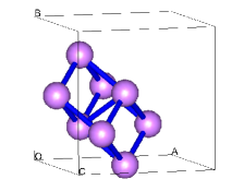
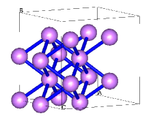
Figure 1: Bcc Li₈ (left panel) and Li₁₆ (right panel) clusters used to test PAW calculations.

Table 1: Equilibrium lattice constant for bcc-Li, $a$ (Bohr) and bulk modulus, $B$ (GPa).

		LDA				$\rm GGA$
Method	$r_{c}$	PW		PZ		PBE
		$a$	$B$	$a$	$B$	$a$	$B$
Abinit ($3e^{-}$, PAW, c.ch.)	1.61	6.363	15.1	–	–	6.513	14.0
Abinit ($3e^{-}$, PAW)	1.61	6.363	15.0	6.360	15.1	6.497	13.8
Abinit ($3e^{-}$, PAW)	0.80	6.362	15.1	6.359	15.1	6.497	13.9
Q-Espreso ($3e^{-}$, PAW, c.ch.)	1.61	6.364	15.0	–	–	6.516	14.1
Q-Espreso ($3e^{-}$, PAW, c.ch.)	0.80	6.362	15.0	–	–	6.497	13.8
Q-Espreso ($1e^{-}$)	–	–	–	6.320	15.1	6.724	11.9
Q-Espreso ($3e^{-}$)	–	–	–	6.362	15.1	6.500	13.8
Vasp ($1e^{-}$, PAW, c.ch.)	2.05	–	–	6.373	15.0	6.514	13.7
Vasp ($3e^{-}$, PAW, c.ch.)	1.55-2.00	–	–	6.362	14.9	6.505	13.8

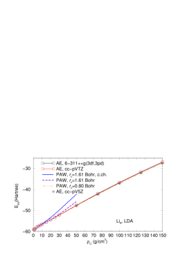
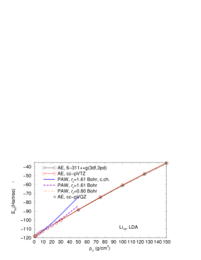
Figure 2: All-electron (VWN correlation) and PAW (PZ correlation) LDA total energies for the Li₈ and Li₁₆ clusters.

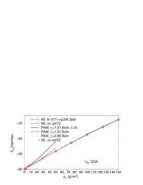
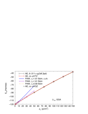
Figure 3: All-electron and PAW GGA total energies for the Li₈ and Li₁₆ clusters.

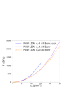
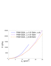
Figure 4: Pressure vs. material density from PAW LDA (PW correlation) (left panel) and from PAW GGA (PBE XC) (right panel) calculations for bulk bcc-Li.

The remaining validation issue is the effect of PAW or PP on the calculated pressure. A study Horner09 of the EOS for warm, dense LiH found that the $3e^{-}$ PAW for Li in VASP calculations was necessary for T = 2, 4, and 6 eV and densities twice that of ambient and greater. Fig. 4 shows the bulk bcc Li pressure as a function of material density at T=100 K calculated using Abinit with the same three PAW data sets as before for both the PW LDA and PBE XC functionals. (Use of the PZ LDA functional gives results indistinguishable from those from PW LDA on the scale of the figure.) One sees that the standard PAW data set (i) starts to overestimate the pressure at $\rho_{\rm Li}^{bulk-crit1}=6.0$ g/cm³ for LDA and at a slightly lower value for PBE. PAW data set (ii) produces results which agree with the reference calculations (i.e., those from PAW set (iii)) for densities up to $\rho_{\rm Li}^{bulk-crit2}=15.0$ g/cm³. Comparison of critical density values in the clusters and in bulk shows that $\rho_{\rm Li}^{bulk-crit1}$ is slightly lower than $\rho_{\rm Li}^{clust-crit1}$. A crude linear extrapolation of the results from PAW data sets (i) and (ii) gives an estimated lower bound for the critical bulk density for the reference PAW data set $\rho_{\rm Li}^{bulk-crit3}$ to be 80 g/cm³. Additional tests would be needed to get the actual value of $\rho_{\rm Li}^{bulk-crit3}$. Such a determination is not required for the present purposes.

We observe that for fcc Al at $\mathrm{T}$=0 K, Levashov et al.LevashovEtAl10 found that the standard VASP PAW pressures began to deviate materially from all-electron values at about a compression of seven. Since it was standard VASP, presumably that PAW included charge compensation, hence their result should correspond to our set (i) Li results, those labeled “PAW, $r_{c}$ = 1.61 bohr, c.ch.” in Fig. 4. It is clear that the deviation they found in fcc Al is at similar but modestly lower compression than we find for bcc Li.

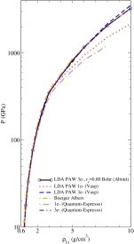
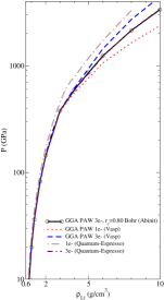
Figure 5: Validation of Vasp 1$e^{-}$, 3$e^{-}$ PAW, Quantum-Espresso 1$e^{-}$, 3$e^{-}$ PZ LDA (left panel) and Vasp 1$e^{-}$, 3$e^{-}$ PAW, Quantum-Espresso 1$e^{-}$, 3$e^{-}$ PBE GGA (right panel) pseudopotential calculations: pressure as a function of density for bcc-Li calculated at T=100 K.

Figure 5 compares pressure versus material density (T=100 K) for LDA (left panel) and PBE GGA (right panel) for material densities in the range $0.6-10.0$ g/cm³ obtained from Vasp and Quantum-Espresso using standard PPs (the PAW provided with the Vasp package and the norm-conserving PP taken from the Quantum-Espresso web page), and reference results obtained with our PAW data set (iii) (for both the PZ LDA and PBE GGA XC functionals.) For LDA, we also show the earlier all-electron results by Boettger and Albers Boettger.Albers.1989 . Observe first that our designation of the PAW (iii) as a reference is substantiated by the agreement with the all-electron LDA calculation. The Vasp $1e^{-}$ PAW LDA results start to deviate from the reference values at about 3.0 g/cm³. However the $3e^{-}$ PAW LDA pressure from Vasp is in good agreement for densities up to 6.0 g/cm³. Quantum-Espresso results calculated with the $1e^{-}$ PZ LDA pseudopotential start to deviate from the reference results for density between 2 and 3 g/cm³, whereas the $3e^{-}$ potential produces results which agree virtually perfectly for the full density range. For the GGA case, the right-hand panel of Fig. 5 shows that the situation is very similar except that both the $1e^{-}$ and $3e^{-}$ PAW Vasp calculations start to deviate from the reference results at almost the same density ($\approx 3$ g/cm³). Quantum-Espresso $1e^{-}$ calculations overestimate the pressure for $\rho_{\rm Li}>0.8$ g/cm³. However, the Quantum-Espresso $3e^{-}$ results are in virtually perfect agreement with the reference PAW results for the whole range of densities.

IV Finite temperatures

IV.1 Pseudopotentials and level populations

In finite-temperature calculations (either KS or HF), there is non-zero occupation of one-electron levels which correspond to empty levels at $\mathrm{T}=0$ K (virtual states or simply “virtuals”). Satisfaction of some computational threshold for the smallest non-negligible occupation number requires an increasingly large set of those virtuals to be considered with increasing $\mathrm{T}$. Concurrently there is depopulation of levels fully occupied at $\mathrm{T}=0$ K. One would hope that PP methods which treat all electrons self-consistently would be applicable for such finite-$\mathrm{T}$ calculations. A related issue is the validity of using PPs which remove some of the core. A rough estimate of the relevant scale comes from taking the $1s$ ionization potential for the Li atom to be approximately the magnitude of the LDA Kohn-Sham $1s$ eigenvalue, about 51 eV. Then PP treatment of Li $1s$ electrons as core might be expected to be applicable for temperatures much smaller than 51 eV. The question is the validity of any estimate of this sort, in particular, how much smaller? We remark that Levashov et al. LevashovEtAl10 found that for ambient density Al, the PAW pressure deviated from the all-electron value at about $\mathrm{T}$ = 5-6 eV. This is less than 10% of the magnitude of the LSDA 2p atomic KS eigenvalue (about 70 eV).

First consider the comparative performance of the PPs. Figure 6 shows the hydrostatic pressure as a function of temperature calculated using $1e^{-}$ and $3e^{-}$ norm-conserving pseudopotentials for the bcc-Li structure (fixed nuclear positions, $\rho_{\rm Li}=0.5$ and $1.0$ g/cm³). Notice that this calculation uses a ground-state XC functional: there is no explicit temperature dependence in the PZ LDA XC functional. If the number of bands taken into account for a two-atom unit cell for $\rho_{\rm Li}=0.5$ g/cm^-3 is 128, the occupation number of the highest energy bands is of the order of $10^{-6}-10^{-7}$. Observe that the results from the $1e^{-}$ PP are in almost perfect agreement with those from the $3e^{-}$ calculations for $\mathrm{T}$ up to 75,000 K, with small disagreement appearing at higher temperatures. For low to moderate compression, it appears that the range of applicability of standard $1e^{-}$ norm-conserving pseudopotentials is at least up to ${\mathrm{T}}=$ 100 kK or about 8 – 9 eV. This fits the rough argument based on the Li $1s$ KS eigenvalue, with the criterion for “much smaller” being of order 20 % at most.

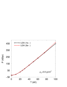
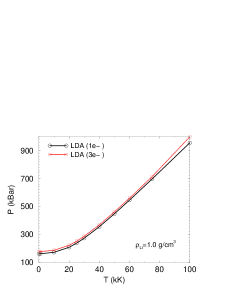
Figure 6: Comparison of pressure vs. temperature for bcc-Li obtained with 3${\it e-}$ and 1${\it e-}$ pseudopotentials for the Perdew-Zunger LDA exchange-correlation functional as implemented in Quantum-Espresso (2-atom unit cell, 9x9x9 k-mesh, 128 bands). Left panel: $\rho_{\rm Li}=0.5$ g/cm³. Right panel: $\rho_{\rm Li}=1.0$ g/cm³.

Next comes the matter of significant fractional occupation of ever-higher energy orbitals with increasing temperature. A related issue is energy level shifting and reordering with increased density, an effect known for ${\mathrm{T}}=0$K Li BoettgerTrickey85 ; ZittelEtAl85 .

Again, we did calculations with ground-state XC on bcc Li, with material density from 0.6 to 4.0 g/cm³. For all temperatures and densities, we used a 7 $\times$ 7 $\times$ 7 Monkhorst-Pack k-grid MonkhorstPack76 , a two-atom unit cell, and included 128 bands with a plane wave energy cutoff of 150 Ry. The calculations were done with Quantum-Espresso and the $1e^{-}$ PP just mentioned. The upper panel of Figure 7 shows a sample of the orbital eigenvalues for a single k-point, $\Gamma$, as a function of material density for ${\mathrm{T}}=100$ kK. The ${\mathrm{T}}=100$ K plot is absolutely indistinguishable, due to relatively small differences in the eigenvalues. The eigenvalues are labeled in order of increasing energy, $\varepsilon_{1}$ lowest, $\varepsilon_{128}$ highest. The main point to be noticed is that as the density increases, the spread in the lower half (roughly) of the eigenvalues increases. Those are the eigenvalues most pertinent to the calculation, in the sense that at a given temperature, excited levels will be depopulated at higher densities compared to the corresponding levels at lower densities. (An exception would be a pressure-induced switch in level-ordering.) The lower panels of Fig. 7 show the occupation numbers for those same eigenvalues. At low temperature and low density, the results are as expected, an almost square-wave Fermi distribution with the lowest band fully occupied (since there are two electrons in the unit cell) and the higher bands unoccupied. At higher densities, some k-points, including the $\Gamma$ point, as shown in the lower left panel, for densities above 3 g/cm³, have no occupation while others have two occupied levels. This repopulation is a consequence of changes in the KS orbitals caused by changes in the external potential, hence also in the effective KS potential. The lower right panel shows that at higher temperatures there is not only a temperature dependence of the occupation numbers, but a significant density dependence because of the spreading of the orbital energy levels.

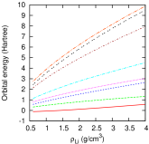
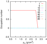
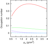
Figure 7: Top: orbital energies for the $\Gamma$ point, at 100 kK. Bottom left: single-spin occupation number $f_{i}$ of the levels plotted for $\mathrm{T}=100$ K. Bottom right: same but for $\mathrm{T}=100$ kK. The legend for the level number, given in the upper right, is for all plots.

Next we consider the number of bands required for a stipulated precision, given by a minimum occupation number threshold, as a function of temperature and density. For the calculations just discussed, we calculated a zone-averaged band occupation. For a band of composite index $i$, we sum the occupations of the $\varepsilon_{i}$ level multiplied by the k-point integration weight for all $\mathbf{k}$-points. This zone-averaged occupation is plotted for ${\mathrm{T}}=100$kK in Figure 8. One sees clearly that, for a given threshold in occupation number, for example $10^{-6}$, the number of required bands decreases significantly with increasing density. This decrease again is due to changes in the KS orbitals. At least at ${\mathrm{T}}=0$K, it long has been known BoettgerTrickey85 ; ZittelEtAl85 that as Li is compressed, its band structure initially becomes less like the homogeneous electron gas (HEG) than the bcc zero-pressure bands. However, eventually, the system passes over to a Thomas-Fermi-Dirac equation of state, signifying near-perfect but spread parabolic bands (see upper panel of Fig. 7) and corresponding HEG occupations.

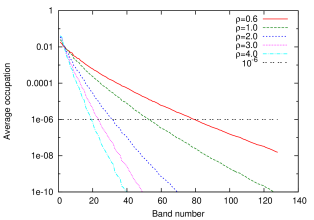
Figure 8: Zone-averaged band occupation numbers for all bands at $\mathrm{T}$ = 100 kK, for the various material densities listed.

IV.2 Exchange free energy

Though it originated in the Greens function formalism of many-fermion theory, the finite-temperature Hartree-Fock approximation is the thermodynamical generalization of the variational optimization of a single-determinant trial wave function which is ubiquitous in quantum-chemistry and molecular physics as the HF approximation Mermin63 .

To summarize, the thermal generalization of the familiar HF single-determinantal exchange energy may be expressed in terms of the one-electron reduced density matrix (1-RDM)

$${\mathcal{F}}_{\rm x}[n]:=-\int d{\mathbf{x}}_{1}\,d{\mathbf{x}}_{2}\,\{ g_{12}\bar{\Gamma}^{(1)}({\mathbf{x}}_{1}|{\mathbf{x}}_{2}^{\prime})$$

$$\times\bar{\Gamma}^{(1)}({\mathbf{x}}_{2}|{\mathbf{x}}_{1}^{\prime})\}_{{\mathbf{x}}_{1}^{\prime}={\mathbf{x}}_{1},{\mathbf{x}}_{2}^{\prime}={\mathbf{x}}_{2}}\,,$$ (7)

where ${\mathbf{x}}:={\mathbf{r}},s$ is a composite space-spin variable, $g_{12}=1/2{|{\mathbf{r}}_{1}-{\mathbf{r}}_{2}|}$, and the 1-RDM is defined in terms of the relevant orbitals $\{\varphi_{i}\}$ and occupation numbers $\{f_{i}\}$

$$\bar{\Gamma}^{(1)}({\mathbf{x}}_{1}|{\mathbf{x}}^{\prime}_{1}):=\sum_{j=1}^{\infty}f_{j}\varphi_{j}({\mathbf{x}}_{1})\varphi^{*}_{j}({\mathbf{x}}^{\prime}_{1})\,,$$ (8)

subject to

$$f_{j}\equiv f(\varepsilon_{j}-\mu)=[1+\exp(\beta(\varepsilon_{j}-\mu))]^{-1}$$ (9)

and

$$\int d{\mathbf{x}}\varphi_{i}({\mathbf{x}})\varphi^{*}_{j}({\mathbf{x}}) = \delta_{ij}$$

$$\sum_{j=1}^{\infty}f_{j} = N\;,$$ (10)

with $\beta:=1/k_{B}\rm T$ as usual. Here $\mu$ is the chemical potential (determined by Eq. (10)) and the $\varepsilon_{j}$ are the eigenvalues of the associated one-particle ftHF equation.

The analogue to ftHF in DFT is called finite-temperature exact exchange (ftEXX hereafter) DFT Greiner10 . In its pure Kohn-Sham form, ftEXX defines the exchange free energy formally identically with ftHF, but evaluates the density $n({\mathbf{r}},\rm T)$ from orbitals which follow from a true KS procedure, that is, from a one-body Hamiltonian with a local (multiplicative) exchange potential. That potential follows from the system response function, $\delta n/\delta v_{\rm KS}$. A full ftDFT calculation (not exchange only) would have a correlation free energy functional and associated KS potential as well.

Ground state DFT with so-called hybrid approximate exchange functionals has a similar structure for the total energy, in the sense that hybrids have contributions both from single-determinant exchange and from exchange-correlation functionals which are explicitly density dependent. Instead of a KS procedure, one can go from such a hybrid expression directly to coupled one-electron equations by explicit variation with respect to the orbitals. In ground-state theory with a hybrid functional, this procedure sometimes is called generalized KS. The relevant point is that the same approach applies directly to ftHF. Simply switch off the explicit density functionals for exchange and correlation and leave the exchange functional which comes from the trace over single-determinants. Since the capacity to do hybrid DFT as a generalized KS approach exists in both Vasp and Quantum-Espresso, one sees that such coding is immediately exploitable for doing ftHF.

In parallel with ground state DFT, an LDA may be obtained from considering the finite-$\mathrm{T}$ HEG. Its exchange free energy is given in first-order perturbation theory by

$${\mathcal{F}}_{\rm x}^{\rm HEG}=-\frac{V}{(2\pi)^{6}}\int\int d\mathbf{k}\;d\mathbf{k^{\prime}}\frac{4\pi}{\left|\mathbf{k}-\mathbf{k^{\prime}}\right|}f({\mathbf{k}})f({\mathbf{k^{\prime}}})$$ (11)

where $f(\mathbf{k})=[1+\exp(\beta(k^{2}/2-\mu^{\rm HEG}))]^{-1}$, and $V$ is the system volume. With the chemical potential expanded to the same order as well, $\mu^{\rm HEG}=\mu_{0}^{\rm HEG}+\mu_{\rm x}^{\rm HEG}$, the exchange portion is

$$\mu_{\rm x}^{\rm HEG}(n,{\rm T})=\frac{\delta{\mathcal{F}}_{\rm x}^{\rm HEG}}{\delta n}$$ (12)

If expressed in closed form, this result may be used as the finite-$\mathrm{T}$ LDA, with exchange free energy per electron $f_{\rm x}^{\rm LDA}(n(\mathbf{r},{\rm T}),{\rm T})=({\mathcal{F}}_{\rm x}^{\rm HEG}/nV)|_{n=n({\mathbf{r}},T)}$, and $v_{\rm x}^{\rm LDA}(n({\bf r},{\rm T}),{\rm T})=\mu_{\rm x}^{\rm HEG}(n,{\rm T})|_{n=n(\mathbf{r},{\rm T})}$. Here we used the parametrization given by Perrot and Dharma-wardana Perrot.Dharma-wardana.1984 . The LDA exchange free energy is then

$${\mathcal{F}}_{\rm x}^{\rm LDA}[n(\mathbf{r}),{\rm T}]=\int f_{\rm x}^{\rm LDA}(n(\mathbf{r},{\rm T}),{\rm T})n(\mathbf{r},{\rm T})d\mathbf{r}\,.$$ (13)

The one-particle density follows by obvious analogy with Eqs. 8 - 10.

IV.3 Finite-temperature Hartree-Fock and DFT X-only calculations

To study the importance of using an explicitly $\mathrm{T}$-dependent expression for the exchange free energy (rather than a calculation with a ground-state X functional) and to estimate the quality of the $\mathrm{T}$-dependent exchange free-energy functional defined by Eq. (13), we compare ftHF calculations which use the exact exchange free energy Eq. (7), Kohn-Sham calculations with $\mathrm{T}$-independent LDA exchange for the exchange free energy, ${\mathcal{F}}_{\rm x}\approx E_{\rm x}^{\rm LDA}$, and KS calculations done with the $\mathrm{T}$-dependent exchange free energy functional ${\mathcal{F}}_{\rm x}^{\rm LDA}$. In the following discussion, the ground-state functional calculations are labeled “LDAx”, while those which used the explicitly $\mathrm{T}$-dependent LDA are labeled “LDAx(T)”. All the calculations were done with Quantum-Espresso using the $1e^{-}$ PZ LDA pseudopotential taken from the Quantum-Espresso web page. We treated bcc Li with fixed nuclear positions, here with densities between $\rho_{\rm Li}=0.6$ and $1.8$ g/cm³ and temperatures between 100K and 100kK. At these densities and temperatures, the Quantum-Espresso $1e^{-}$ pseudopotential is adequate; recall Sections III.2 and IV.1 as well as Figs. 5 and 6.

Convergence of the ftHF and the LDAx calculations with respect to the ${\mathbf{k}}$-mesh for the bcc-Li 2-atom unit cell requires attention. It is known DacorognaCohen86 that T=0 K LDA calculations on bcc Li exhibit misleading convergence behavior at a relatively coarse $\mathbf{k}$-mesh density. We tested for the smallest real space cell size used, corresponding to bulk density $\rho_{\rm Li}=1.8$ g/cm³. The ftHF total free energy calculations converge much more slowly than the ftDFT calculations. For the moderate $7\times 7\times 7$ ${\mathbf{k}}$-mesh, the DFT calculations are converged to an iteration-to-iteration difference of 0.02 eV per atom, while the HF calculations converge to the same precision only upon reaching the much denser $17\times 17\times 17$ mesh. Moreover, the HF calculation exhibits a potentially misleading energy minimum at $15\times 15\times 15$. The ${\mathbf{k}}$-mesh convergence becomes faster with increasing $\mathrm{T}$. For example, at $\mathrm{T}$ = 100 kK, both HF and LDAx calculations already are converged at the $3\times 3\times 3$ ${\mathbf{k}}$-mesh. In all calculations, both HF and DFT, presented in this section, the $25\times 25\times 25$ ${\mathbf{k}}$-mesh was used.

Figure 9 compares changes in the exchange free energy contribution with increasing $\mathrm{T}$ relative to 100K values, ${\mathcal{F}}_{\rm x}({\rm T})-{\mathcal{F}}_{\rm x}(\rm 100K)$. The $\mathrm{T}$-independent LDA exchange free energy practically does not change over that range, i.e., ${\mathcal{F}}_{\rm x}^{\rm LDA}[n({\bf r},{\rm T})]\approx{\mathcal{F}}_{\rm x}^{\rm LDA}[n({\bf r},\rm 100K)]$. In contrast, the HF exchange free energy increases significantly (by about 4-5 eV per atom) with increasing $\mathrm{T}$. The $\mathrm{T}$-dependent LDA exchange free energy reproduces the HF behavior at least qualitatively.

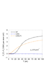
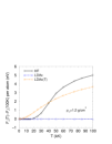
Figure 9: Comparison of finite-temperature HF, ground state LDA X-only (LDAx) and $\mathrm{T}$-dependent LDA X-only (LDAx(T)) exchange free energy differences $\Delta{\mathcal{F}}_{\rm x}({\rm T})={\mathcal{F}}_{\rm x}({\rm T})-{\mathcal{F}}_{\rm x}(100{\rm K})$ per atom as a function of electronic temperature $\mathrm{T}$. Left panel: $\rho_{\rm Li}=0.6$ g/cm³; right panel: $\rho_{\rm Li}=1.2$ g/cm³.

The exchange free energy is, of course, a small portion of the total free energy. Figure 10 shows total free energy differences $\Delta{\mathcal{F}}_{\rm tot}({\rm T})={\mathcal{F}}_{\rm tot}({\rm T})-{\mathcal{F}}_{\rm tot}(100{\rm K})$ as a function of electronic temperature. The free energy is monotonically decreasing with increasing $\mathrm{T}$, in agreement with non-negativity of the entropy evaluated from the thermodynamic relation ${\mathcal{S}}=-\frac{\partial{\mathcal{F}}}{\partial\rm T}\Big{|}_{N,V}$. The DFT X-only total free energies from $\mathrm{T}$-independent LDA X lie below the corresponding ftHF values for all $\mathrm{T}$ and both densities. At $\mathrm{T}\approx 20$ kK, the interval is about 2 eV/atom, growing to about 4-5 eV/atom by 40 kK. The $\mathrm{T}$-dependent LDA X gives total free energy behavior much closer to that of ftHF, with discrepancies not exceeding $1-2$ eV/atom.

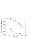
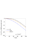
Figure 10: Comparison of finite-temperature HF, ground state LDA X-only (LDAx) and $\mathrm{T}$-dependent LDA X-only (LDAx(T)) total free energy differences $\Delta{\mathcal{F}}_{\rm tot}({\rm T})={\mathcal{F}}_{\rm tot}({\rm T})-{\mathcal{F}}_{\rm tot}(100{\rm K})$ per atom as a function of electronic temperature. Left panel: $\rho_{\rm Li}=0.6$ g/cm³; right panel: $\rho_{\rm Li}=1.2$ g/cm³.

The effect of explicit $\mathrm{T}$-dependence in exchange upon the pressure may be estimated from the difference between the ftHF or LDAx(T) and the LDAx values. Figure 11 provides this comparison. As a function of $\mathrm{T}$, the pressure from ftHF starts below the LDAx curve, then crosses and goes above it at about 55-75 kK, depending upon the material density. The temperature of this crossing point increases slightly with material density. To isolate the effect of exact $\mathrm{T}$-dependent X upon the pressure, we consider the difference between ftHF and LDAx values, offset by the near-zero-temperature difference

$$\Delta P_{\rm HF-LDAx}({\rm T})=P_{\rm HF}({\rm T})-P_{\rm LDAx}({\rm T})$$ (14)

at ${\mathrm{T}}=$ 100K, i.e.,

$$\Delta\Delta P_{\rm HF-LDAx}({\rm T}) = \Delta P_{\rm HF-LDAx}({\rm T})$$ (15)

$$-\Delta P_{\rm HF-LDAx}({\rm 100K})\;.$$

One can see from the right-hand panels of Fig. 11 that the maximum magnitude of this difference at $\mathrm{T}$= 100 kK is about 10 % for all material densities considered. For low temperatures, the effect of exact $\mathrm{T}$-dependent X on pressure is stronger. For example, at 30 kK $\Delta\Delta P_{\rm HF-LDAx}({\rm 30kK})\approx 5$ GPa for material density 1.0 g/cm³, the shift is $\approx$ 30% of the HF pressure (about 15 GPa) at that $\mathrm{T}$. Again, the LDAx(T) and ftHF temperature-dependence resemble one another qualitatively whereas the LDAx result does not. Note that the LDAx(T) crossing temperature with respect to the LDAx curve increases much more rapidly with increasing material density than for ftHF. For material density $\rho_{\rm Li}=0.6$ g/cm³, both curves cross at ${\mathrm{T}}\approx 60$ kK. At $\rho_{\rm Li}=1.2$ g/cm³ the LDAx(T) pressures crosses the LDAx curve at ${\mathrm{T}}\approx$ 100 kK, higher than the temperature of the HF-LDAx crossing point ${\mathrm{T}}\approx$ 70 kK. With increasing material density the shift between LDAx(T) and ftHF increases especially for ${\mathrm{T}}\geq$ 50 kK.

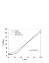
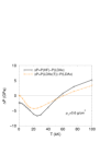
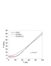
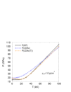
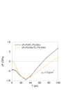
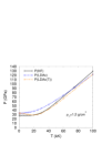
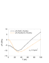
Figure 11: Effect of temperature-dependent exchange on pressure. Left panels: pressure as a function of electronic temperature as predicted by HF, LDAx, and LDAx(T) calculations for $\rho_{\rm Li}=0.6,0.8,1.0$ and $1.2$ g/cm³. Right panels: differences in pressure between calculations with $\mathrm{T}$-dependent and $\mathrm{T}$-independent X, $\rm P(HF)-P(LDAx)$ and $\rm P(LDAx(T))-P(LDAx)$.

V Conclusions

Detailed computational examination of the applicability of standard PP and PAW methods to the WDM regime, with bulk Li as the test system, yields several insights. By unambiguous comparison with all-electron results from small Li clusters of bcc-derived symmetry, we find that the PAW scheme requires a small augmentation sphere radius, that the compensation-charge term is not helpful, and that all electrons must be treated in the SCF calculation. We have constructed such PAW data sets for LDA and GGA functionals and used them to generate reference data.

We have located the maximal material density of bulk bcc-Li usable for standard PPs in Vasp, Abinit, and Quantum-Espresso codes. And we have delineated the validity of using such PPs at high $\mathrm{T}$ by comparison of $1e^{-}$ and $3e^{-}$ PP results. The transferability of PPs and PAW data sets developed for near-equilibrium conditions to the WDM regime is conditional. At near-equilibrium densities it appears to be acceptable, but not at high densities. Clearly, such transferability should not be assumed.

With these issues settled, we have found that there is non-trivial effect of explicit $\mathrm{T}$-dependence in the X functional in the specific sense of comparison with ftHF. In particular, the LDA $\mathrm{T}$-dependent exchange contribution to the total free energy is much closer to the exact HF exchange value than is the contribution from exchange approximated by the LDA ground-state X functional. Although the exchange free energy is a small portion of the total free energy, this difference carries over into clearly significant differences in the equation of state. Thus, the effect of explicit $\mathrm{T}$-dependence in X is relevant for an accurate characterization of the Li equation of state in the WDM regime. We suspect that this may be generally true of WDM systems. If so, $\mathrm{T}$-dependent LDA exchange may serve as a starting point for development of more refined GGA-type exchange free energy functionals, analogous with the role of LDA in the ground state.

VI Acknowledgments

We acknowledge, with thanks, many informative conversations with our colleagues J.W. Dufty, F.E. Harris, and K. Runge. SBT also thanks M. Desjarlais, F. Lambert, and L. Collins for informative discussions. Work supported in part under U.S. Dept. of Energy BES (TCMP, TMS) grant DE-SC 0002139.

References

- (1) Report of the Workshop on High Energy Density Laboratory Physics Research Needs. The U.S. Department of Energy, Office of Science and National Nuclear Security Administration (2009).
- (2) N.D. Mermin, Phys. Rev. 137, A1441 (1965).
- (3) M.V. Stoitsov and I.Zh. Petkov, Annals Phys. 185, 121 (1988).
- (4) R.M. Dreizler in The Nuclear Equation of State, Part A, W. Greiner and H. Stöcker eds., NATO ASI B216 (Plenum, NY, 1989) 521.
- (5) A. Alavi, J. Kohanoff, M. Parrinello, and D. Frenkel, Phys. Rev. Lett. 73, 2599 (1994).
- (6) P.L. Silvestrelli, Phys. Rev. B 60, 16382 (1999) and refs. therein.
- (7) M.P. Surh, T.W. Barbee III, and L.H. Yang, Phys. Rev. Lett. 86, 5958 (2001).
- (8) M.P. Desjarlais, J.D. Kress, and L.A. Collins, Phys. Rev. E 66, 025401 (2002).
- (9) S.A. Bonev, B. Militzer, and G. Galli, Phys. Rev. B 69, 014101 (2004).
- (10) S. Mazevet, P. Blottiau, J.D. Kress, and L.A. Collins, Phys. Rev. B 69, 224207 (2004).
- (11) L.A. Collins, J.D. Kress, and S.F. Mazevet, Los Alamos Science, Number 29, 70–79 (2005) and references therein.// http://library.lanl.gov/cgi-bin/getfile?29-06.pdf
- (12) S. Mazevet, M.P. Desjarlais, L.A. Collins, J.D. Kress, and N.H. Magee, Phys. Rev. E 71, 016409 (2005).
- (13) V. Recoules, J. Clérouin, G. Zérah, P.M. Anglade, and S. Mazevet, Phys. Rev. Lett. 96, 055503 (2006).
- (14) G. Faussurier, P.L. Silvestrelli, and C. Blancard, High En. Dens. Phys. 5, 74 (2009).
- (15) D.A. Horner, F. Lambert, J.D. Kress, and L.A. Collins, Phys. Rev. B 80, 024305 (2009).
- (16) V. Recoules, F. Lambert, A. Decoster, B. Canaud, and J. Clérouin, Phys. Rev. Lett. 102, 075002 (2009).
- (17) S.M. Vinko, G. Gregori, M.P. Desjarlais, B. Nagler, T.J. Whitcher, R.W. Lee, P. Audebert, and J.S. Wark, High En. Dens. Phys. 5, 124 (2009).
- (18) K. Wünsch, J. Vorberger, and D.O. Gericke, Phys. Rev. E 79, 010201(R) (2009).
- (19) J. Clérouin, C. Starrett, G. Faussurier, C. Blancard, P. Noiret, and P. Renaudin, Phys. Rev. E 82, 046402 (2010).
- (20) G. Kresse and J. Hafner, Phys. Rev. B, 47, 558 (1993), ibid. 49, 14251 (1994); G. Kresse and J. Furthmüller, Comput. Mat. Sci. 6. 15 (1996); Phys. Rev. B, 54, 11169 (1996).
- (21) X. Gonze, B. Amadon, P.-M. Anglade, J.-M. Beuken, F. Bottin, P. Boulanger, F. Bruneval, D. Caliste, R. Caracas, M. Cote, T. Deutsch, L. Genovese, Ph. Ghosez, M. Giantomassi, S. Goedecker, D.R. Hamann, P. Hermet, F. Jollet, G. Jomard, S. Leroux, M. Mancini, S. Mazevet, M.J.T. Oliveira, G. Onida, Y. Pouillon, T. Rangel, G.-M. Rignanese, D. Sangalli, R. Shaltaf, M. Torrent, M.J. Verstraete, G. Zerah, and J.W. Zwanziger, Comput. Phys. Commun. 180, 2582 (2009); X. Gonze, G.-M. Rignanese, M. Verstraete, J.-M. Beuken, Y. Pouillon, R. Caracas, F. Jollet, M. Torrent, G. Zerah, M. Mikami, Ph. Ghosez, M. Veithen, J.-Y. Raty, V. Olevano, F. Bruneval, L. Reining, R. Godby, G. Onida, D.R. Hamann, and D.C. Allan, Zeit. Kristallogr. 220, 558 (2005).
- (22) S.H. Vosko, L. Wilk, and M. Nusair, Can. J. Phys. 58, 1200 (1980).
- (23) J.P. Perdew, and A. Zunger, Phys. Rev. B 23, 5048 (1981).
- (24) J.P. Perdew, and Y. Wang, Phys. Rev. B 45, 13244 (1992).
- (25) J.P. Perdew, K. Burke, and M. Ernzerhof, Phys. Rev. Lett. 77, 3865 (1996); erratum ibid. 78, 1396 (1997).
- (26) J.-F. Danel, L. Kazandjian, and G. Zérah, Phys. Plasmas 13, 092701 (2006).
- (27) S. Tanaka, S. Mitake, and S. Ichimaru, Phys. Rev. A 32, 1896 (1985).
- (28) K. Burke, J.P. Perdew, and Y. Wang, in Electronic Density Functional Theory: Recent Progress and New Directions, J.F. Dobson, G. Vignale, and M.P. Das eds (Plenum Press NY, 1998) 81-111.
- (29) F. Perrot and M.W.C. Dharma-wardana, Phys. Rev. B 62, 16536 (2000); ibid. 67, 079901(E) (2003).
- (30) R.P. Feynman, N. Metropolis, and E. Teller, Phys. Rev. 75, 1561 (1949).
- (31) D.A. Liberman, Phys. Rev. B 20, 4981 (1979).
- (32) B.F. Rozsnyai, Phys. Rev. A 5 1137, (1972); ibid. 43, 3035 (1991).
- (33) B. Wilson, V. Sonnad, P. Sterne, and W. Isaacs, J. Quant. Spectrosc. Radiat. Transfer 99, 658 (2006).
- (34) C.E. Starrett and D. Saumon, High En. Dens. Phys. 8, 101 (2012).
- (35) S. Mazevet, F. Lambert, F. Bottin, G. Zérah, and J. Clérouin, Phys. Rev. E 75, 056404 (2007).
- (36) P.R. Levashov, G.V. Sińko, N.A. Smirnov, D.V. Minakov, O.P. Shemyakin, and K.V. Kihishchenko, J. Phys. Condens. Matt. 22, 505501 (2010).
- (37) N.A.W. Holzwarth, A.R. Tackett, and G.E. Matthews, Comput. Phys. Commun. 135, 329 (2001).
- (38) Paolo Giannozzi, Stefano Baroni, Nicola Bonini, Matteo Calandra, Roberto Car, Carlo Cavazzoni, Davide Ceresoli, Guido L. Chiarotti, Matteo Cococcioni, Ismaila Dabo, Andrea Dal Corso, Stefano de Gironcoli, Stefano Fabris, Guido Fratesi, Ralph Gebauer, Uwe Gerstmann, Christos Gougoussis, Anton Kokalj, Michele Lazzeri, Layla Martin-Samos, Nicola Marzari, Francesco Mauri, Riccardo Mazzarello, Stefano Paolini, Alfredo Pasquarello, Lorenzo Paulatto, Carlo Sbraccia, Sandro Scandolo, Gabriele Sclauzero, Ari P. Seitsonen, Alexander Smogunov, Paolo Umari, and Renata M. Wentzcovitch, J. Phys.: Condens. Matter 21, 395502 (2009).
- (39) Gaussian 03, Revision C.02, M.J. Frisch, G.W. Trucks, H.B. Schlegel, G.E. Scuseria, M.A. Robb, J.R. Cheeseman, J.A. Montgomery, Jr., T. Vreven, K.N. Kudin, J.C. Burant, J.M. Millam, S.S. Iyengar, J. Tomasi, V. Barone, B. Mennucci, M. Cossi, G. Scalmani, N. Rega, G.A. Petersson, H. Nakatsuji, M. Hada, M. Ehara, K. Toyota, R. Fukuda, J. Hasegawa, M. Ishida, T. Nakajima, Y. Honda, O. Kitao, H. Nakai, M. Klene, X. Li, J.E. Knox, H.P. Hratchian, J.B. Cross, V. Bakken, C. Adamo, J. Jaramillo, R. Gomperts, R.E. Stratmann, O. Yazyev, A.J. Austin, R. Cammi, C. Pomelli, J.W. Ochterski, P.Y. Ayala, K. Morokuma, G.A. Voth, P. Salvador, J.J. Dannenberg, V.G. Zakrzewski, S. Dapprich, A.D. Daniels, M.C. Strain, O. Farkas, D.K. Malick, A.D. Rabuck, K. Raghavachari, J. B. Foresman, J.V. Ortiz, Q. Cui, A.G. Baboul, S. Clifford, J. Cioslowski, B.B. Stefanov, G. Liu, A. Liashenko, P. Piskorz, I. Komaromi, R.L. Martin, D.J. Fox, T. Keith, M.A. Al-Laham, C.Y. Peng, A. Nanayakkara, M. Challacombe, P.M.W. Gill, B. Johnson, W. Chen, M.W. Wong, C. Gonzalez, and J.A. Pople, Gaussian, Inc., Wallingford CT, 2004.
- (40) M. Torrent, N.A.W. Holzwarth, F. Jollet, D. Harris, N. Lepley, and X. Xu, Comput. Phys. Commun. 181, 1862 (2010).
- (41) M. Torrent, F. Jollet, F. Bottin, G. Zérah, and X. Gonze, Comput. Mater. Sci. 42, 337 (2008).
- (42) P. E. Blöchl, Phys. Rev. B 50, 17953 (1994).
- (43) G. Kresse, and D. Joubert, Phys. Rev. B 59, 1758 (1999).
- (44) J.C. Boettger and S.B. Trickey, Phys. Rev. B 32, 3391 (1985).
- (45) http://www.wfu.edu/ natalie/papers/pwpaw/periodictable/atoms/Li/index.html
- (46) J.P. Perdew, K. Burke, and M. Ernzerhof, Phys. Rev. Lett. 77, 3865 (1996); erratum ibid. 78, 1396 (1997).
- (47) A.B. Alchagirov, J.P. Perdew, J.C. Boettger, R.C. Albers, and C. Fiolhais, Phys. Rev. B 63, 224115 (2001).
- (48) J.C. Boettger, and R.C. Albers, Phys. Rev. B 39, 3010 (1989).
- (49) W.G. Zittel , J. Meyer-ter-Vehn, J.C. Boettger, and S.B. Trickey, J. Phys. F: Met. Phys. 15, L247 (1985).
- (50) H.J. Monkhorst and J.D. Pack, Phys. Rev. B 13, 5188 (1976).
- (51) N.D. Mermin, Annals Phys. 21, 99 (1963).
- (52) M. Greiner, P. Carrier, and A. Görling, Phys. Rev. B 81, 155119 (2010).
- (53) F. Perrot and M.W.C. Dharma-wardana, Phys. Rev. A, 30 2619 (1984).
- (54) M.M. Dacorogna and M.L. Cohen, Phys. Rev. B 34, 4996 (1986).