Batch Spreadsheet for C Programmers

Abstract

A computing environment is proposed, based on batch spreadsheet processing, which produces a spreadsheet display from plain text input files of commands, similar to the way documents are created using LaTeX. In this environment, besides the usual spreadsheet rows and columns of cells, variables can be defined and are stored in a separate symbol table. Cell and symbol formulas may contain cycles, and cycles which converge can be used to implement iterative algorithms. Formulas are specified using the syntax of the C programming language, and all of C’s numeric operators are supported, with operators such as ++, +=, etc. being implicitly cyclic. User–defined functions can be written in C and are accessed using a dynamic link library. The environment can be combined with a GUI front-end processor to enable easier interaction and graphics including plotting.

Keywords: Computational models, Software architectures for scientific computing

1 Introduction

The idea for a batch spreadsheet processor was originally proposed in [1] in the context of a course on parser design. The evolution of that idea presented here, which goes far beyond what was originally envisioned and implemented in the course, is based on the premise of enabling anything that seems reasonable, even if the usefulness is not immediately apparent. So, for example, if formula syntax is based on the C programming language, then it should support all of C’s operators, including ++, +=, etc. This is discussed further in Section 13 on cycles. Other examples, where the usefulness is apparent and the behavior intuitively expected, are allowing lists (such as function arguments) to be specified using cell ranges, cell ranges to be specified using single cells (for a single–cell range), and ranges to overlap and be specified in reverse and by columns or rows as discussed in Section 5.

After a brief review of the history of spreadsheets, we will present the specifications for the proposed batch processor, together with some examples from a partial implementation.

2 Spreadsheet History

The history of electronic spreadsheets [2] starts with Richard Mattessich [3] in 1964. The output of his batch processor looked like a spreadsheet, but the input was purely data and all functionality was encoded in the FORTRAN program implementing the business budget model. In all subsequent spreadsheet implementations, including the one proposed here, the input specifies both the data and the functional relationships among the cells.

The modern interactive spreadsheet era starts in 1979 with Visicalc, by Dan Bricklin and Bob Frankston. In 1982 James Gosling created the Unix SC spreadsheet calculator which has evolved through the work of others and is still in use today. In 1983 came Lotus 1-2-3, by Mitch Kapor, and in 1985 Excel for Macintosh, by Microsoft (Windows came later). There was also Quattro Pro, by Borland, in 1987, but in the battle for the commercial spreadsheet market eventually Excel won. Other popular opensource spreadsheet implementations include Oleo (1992) and Gnumeric, from the GNU Project, 1998, and OpenOffice, from StarOffice and Sun, 2000.

It is well-known that spreadsheet design and use can be very error-prone [4, 5], and most of the problems stem from the interactive nature of modern spreadsheet features such as cut/paste, adding and removing rows and columns, etc. The batch approach eliminates many of the traditional problems, while enabling more powerful command-line types of options. For example, to copy the entries from one range of cells to another, a copy command like copy a2:c6 d6:b2 allows overlapping and reverse ranges. A batch spreadsheet processor can also be written using portable C code, with no system-dependent GUI. For ease of discussion, we will refer to the batch spreadsheet for C programmers as simply “SS” for the rest of the paper.

3 Input and Output

SS first reads input from any files specified on the command line, then it reads standard input for additional commands such as may be supplied by a front-end GUI, or by the user directly. The input may contain C or C++ style comments, and macros using #define. As in C, input lines are joined together whenever one ends with a backslash followed by a literal newline character.

Output goes to standard output by default, but can be redirected globally using the output command, or redirected on a per–command basis using the plot and print commands. “stdout” and “-”, with or without quotes, can be used as pseudo output file names to refer to standard output.

4 Cell References

Cell references may be specified in any one of three formats: A0, RC, and CR. In A0 format, cells are specified by their column (one or two letters, A-Z, case-insensitive) and row (one-to-three digits 0-9), with an optional $ preceding the column and/or row value to indicate that the cell is fixed. The column value A…ZZ represents an integer column number 0…701. In RC and CR formats, cell are specified by their absolute row and column numbers, using the letters R and C (or r, c), with brackets around relative offsets.

When copying formulas, relative cell references remain relative to the destination cells, and fixed references remain fixed. The format for displaying cells in formulas may be selected using the format command.

5 Ranges

A range consists of two cells, the start and end cells of the range, separated by a colon. For example, A0:B9 (or A0:C1R9, or R0C0:R9C1, or C0R0:R9C1, etc.) specifies a range including rows 0 to 9 of columns A and B. The range start and end values do not have to be in increasing order; B9:A0, B0:A9, and A9:B0 all refer to the same group of cells as A0:B9, but correspond to different directions for traversing the range. For example the command copy a0:a9 b9:b0 would copy column b to a in reverse order.

By default, ranges are traversed byrows to improve cache performance, since elements in a row are adjacent in memory. That is, in pseudo-code:

  for row = start_row to end_row
    for col = start_col to end_col
      use cell[row,col]

The bycols option can be used with the copy, eval, fill, plot, and print commands to cause evaluation by columns. That is, in pseudo-code:

  for col = start_col to end_col
    for row = start_row to end_row
      use cell[row,col]

Note that the starting row may be less than, equal to, or greater than the ending row. Same for columns. So a range may consist of a single cell, row, or column (a0:a0, a0:d0, a0:a4), cells in “forward” order (a0:b4), or cells in “partial reverse” order (a4:b0, b0:a4), or cells in “reverse” order (b4:a0).

A range basically represents a list of cells, and is explicitly converted to a list when used in a range assignment or numeric function argument. A range consisting of a single cell may be specified using just that one cell, e.g. A0 as a range is the same as A0:A0.

6 Primitive Data Types

The SS primitive data types are double precision floating point, string, and constant. All numeric calculations are performed and stored using double precision floating point. A string is a sequence of characters enclosed in single or double quotes. No escape sequences are recognized. If a string appears in a numeric calculation it is treated as having the value 0. The built-in constants are: HUGE_VAL = Inf; RAND_MAX = 32767; pi = 3.14159 (computed from 4*atan(1)). The values of the constants shown are from a Solaris/sparc system and may vary depending on the system. Undefined cells are treated as having the value 0.

7 Symbols

User-defined variables are stored in a symbol table and their formulas are evaluated each time the spreadsheet is evaluated. Note that cell names can not be used as variables. See Sections 12 and 13 for examples using symbols.

8 Operators

SS operators have the same precedence and associativity as those in the C programming language. They mostly have the same meaning too, except for some of the bitwise operators. The keywords NOT, AND, XOR, and OR, case–insensitive, may also be used to represent the logical operators. The bit shift operators <<, <<=, >>, and >>= are implemented for floating-point using ldexp() to adjust the binary exponent by the specified power of 2. Additionally, C’s bitwise operators are treated as logical operators, so ~, &, ^, | are the same as !, &&, ^^ (logical XOR), || respectively, and &=, ^=, |= are the same as &&=, ^^=, ||=.

9 Numeric Functions

SS includes all of the functions from the standard C math library, and more. It includes the time function from time.h, rand and srand from stdlib.h, and also irand, drand, and nrand functions for integer, uniform(0,1), and normally distributed pseudo–random values respectively.

Most of the numeric functions take one expression argument and return one value. A few of the functions take no arguments (rand, irand, drand, nrand, time), and some take two arguments (atan2, fmod, frexp, ldexp, modf, pow). For frexp and modf, the second argument must be a cell or symbol, since it will be assigned one of the result values.

10 Range Functions

Range functions take an argument list of expressions and ranges and return one value computed from the defined cells. The range functions include:

  avg       average
  count     number of cells defined
  majority  non-zero if majority are non-zero
  max       maximum
  min       minimum
  prod      product
  stdev     standard deviation
  sum       sum

User–defined numeric and range functions can be written in C following a provided template to access SS internal data structures. These are loaded at run–time from a dynamic link library.

11 Commands

Commands have their own syntax, consisting of keywords and options. For all commands which traverse a range the byrows or bycols option may be used to set the direction. SS commands include:

  byrows|bycols - set default direction
  copy dest_range src_range
  debug [on|off]
  eval [range|symbols] [number_of_iterations]
  exit
  fill range start_expr, increment_expr
  format A0|RC|CR - formula printing format
  format [cell|row|col|range] "fmt_string"
  load "fname"...
  output "fname"
  plot|plot2d|plot3d ["fname"] [range]
  print ["fname"] [range] [all|
    macros|symbols|formulas|values|
    formats|pointers|constants|functions]...
  quit
  srand expr - initialize rand()

If no range or symbols options are specified, eval evaluates the spreadsheet for the number of iterations specified (default is 2 iterations). Each iteration first evaluates the symbol table, then evaluates the cells twice: first starting at the top-left corner of the cells being used and traversing the range to the bottom-right corner of the cells being used; then again starting at the bottom-right corner and traversing to the top-left corner. This catches most forward and reverse formula dependencies. If the symbols option is specified, only the symbol table is evaluated for the number of iterations specified. If a range is specified, only the symbol table and that range are evaluated for the number of iterations specified.

The fill command fills a range with constant values, starting with the start expression value, and increasing by the increment expression value for subsequent cells. The start and increment expressions are evaluated only once, before filling starts.

The format A0, RC, and CR options specify the format used for printing formulas. For printing values, the format can be set globally or for a specific cell, row, column or range. The default global format is “%.2f”. If a cell is not assigned a format, printing will use the cell’s row format, if set; otherwise it will use the cell’s column format, if set; otherwise it will use the global format.

The plot commands do not actually plot anything, they simply display output in a form suitable as input to another program like a plot utility.

12 Example

The following example shows a set of student scores being scaled by their average and standard deviation. Columns A and B represent the “natural” use of a spreadsheet for lists of values related to or computed from a parallel list of values. Cells C1 and D1 represent an “unnatural” situation which can occur frequently in spreadsheets where we need to store values somewhere, but their exact position does not matter relative to anything else. It would be more natural to store these types of values in variables instead of a spreadsheet cell. The example does that for the computation of the mean, in variable mean, and the use of that variable in the formula for column A is more “natural” and readable than the use of $d$1 for the standard deviation.

% cat grades.ss
a0:d0 = { "grade", "score", "avg", "stdev"};
mean=avg(b1:b5); c1=mean; d1=stdev(b1:b5);
a1=80+15*(b1-mean)/$d$1; copy a2:a5 a1:a4;
b1:b5 = { 57, 67, 92, 87, 76 }; eval;
print symbols values formulas pointers;
% ss < grades.ss

mean = avg(B1:B5) = 75.8    (symbols)

        A       B       C       D
0       grade   score   avg     stdev
1       60.29   57.00   75.80   14.31
2       70.77   67.00
3       96.98   92.00       (values)
4       91.74   87.00
5       80.21   76.00

        A
0       "grade"
1       80+((15*(B1-mean))/$D$1)
2       80+((15*(B2-mean))/$D$1)
3       80+((15*(B3-mean))/$D$1)
4       80+((15*(B4-mean))/$D$1)
5       80+((15*(B5-mean))/$D$1)

        B       C       D
0       "score" "avg"   "stdev"
1       57      mean    stdev(B1:B5)
2       67
3       92                  (formulas)
4       87
5       76

        A       B       C       D
0       1058e28 1058e60 1058e98 1058ed0
1       1059288 0       1058fb0 1059058
2       1059288 0
3       1059288 0           (pointers)
4       1059288 0
5       1059288 0

From the “print pointers” output at the end we can see that cells A1:A5 all refer to the same formula.

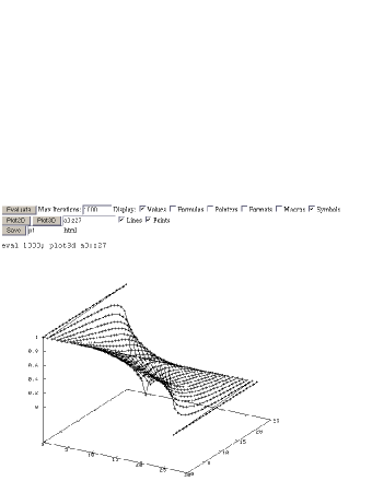
Figure 1: Spreadsheet GUI with 3D Plot

13 Cycles and Convergence

If a cell depends on itself, that forms a cycle and the spreadsheet may not converge when evaluated. Cycles which converge can be used to implement iterative algorithms. For example, the following spreadsheet uses Newton’s method to find the square root of x:

% cat sqrt.ss
x = 2; a0 = b0 ? b0 : x/2; b0 = (a0+x/a0)/2;
format "%20.18g";

Since a0 depends on b0, and b0 depends on a0, there is a cycle. a0 will be set to b0 if b0 is non-zero, otherwise a0 will be set to x/2 to initialize the algorithm. So a0 represents the previous value of b0, and b0 represents the next estimate of the square root. Newton’s method converges quickly:

% echo "print all; eval a0:b0 10; \
print values;" | ss sqrt.ss

x = 2

  A                    B
0 B0 ? B0 : ((x/2))    (A0+(x/A0))/2

  A                    B
0 0                    0

ss_eval:: converged after 7 iterations

  A                    B
0 1.41421356237309492  1.41421356237309492

Finite element analysis is another application which requires iteration and can be set up in a spreadsheet. In the following small example, the value of each non-boundary cell is computed as the average of the cell’s four nearest neighbors.

% cat cycles.ss
// average of 4 nearest neighbors
R1C1=(R[]C[-1]+R[]C[+1]+R[-1]C[]+R[+1]C[])/4;
copy r1c2:r1c5 r1c1:r1c4;// set up one row
copy r2c1:r5c5 r1c1:r4c5;// copy to rows 2..5
fill r0c0:r0c6 1, 0;// boundary conditions,
fill r1c0:r6c0 1, 0;//  1’s top and left
fill r1c6:r6c6 0, 0;//  0’s right and bottom
fill r6c1:r6c5 0, 0;
format "%6.4f"; format RC; print values;
eval; eval 1000; print values;
% ss < cycles.ss
     0       1       ...     5       6
0    1.0000  1.0000  ...     1.0000  1.0000
1    1.0000  0.0000  ...     0.0000  0.0000
2    1.0000  0.0000  ...     0.0000  0.0000
3    1.0000  0.0000  ...     0.0000  0.0000
4    1.0000  0.0000  ...     0.0000  0.0000
5    1.0000  0.0000  ...     0.0000  0.0000
6    1.0000  0.0000  ...     0.0000  0.0000
ss_eval: still changing after 2 iterations
ss_eval: converged after 74 iterations

     0       1       ...     5       6
0    1.0000  1.0000  ...     1.0000  1.0000
1    1.0000  0.9374  ...     0.5000  0.0000
2    1.0000  0.8747  ...     0.2990  0.0000
3    1.0000  0.8040  ...     0.1960  0.0000
4    1.0000  0.7010  ...     0.1253  0.0000
5    1.0000  0.5000  ...     0.0626  0.0000
6    1.0000  0.0000  ...     0.0000  0.0000

A larger finite element analysis example is shown in Figure 1 using a web–based GUI front-end with 3D plotting.

The spreadsheet may not converge when using operators ++, --, +=, *=, etc. and the pseudo-random number generator functions, since they produce varying values on each evaluation. However, these operators and functions are still useful, in particular for Monte-Carlo simulations. The following simple example generates pseudo-random values for a0, with b0 representing the sum, c0 the evaluation count, and d0 the average:

% cat rand.ss
a0 = drand(); b0 += a0; d0 = b0/++c0;
eval a0:d0 10; print values;
% ss < rand.ss
ss_eval:: still changing after 10 iterations
        A       B       C       D
0       0.37    4.90    10.00   0.49

The following example contains cycles in the formulas for symbols sample and trials, and cells c1:c60. It tests the distribution of nrand values using 60 counters over the range -3 to 3 with 50000 samples (iterations).

sample = nrand(); trials += 1;
fill a1:a61 -3, 0.1;
c1 += (sample>=a1)&&(sample<a2) ? 1 : 0;
b1 = c1/trials; copy b2:c60 b1:c59;
eval c1:b60 50000; plot a1:b60;

The results, plotted in Figure 2, are consistent with the normal distribution.

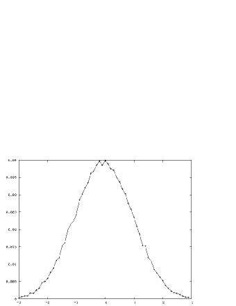
Figure 2: Testing the Normal Distribution

14 Omissions

SS intentionally omits certain features which are commonly found in spreadsheets and other computational environments. It omits data types other than simple strings and double precision floating point, targeting mainly numerical applications involving floating point operations. Internally, other data types may be used as appropriate when implementing specific algorithms, but the cell and symbol values are stored using floating point.

It also omits matrices and matrix operations, on the basis that applications requiring matrix operations are best implemented using one of the many existing high–quality commercial or free software packages designed for those kinds of applications.

15 Extensions

The current implementation of SS contains less than 40 numeric and range functions, which represent the most basic framework necessary for proof–of–concept. Most spreadsheets and programming environments contain hundreds of functions; for example, Gnumeric [6] contains 520, so any practical implementation must allow for easy extension by adding new functions.

The implementation of new internal functions should follow the same templates as user–defined functions,

the main difference being that internal functions are compiled–in whereas user–define functions are dynamically linked in at run–time. For example, the complete implementation of the irand function is:

/* 1 pseudo-random integer, 0<=irand(i)<=i-1
*/
double nf_irand(const Node *n, const Cell *c)
{
  int i = eval_tree( n->u.t.right, c);

  return (int) (i*(rand()/(RAND_MAX+1.0)));
}

By simply placing that code in an irand.c file in the numeric function sub–directory of the source code, it will be compiled–in. The first–line comment is used to specify how many arguments the function takes and a description that will be included in both the run–time help command and the documentation. The template for all functions consists of parse tree node and reference cell arguments, and a double return value.

16 Conclusion

The technical literature on spreadsheet implementation is relatively sparse [4], as opposed to publications covering use of spreadsheets. Innovation is hampered by requiring Excel compatibility and designing for non–programmer users. The computing environment proposed here brings together the spreadsheet and workspace (variables and symbol table) paradigms, with powerful batch input commands and C–compatible formula syntax. It provides flexibility in formula evaluation and range traversal, and allows cycles, so it can be used to implement iterative as well as traditional spreadsheet applications.

References

- [1] R. Perry, “Work in progress: Spreadsheet implementation programming project course,” in Frontiers in Education Conference, pp. T2H 13–418, Oct. 22–25, 2008.
- [2] B. Jelen, The Spreadsheet at 25. Holy Macro! Books, 2005.
- [3] R. Mattessich, Simulation of the Firm through a Budget Computer Program. Richard D. Irwin, Inc., 1964.
- [4] P. Sestoft, “A spreadsheet core implementation in C#.” www.itu.dk/ people/sestoft/corecalc/.
- [5] J. C. Bals, F. Christ, G. Engels, and M. Erwig, “Classsheets – model–based, object–oriented design of spreadsheet applications,” Journal of Object Technology, vol. 6, pp. 383–398, October 2007.
- [6] The Gnome Project, “Gnumeric spreadsheet.” projects.gnome.org/ gnumeric/.