Hubble Space Telescope reveals multiple Sub-Giant Branch in eight Globular Clusters111 Based on observations with the NASA/ESA Hubble Space Telescope, obtained at the Space Telescope Science Institute, which is operated by AURA, Inc., under NASA contract NAS 5-26555.
Abstract
In the last few years many globular clusters (GCs) have revealed complex color-magnitude diagrams, with the presence of multiple main sequences (MSs), broaden or multiple sub-giant branches (SGBs) and MS turn offs, and broad or split red giant branches (RGBs). After a careful correction for differential reddening, high accuracy photometry with the Hubble Space Telescope presented in this paper reveals a broadened or even split SGB in five additional Milky Way GCs: NGC 362, NGC 5286, NGC 6656, NGC 6715, and NGC 7089. In addition, we confirm (with new and archival HST data) the presence of a split SGB in 47Tuc, NGC 1851, and NGC 6388. The fraction of faint SGB stars with respect to the entire SGB population varies from one cluster to another and ranges from 0.03 for NGC 362 to 0.50 for NGC 6715. The average magnitude difference between the bright SGB and the faint SGB is almost the same at different wavelengths. This peculiarity is consistent with the presence of two groups of stars with either an age difference of about 1-2 Gyrs, or a significant difference in their overall C+N+O content.
1 Introduction
Recent photometric studies have revealed unexpectedly complex color-magnitude diagrams (CMDs) in many Globular Clusters (GCs), indicating that these stellar systems are not as simple as we have been assuming for decades (see Piotto 2009 for a recent review).
Centauri is the most famous example of a GC hosting complex multiple stellar populations. It has been known since the late nineties that its CMD shows multiple red-giant branches (RGBs, Lee et al. 1999, Pancino et al. 2000), sub-giant branches (SGBs e. g. Bellini et al. 2010) and multiple main sequences (MSs, Anderson et al. 1997, Bedin et al. 2004).
To date, multiple or broad RGBs have been observed in nearly all the GCs that have been observed with good signal-to-noise in the appropriate photometric bands (e. g. Marino et al. 2008, Yong et al. 2008, Lee et al. 2009, Lind et al. 2011). Recent studies also suggest that multimodal MSs could be quite common among GCs. In addition to the spectacular case of NGC 2808, which shows three distinct MSs (Piotto et al. 2007), double and triple MSs have been observed in several GCs, including NGC 104, NGC 6752, and NGC 6397 (Anderson et al. 2009, Milone et al. 2010, 2012a,b) and have been associated to stellar generations with a different content of helium and light-elements (e. g. Norris 2004, Piotto et al. 2005, D’Antona et al. 2005).
Also the CMDs of many stellar clusters in the Large and the Small Magellanic Cloud (LMC, SMC) are not consistent with single stellar populations (Bertelli et al. 2003, Mackey et al. 2008). Milone et al. (2009a) analyzed sixteen intermediate age clusters in the LMC and found that at least eleven of them (i.e. about the 70 % of the whole sample) exhibit a wide spread or a split around the main sequence turn-off (MSTO), which is consistent with the presence of multiple or prolonged star formation episodes.
Spectroscopic studies have long shown that most of the GCs exhibit some correlations and anticorrelations among light-element abundances (such as the Na-O anticorrelation, Kraft et al. 1979, 1994, Ramirez & Cohen 2002). The fact that light-element variations have also been observed among unevolved stars (e.g. Cannon et al. 1998, Gratton et al. 2001) indicates that they have a primordial origin (see Gratton et al. 2004 for a review).
However, it must be noted that spectroscopic analysis is necessarily limited to a small sample of (bright) stars, and therefore allows us to identify stellar generations which may constitute only a small fraction of the cluster populations. Often spectroscopy investigations cannot follow multiple stellar generations in all evolving sequences (in particular along the main sequence and the white dwarf cooling sequence). Information on multiple stellar generations is maximized when spectroscopic and photometric data can be used together. Otherwise, we must rely on photometry for a complete analysis of multiple populations (relative fraction, radial distribution, main chemical properties), which manifest themselves in different ways, in different clusters and different evolutionary parts of the CMD.
The multiple populations in NGC 1851 and NGC 104 manifest themselves most prominently in terms of a splitting of the SGB (Milone et al. 2008, 2012a, Anderson et al. 2009). NGC 6388 also shows hints of such a splitting as well (Piotto 2008 and Moretti et al. 2009). These SGB splits have been interpreted as indicating two groups of stars with either an age difference of about 1-2 Gyrs, or a significant difference in their overall C+N+O content (Cassisi et al. 2008, Ventura et al. 2009, Di Criscienzo et al. 2010).
In this paper we present detection of the broad (and most likely split) SGBs in five additional Milky Way GCs: NGC 362, NGC 5286, NGC 6656, NGC 6715, and NGC 7089, and confirm the presence of a double SGB in NGC 6388, NGC 104, and NGC 1851. In a companion paper based on the spectroscopy of stars selected from the CMDs published in this work, we have found that the two SGBs of NGC 6656 (M22) are made of stars with a different content of iron, -process elements, and C+N+O (Marino et al. 2012). A bimodality in -elements has been also observed along the RGB of NGC 1851 and associated with the double SGB of this cluster (e.g. Yong et al. 2008, Villanova et al. 2010, Lardo et al. 2012).
This paper is organized as follows. In Sect. 2 we describe the data set, the photometric reduction, the zero point calibrations, the selection of stars with high-quality photometry, and the differential-reddening correction. The initial detection of the SGB-broadenings is presented in Sect. 3. We then proceed to study the SGBs in increasing detail. We first use new and archival material: to derive proper motions to exclude field objects (Sect. 4) and to provide confirmation of the SGB-broadenings from several independent data-sets (Sect. 5). Section 6 then examines these SGBs through a variety of bandpasses. Finally, in Sect. 7, for each cluster we compare the fractions of stars in the different SGBs with the distribution of stars along the HB in hopes of identifying the same populations in the different evolutionary branches (Sect. 8). Section 9 contains the summary of results and an examination of open questions.
2 Observations and data reduction
We have used images taken with the Wide Field Planetary Camera 2 (WFPC2), the Wide Field Channel of the Advanced Camera for Surveys (WFC/ACS), and the ultraviolet and infrared channels of the Wide Field Camera 3 (UVIS and IR/WFC3) on board the Hubble Space Telescope (HST). These datasets include both proprietary images (GO11233, GO11739, GO12311, PI Piotto) and data that we retrieved from the STScI archive. In Table 1 we give a summary of the adopted data sets indicating: the cluster ID, the epoch of the observation, the number and the duration of the single exposures, the filters, the program ID, and the program PI.
The astrometry and photometry of WFPC2 images have been carried out for each chip, filter and epoch independently, by adopting the method described by Anderson & King (2000) based on the effective-point-spread function fitting. We corrected for the row error in HST’s WFPC2 cameras (see Anderson & King 1999 for details) and used the distortion solution as given by Anderson & King (2003). Photometric calibration has been done according to the Holtzman et al. (1995) Vega-mag flight system for the WFPC2 camera.
The astro-photometric reduction of ACS/WFC data was done with the software tools described in details by Anderson et al. (2008). It consists in a package that analyzes all the exposures of each cluster simultaneously in order to generate a single list of stars for each field. Stars are measured in each exposure with a library PSF that is “perturbed” to better match the PSF in that exposure. This routine was designed to work well in both crowded and uncrowded fields and it is able to detect almost every star that can be detected by eye. It takes advantage of the many independent dithered pointings of each image and the knowledge of the PSF to avoid including artifacts in the list. Calibration of ACS photometry into the Vega-mag system has been performed following recipes in Bedin et al. (2005) and using the zero points given in Sirianni et al. (2005). For ACS/WFC data coming from the GC Treasury program GO10775 (PI: Sarajedini) we simply used the calibrated catalogs produced by Anderson et al. (2008, see also Sarajedini et al. 2007) using the same procedures.
We measured star positions and fluxes on the WFC3 images with a software mostly based on img2xym_WFI (Anderson et al. 2006). Details on this program will be given in a stand-alone paper. Star positions and fluxes have been corrected for geometric distortion and pixel-area using the solutions provided by Bellini, Anderson & Bedin (2011) for WFC3/UVIS and Anderson et al. (in preparation) for WFC3/IR.
| ID | DATE | NEXPTIME | FILT | INSTRUMENT | PROGRAM | PI |
|---|---|---|---|---|---|---|
| NGC 362 | Dec 04 2003 | 2110s2120s | F625W | ACS/WFC | 10005 | Lewin |
| Dec 04 2003 | 4340s | F435W | ACS/WFC | 10005 | Lewin | |
| Sep 30 2005 | 370s20340s | F435W | ACS/WFC | 10615 | Lewin | |
| Jun 02 2006 | 10s4150s | F606W | ACS/WFC | 10775 | Sarajedini | |
| Jun 02 2006 | 10s4170s | F814W | ACS/WFC | 10775 | Sarajedini | |
| NGC 1851 | Nov 11-Dec 27 2010, Jan 2 2011 | 141280s | F275W | WFC3/UVIS | 12311 | Piotto |
| Nov 11-Dec 27 2010, Jan 2 2011 | 7100s | F814W | WFC3/UVIS | 12311 | Piotto | |
| Apr 10 1996 | 4900s | F336W | WFPC2 | 5696 | Bohlin | |
| May 01 2006 | 20s5350s | F606W | ACS/WFC | 10775 | Sarajedini | |
| May 01 2006 | 20s5360s | F814W | ACS/WFC | 10775 | Sarajedini | |
| NGC 5286 | Nov 07 1997 | 10s4140s | F555W | WFPC2 | 6779 | Gebhardt |
| Nov 07 1997 | 7s3140s | F814W | WFPC2 | 6779 | Gebhardt | |
| Mar 03 2006 | 30s5350s | F606W | ACS/WFC | 10775 | Sarajedini | |
| Mar 03 2006 | 30s5360s | F814W | ACS/WFC | 10775 | Sarajedini | |
| Mar 24 2009 | 60s3700s | F336W | WFPC2 | 11975 | Ferraro | |
| Mar 24 2009 | 2s3100s | F336W | WFPC2 | 11975 | Ferraro | |
| NGC 6388 | from Sep 04 2003 to Jun 26 2004 | 611s | F435W | ACS/WFC | 9821 | Pritzl |
| from Sep 02 2003 to Jun 23 2004 | 67s | F555W | ACS/WFC | 9821 | Pritzl | |
| from Oct 02 2003 to Jun 23 2004 | 63s | F814W | ACS/WFC | 9821 | Pritzl | |
| Apr 06 2006 | 40s5340s | F606W | ACS/WFC | 10775 | Sarajedini | |
| Apr 06 2006 | 40s5350s | F814W | ACS/WFC | 10775 | Sarajedini | |
| Apr 22-23 and May 17 2008 | 11700s11800s | F450W | WFPC2 | 11233 | Piotto | |
| Apr 22-23 and May 17 2008 | 11500s | F814W | WFPC2 | 11233 | Piotto | |
| Jun 30 and Jul 3 2010 | 6800s | F390W | WFC3/UVIS | 11739 | Piotto | |
| Jun 30 2010 | 6199s4249s | F160W | WFC3/IR | 11739 | Piotto | |
| NGC 6656 | Jun 06 2000 | 1226s | F555W | WFPC2 | 8174 | van Altena |
| Jun 06 2000 | 1126s | F785LP | WFPC2 | 8174 | van Altena | |
| Apr 01 2006 | 3s455s | F606W | ACS/WFC | 10775 | Sarajedini | |
| Apr 01 2006 | 3s465s | F814W | ACS/WFC | 10775 | Sarajedini | |
| Apr 29 2008 | 9350s | F450W | WFPC2 | 11233 | Piotto | |
| Apr 29 2008 | 9100s | F814W | WFPC2 | 11233 | Piotto | |
| Apr 22 2009 | 310s | F555W | WFPC2 | 11975 | Ferraro | |
| Apr 22 2009 | 3350s | F336W | WFPC2 | 11975 | Ferraro | |
| Sep 23 2010 and Mar 18 2011 | 9812s | F275W | WFC3/UVIS | 12311 | Piotto | |
| Sep 23 2010 and Mar 18 2011 | 450 | F814W | WFC3/UVIS | 12311 | Piotto | |
| NGC 6715 | Maj 25 2006 | 230s10340s | F606W | ACS/WFC | 10775 | Sarajedini |
| Maj 25 2006 | 230s10350s | F814W | ACS/WFC | 10775 | Sarajedini | |
| Jun 20-22-24 2007 | 9700s9800s | F450W | WFPC2 | 10922 | Piotto | |
| Jun 20-22-24 2007 | 9500s | F814W | WFPC2 | 10922 | Piotto | |
| Aug 30 1999 | 5300s350 | F555W | WFPC2 | 6701 | Ibata | |
| Aug 30 1999 | 260s5300s | F814W | WFPC2 | 6701 | Ibata | |
| NGC 7089 | Apr 16 2006 | 20s5340s | F606W | ACS/WFC | 10775 | Sarajedini |
| Apr 16 2006 | 20s4340s | F814W | ACS/WFC | 10775 | Sarajedini | |
| Aug 22 2000 | 600s2700s | F250W | WFPC2 | 8709 | Ferraro | |
| Aug 22 2000 | 250s500s2600s | F336W | WFPC2 | 8709 | Ferraro | |
| Jun 27 2008 | 10700s | F450W | WFPC2 | 11233 | Piotto | |
| Jun 27 2008 | 230s9200s | F450W | WFPC2 | 11233 | Piotto |
2.1 Selection of the star sample
Individual stars on the images may be poorly measured for several reasons: crowding by nearby neighbors, contamination from cosmic rays, or image artifacts, such as bad pixels, or diffraction spikes. The goal of the present work is to clearly identify multiple populations, which often manifest themselves as a splitting of 0.02 magnitudes or less in the cluster sequences. For this purpose we need to select the best-measured stars in the field (i.e. those with the lowest random and systematic errors), but we also need to have a large enough statistical sample to be able to identify secondary sequences that may have a much smaller fraction of stars than the primary ones.
The software described in Anderson et al. (2008) provides very valuable tools to reach this goal. In addition to the stellar fluxes and positions it generates a number of parameters that can be used as diagnostics of the reliability of photometric measurements. These include a parameter, , related to the quality of the fit of the PSF model to the star’s pixels, the difference in position for each star as measured in different filters, , the of magnitudes measured in different exposures, , and a parameter, , which quantifies how much a star is contaminated from neighboring stars flux (see Anderson et al. 2008 for the details).
To select the sample of stars with the best photometry, we adopted the following procedure, which is described in more details in Sect. 2.1 of Milone et al. (2009a). Since the and the parameters exhibit a trend with the magnitude, we divided the stars into bins of 0.04 magnitude and calculated for each bin the median of the and parameters and the percentile (hereafter ), by means of the iterative procedure explained in Milone et al. (2009a). We then added to the median of each bin four times and interpolated these points with a spline. All the stars that lie below the spline were flagged as well-measured. The parameter does not show a clear trend with magnitude, so we considered all the stars with as well-measured. In the cases of the most crowded clusters (namely NGC 5286, NGC 6388, NGC 6715, and NGC 7089) we have limited our investigation to stars with radial distance from the cluster center larger than 40 arcsec.
The fraction of stars that pass all the other criteria of selection, with respect to the total number of stars changes from one cluster to the other, and strongly depends on the dataset, and less critically on the luminosity of the star. As an example, in the case of NGC 6388, which is one the most crowded GCs of this paper, we have =0.66 for the F606W ACS/WFC GO10775 images and for stars brighter than . Specifically, 78% and 77% of the stars pass the criteria of selection based on the positions and magnitude respectively, 76% of stars pass the criteria based on the parameter, 78% that based on , and 66% all the criteria above. In the case of NGC6656, the most sparse GC in our sample, for F606W ACS/WFC images from GO10775 we have =0.89 for stars with .
2.2 Correction for differential reddening, and zero point spatial variations
The foreground reddening of the GCs studied in this paper goes from 0.05 (NGC 362) to 0.37 (NGC 6388, Harris 1996, 2010). Therefore, variations of reddening are expected within the field of view of our target clusters. Indeed, the CMDs in all clusters reveal that all the CMD sequences are significantly broader than what would be expected from our photometric precision, even taking into account the small unmodelable spatial changes of the PSF, which cause photometric zero-point variations usually smaller than 0.01 magnitude (see Anderson et al. 2008 for details).
Correcting for both differential reddening and the residual spatial variations of the photometric zero point represents a necessary step towards an accurate analysis of the cluster sequences. To obtain these corrections, we applied the method described in Milone et al. (2012c, Sect. 3). Briefly, we defined the fiducial MS for the cluster and estimated, for each star, how the observed stars in its vicinity may systematically lie to the red or the blue of the fiducial sequence; this systematic color and magnitude offset, measured along the reddening line, is indicative of the local differential reddening.
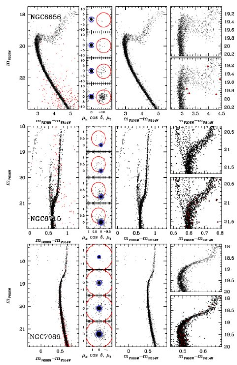
As an example, in the upper-left panel of Fig. 1 we plot the map of differential reddening in the field of view of NGC 6656. The CMD corrected for differential reddening is shown in the upper-right panel, while the original CMDs of stars in five, distinct 10001000 pixel regions are plotted in the lower panels. The fact that the double SGB is visible everywhere in the field of view further demonstrates that it cannot be an artifact introduced by differential reddening.
In Fig. 2 we show some CMDs before and after our differential-reddening correction for six out of the eight clusters considered in this work.

3 Multiple stellar populations along the SGB
Fig. 3 shows a zoom of the CMD region around the SGB for six of the clusters studied in this paper. Among the several data sets available for each cluster, we used here the ones with the best photometric quality for SGB stars. The most intriguing feature is already evident: the SGB is much broader than expected (indeed, in most cases split) from photometric errors, which are smaller than 0.01 mag for these selected stars. Note that the fraction of stars in the fainter SGBs differs from cluster to cluster, as discussed in detail in Sect. 7.
3.1 The multiple SGB of NGC 1851 and 47 Tucanæ
Excluding the peculiar case of Centauri, we now know from literature at least two additional GCs that show a SGB that is not consistent with a single stellar population222 We note that the SGB of NGC 6441 is also suspected to show two populations, but we postpone details and discussion to a forthcoming paper dedicated to the two anomalous GCs NGC 6388 and NGC 6441 (Bellini et al. 2012, in prep.) which will be based on HST program GO-11739..
The first is NGC 1851, which exhibits two clearly distinct SGB branches with a faint SGB containing about the 35 % of the SGB stars (Milone et al. 2008, 2009b).
The second is 47 Tuc, for which evidence of multiple stellar populations along the SGB of 47 Tuc came from the analysis of a large number of ACS/HST images by Anderson et al. (2009). These authors found that the SGB exhibits a clear spread in luminosity, with at least two distinct components: a brighter one with a significant spread in magnitude, and a second one about 0.05 mag fainter in the F475W band, containing about 10 % of the stars.
Milone et al. (2012a) found that the brighter SGB further splits into two branches, and that the presence of two stellar populations is clearly visible in the MS, RGB, and the HB.
These results have stimulated us to start a deeper investigation using the WFC3/UVIS camera: GO-12311 (PI Piotto). The versus CMD of NGC 1851, obtained combining these data and archive ones, is shown in Fig. 4. This CMD not only confirms the presence of a split SGB, but it is so far the clearest bi-modal SGB in literature.
In Fig. 5 we reproduce Fig. 12 from Milone et al. (2012a), which shows the complex SGB of 47 Tuc. In the versus we see the faint SGB discovered by Anderson et al. (2009) (these stars are colored red). The versus and the versus CMDs are plotted in the middle and the right panel and show the other two SGB branches.

Table LABEL:parameters shows the relevant (for the present paper) parameters for the eight GCs with a significant SGB broadening, and that we will discuss in the following. Most of them come from Harris (1996, updated as in 2010). HBR is the Horizontal Branch ratio HBR=(B-R)/(B+V+R), where B, R, and V are the numbers of blue HB, red HB and RR Lyrae (from Harris 1996, updated as in 2010). The HBR for NGC 6388 has been calculated from the CMD presented in here.
| ID | HBR | [Fe/H] | ||||
|---|---|---|---|---|---|---|
| NGC 104 | 7.4 | 0.04 | 13.37 | 0.99 | 9.42 | 0.76 |
| NGC 362 | 9.4 | 0.05 | 14.81 | 0.87 | 8.41 | 1.16 |
| NGC 1851 | 16.7 | 0.02 | 15.47 | 0.36 | 8.33 | 1.22 |
| NGC 5286 | 8.4 | 0.24 | 15.95 | 0.24 | 8.61 | 1.67 |
| NGC 6388 | 3.2 | 0.37 | 16.14 | 0.63 | 9.42 | 0.60 |
| NGC 6656 | 4.9 | 0.34 | 13.60 | 0.91 | 8.50 | 1.76 |
| NGC 6715 | 19.2 | 0.15 | 17.61 | 0.75 | 10.1 | 1.58 |
| NGC 7089 | 10.4 | 0.06 | 15.49 | 0.96 | 9.02 | 1.62 |
4 Proper motions
The stellar fields analyzed in this paper are all located within few arcminutes from the cluster centers. As a consequence, in all the cases, the number of field stars is negligible with respect to the cluster members. However, while in NGC 5286, NGC 6388, NGC 6656, NGC 6715 both SGBs are well populated, and therefore well distinguishable from field stars, in NGC 362 and NGC 7089 the faint SGB (fSGB) contains only a small fraction of the total number of SGB stars. For these two clusters, the effect of the field contamination is more relevant for the assessment of the significance of the fSGB. One of the most obvious advantages of having more than one epoch observations is the possibility to measure the proper motions of stars. In the following, we use proper motions to show that in all clusters, both the fSGB and bright SGB (bSGB) belong to the cluster, and cannot be associated to field-stars.
For NGC 362, NGC 5286, NGC 6388, NGC 6656, and NGC 7089, we have used the proper-motion measurements from Milone et al. (2012c). For NGC 6715 we determined proper motions from GO6701 (hereafter epoch 1), GO10775 (epoch 2) and GO10922 (epoch 3) data. To do this, we followed the procedure that has been used for the other clusters by McLaughlin et al. (2006), Bedin et al. (2009), and Anderson & van der Marel (2010).
Briefly, we have adopted as reference frames the frames defined by Anderson et al. (2008) for GO10775 data set, which have increasing from east to west, and from south to north. We corrected for distortion the coordinates of each star measured in each exposure, and transformed the average position for each star in each of the three epochs into the master frame (, i=1,2,3).
To minimize the effects of any residual distortion, we applied local transformations using a local subsample of stars. To determine the transformation for each star, we selected the closest stars to the target star as local reference stars. The corresponding 55 pairs of coordinates in the two frames are used to determine the least-squares linear transformation from one coordinate system to the other. Naturally, we excluded the target star in its own transformation.
We used linear transformations in the form:
| (1) |
| (2) |
where , i=1,2,3 are the coordinates of the target stars in the distortion-corrected master-frame, while , i=1,2,3 are those in the non-reference frames, and the constants ,,,, (, ), and (, ) are to be determined.
Finally we plotted the positions of the star along and as a function of the epoch expressed in years and obtained the motion components on the plane of the sky by standard, error-weighted least squares fit of a straight line to the points, allowing both the slope and the zero point to vary. The best estimate of stellar proper motions (in pixels per year) is given by the slope of the line multiplied by the pixel-scale of the reference frame which is 49.7248 mas/pixel (van der Marel et al. 2007).
The selection of the reference stars is crucial for accurate transformations. Therefore, we imposed that reference stars must be unsaturated in the images of both epochs, and must pass the criteria of selection described in Sect. 2.
We further note that the internal proper-motions of cluster stars are usually negligible with respect to our errors333 An exception is represented by the nearby GCs M 22, where the internal cluster velocity dispersion is significantly larger than the proper-motion errors but at least five times smaller than field star proper motion.. Therefore, we can refer our motions to the bulk of cluster members motion. In order to select a pure sample of cluster members, we started by identifying all the stars that, on the basis of their position in the CMD, are probable cluster members and obtained a crude proper-motion estimate by using a local transformation based on this sample. Then we have iteratively excluded from this list all the stars that did not have cluster-like proper motions (proper motion , where is the proper-motion dispersion of cluster members), despite their proximity to the cluster sequences. This ensures that the relative motions of cluster stars should be, on average, zero.
Results (and proper-motion-selection criteria) are shown in Figs 6-7. In the left panel we show the CMD for all the stars for which proper-motion measurements are available. The second column of the panels shows the proper-motion diagrams of the stars for four different magnitude intervals. The blue and red circles are drawn in order to select two groups of stars that have member-like and field stars-like motions, respectively. The red circle size has been chosen by eye with the criterion of rejecting the most evident field stars that are plotted in red in the left panel CMD.
It should be noted that in our study it is more important to have a pure cluster sample than a complete one. Therefore, we fixed the radius of blue circles at 2.5 , where is the proper-motion dispersion in each dimension. If we assume that proper motions of cluster stars follow a bivariate Gaussian distribution, each circle should include 95 % of the cluster members in each magnitude interval. The third column panels show the CMD of our chosen cluster stars, and the rightmost upper panel is a blowup of the CMD region around the SGB. In the rightmost lower panel we marked in black the location of stars with cluster like motion, and in red field stars. In all cases, the stars in both the fSGB and bSGB regions have cluster-like proper motion and cannot be attributed to a field population.
5 Confirming the split/spread SGB with independent datasets
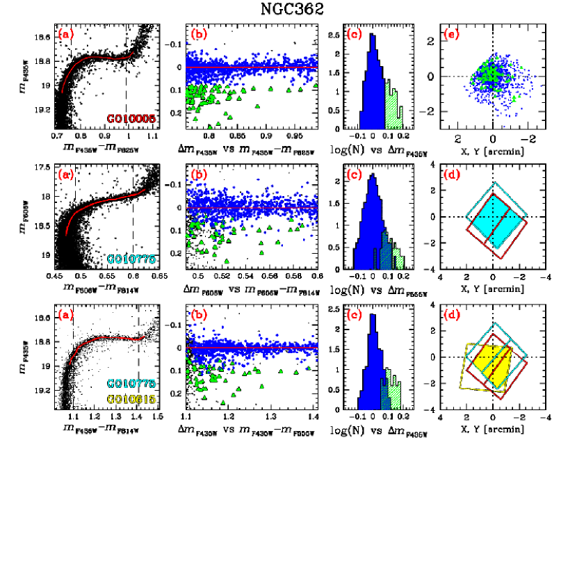
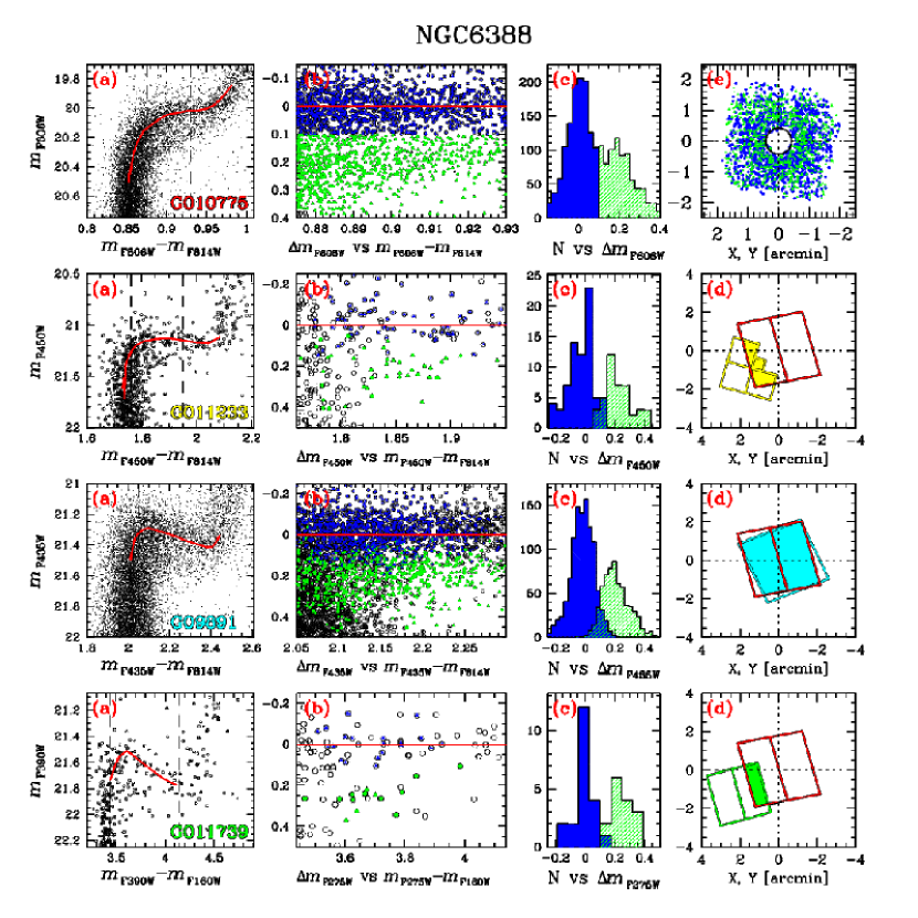
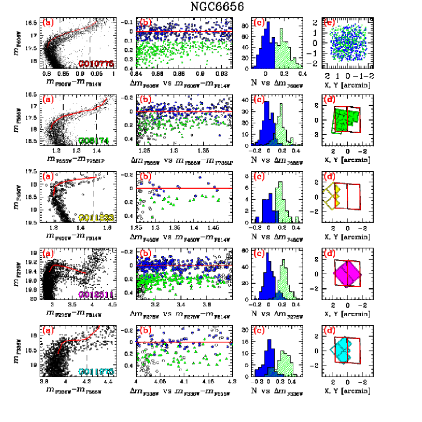
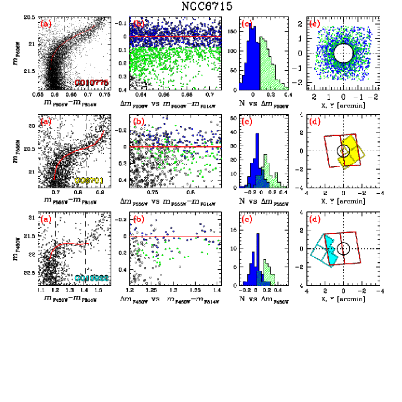
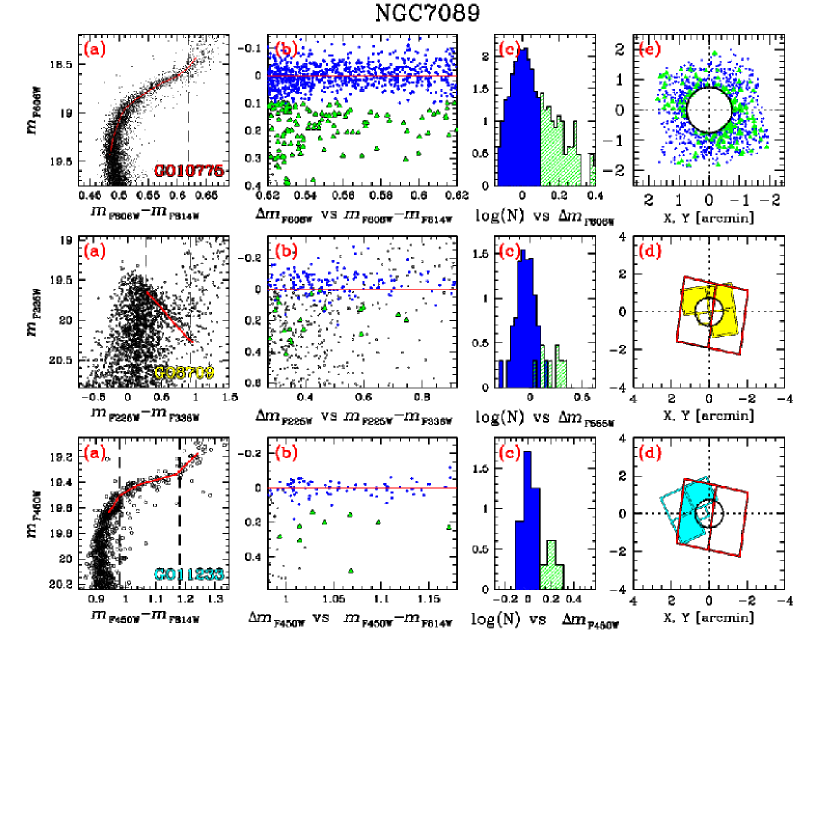
In this section we make use of a larger set of HST photometry to further confirm and study the SGB spread identified in Fig. 3. Figures 8 through 13 present the multi-filter analysis for 6 out of the eight clusters considered in this work; we describe the procedure in detail here for NGC 362. Panels a of Fig. 8 show the three CMDs of NGC 362 that can be constructed from the three independent data sets we have available. The red line overplotted on each CMD is a fiducial line drawn by hand. We have also calculated the magnitude difference () between each star and the fiducial line and plotted it (in panels b) as a function of color, for stars in the color interval delimited by the dashed lines of panels a.
In the top panel b, we divided the SGB as seen in F475W-versus-(F435WF625W) from GO-10005 into two groups based on the F435W magnitude, and colored the bSGB stars blue and the fSGB stars green. Note that the choice of the two groups of stars is arbitrary, and it is not intended to demonstrate that these two groups correspond to two distinct SGBs. The intent here is to demonstrate that the SGB spread is real and significant, in all clusters. In all the other panels we used this color-coding for the same stars. The fact that the green stars lie systematically below the main SGB in all the plots demonstrates that they are indeed intrinsically fainter.
The histograms in panels c show the distribution in each different CMD. The fact that the median of fSGB and bSGB stars differs by 7 444 We indicate with the error associated with as the ratio between the color dispersion measured for all the stars in a given SGB component and the square-root of their number minus one. in all the independent data sets demonstrates that the observed spread is real. Panels d show the footprints of the various comparison data sets relative to the cluster center. Only stars in the shaded region are used in the analysis presented. Stars within the black circles (where present, for example in NGC 5286) have poor photometric quality because of crowding, and are excluded from our analysis. The spatial distribution of bSGB and fSGB stars is shown in the uppermost right panel e.

6 A multi-wavelength analysis of the SGB split/spread
Recent studies have demonstrated that the our ability to detect multiple RGB and MS sequences in globular clusters can be very sensitive to the particular filter system used to study them. For example, the RGBs of both NGC 6121 and NGC 6752 are clearly bimodal in the U vs. UB CMD, yet there is no evidence for any split or intrinsic color spread of the RGB when they are observed in the BI color (Marino et al. 2008). Similar multiple RGBs have been also observed in CMDs made with the corresponding Strömgren filters (e.g. Grundahl 1999, Yong et al. 2008). These RGB splits have been interpreted as being related to how CN, CH, and NH bands affect some spectral regions, but not others (Marino et al. 2008, Yong et al. 2008). Similarly, the color differences between the multiple MSs of Centauri, 47 Tucanæ, NGC 6397, and NGC 6752 depend strongly on the particular color baseline used to study them. These MS splits have been attributed to a bimodal distribution in helium abundance.
In this section we take advantage of the huge photometric dataset available for each cluster in order to investigate how the SGB morphology changes from filter system to filter system. Although each of our clusters has been observed in a different set of bands, each cluster has enough wavelength coverage to make direct comparisons possible.
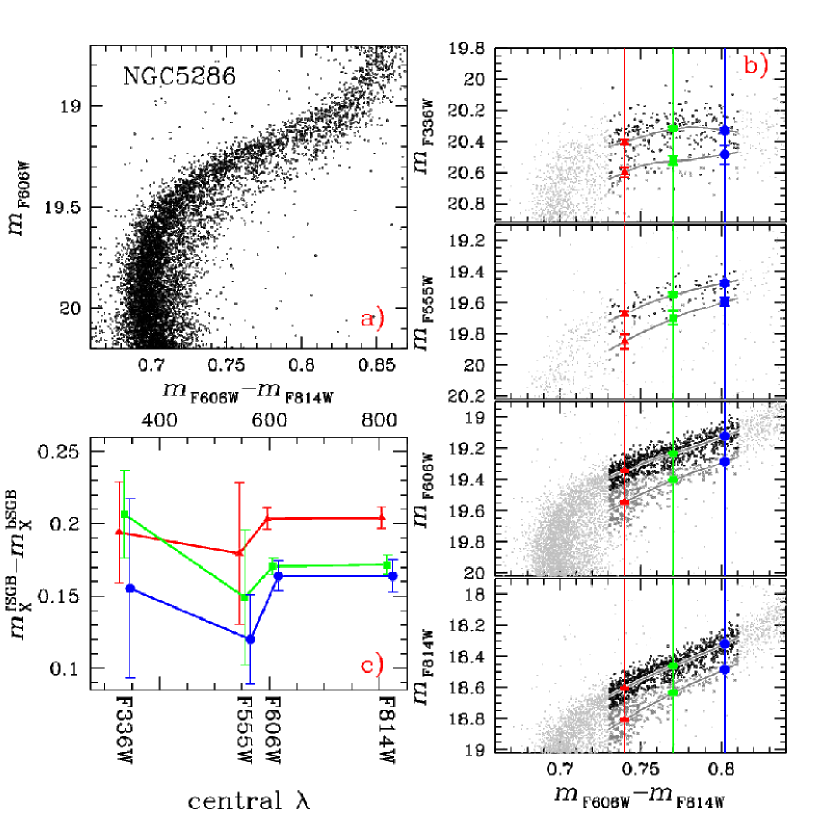
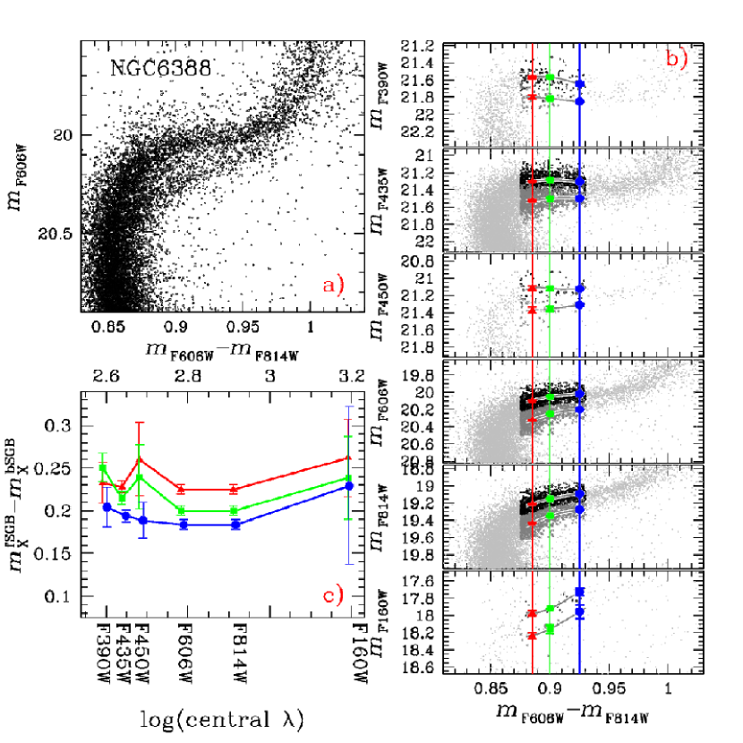
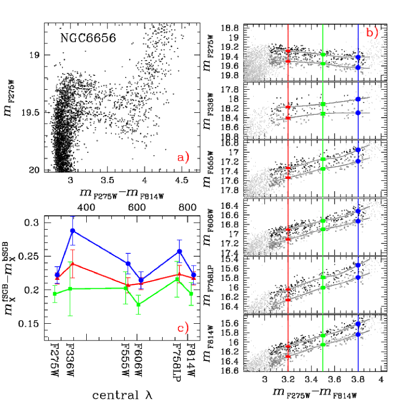
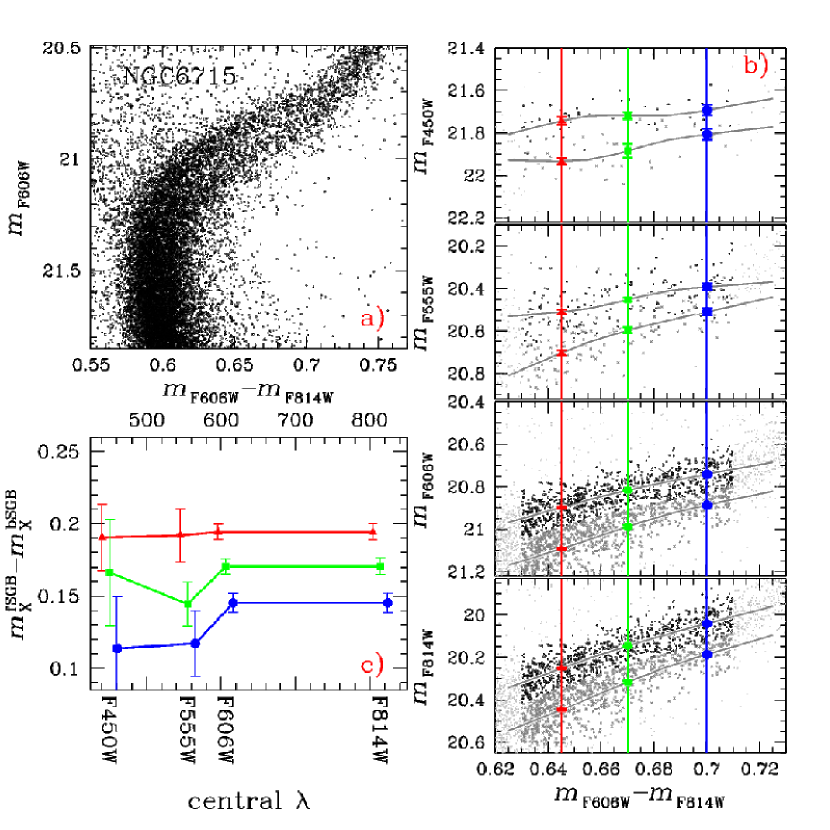
The approach we use here is similar to our study of the MS in Centauri (Bellini et al. 2010). Our aim will be to trace out the fiducial sequences for the two SGBs in multiple filter bands and quantify the offset between the sequences as a function of color at a set of points across the SGB. If this difference is relatively constant with wavelength, then it is indicative of a difference in the stellar structure (i.e. , radius) for the stars in the two sequences. On the other hand, if the difference varies with wavelength, then there could be atmospheric effects going on as well.
Our approach is illustrated in Fig. 14 for NGC 1851. For this cluster, we have observations for the same stars through the F275W, F336W, F606W, and F814W filters. In the upper left panel (a), we show the stars in the color system that best separates the populations. For this cluster, that is in F275W versus F275WF814W.
We associate each star along the SGB with either the bright or the faint population. In the panels on the right (b), we color-code the stars by population and plot them in the same color system (F275WF814W), but with a different photometric band along the vertical axis in each panel. The upper SGB is shown as black points and the lower SGB as medium gray points. We then trace out the upper and lower sequences by specifying a set of fiducial points along each of them.
Finally we measured the magnitude difference between the fiducial line of the faint and the bright sequences corresponding to the three colors indicated by the blue, green, and red line. We plot the difference between the faint and bright sequences in each photometric band in the lower-left panel (c) for each color. The error bars are indicative of the number and spread of the points that went into the value plotted. It is clear that the separation between the sequences is relatively constant with photometric band and it is also relatively the same for all three groups.
In Figures 15-18, we perform the same analysis for NGC 5286, NGC6388, NGC 6656, NGC 6715. We have excluded from this analysis NGC 362 and NGC 7089 because the small number of stars in the fSGB does not allow us to obtain a fully realiable fiducial line. All of these show roughly the same behavior: the magnitude difference between the bSGB and the fSGB has almost no dependence on wavelength. This behavior rules out the hypothesis that the observed SGB split could be related to some effects due to molecular bands on the atmosphere (which would affect only specific photometric filters), in contrast to what has been seen on the RGB. Rather it must be due to some difference in the stellar structure (or mass).
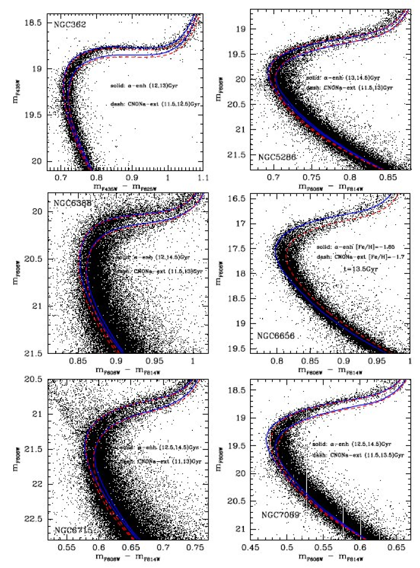
We will defer a detailed comparison of our CMDs with theoretical isochrones to a dedicated paper, but it is worth mentioning here that these general results are very similar to what has already been found for NGC 1851 by Cassisi et al. (2008) and Ventura et al. (2009). In particular:
-
•
If we assume that the two stellar populations represented by the two SGBs have the same – -enhanced – chemical composition and that the SGB split (or magnitude dispersion) is due to an age difference alone, stars populating the fSGB should be older by 1-2 Gyrs.
-
•
Alternatively, if the bSGB and the fSGB stars have different chemical compositions, with the fSGB stars being CNO-enriched, the stellar groups corresponding to the two SGBs could be – when accounting for the quoted uncertainty on the relative age – nearly coeval, or the fSGB could be slightly younger.

For the clusters analized above we found that the SGBs can be characterized being as bimodal or broad in every filter system. This is in contrast to the well-studied case of 47 Tuc, which has been shown to have two close upper SGBs and a more separated lower SGB. In 47 Tuc, we were able to follow the two populations through the entire CMD, from the MS to the SGB, RGB, and HB.
Even though 47 Tuc clearly has a more complicated morphology than these clusters, since the sequences have been studied both photometrically and spectroscopically, it yet may help us understand the simpler phenomenon at work here. In 47 Tuc, the two upper SGBs contain 92% of the stars at the center. The more populous upper sequence (hereafter mSGB) has been shown to consist of CN-strong/Na-rich/O-poor stars, while the less populous sequence (uSGB) is made up of CN-weak/Na-poor/O-rich stars. The lowest SGB (named lSGB) also appears to be CN-strong/Na-rich/O-poor, like the mSGB (Milone et al. 2012a).
In order to compare the SGB of 47 Tuc with these clusters, in Fig. 19 we adapt the procedure introduced in Fig. 14 for NGC 1851, to the triple SGB of 47 Tuc. In the CMDs of left panels, the sample of uSGB, mSGB, and lSGB stars selected by Milone et al. (2012a) are colored green, magenta, and red, respectively. Similar to what was done for NGC 1851, we have calculated for each CMD the magnitude difference between the mSGB and the uSGB, between the lSGB and the uSGB, and between the lSGB and mSGB the at the color levels indicated by the three vertical lines. In the left panels we again plotted these magnitude differences as a function of the central wavelength of the different bands in our dataset. We found that the lSGB is about 0.05 magnitude fainter than the mSGB, as indicated by the filled symbols, and that this magnitude difference is the same, within our error bars, at all wavelengths, similar to what we found for the other clusters studied in this paper. The uSGB is typically 0.02 mag brighter than the mSGB and 0.08 magnitude brighter than the lSGB, but their magnitude separation increases to 0.08 mag and 0.14 mag in the F336W band (open symbols), respectively. Since the F336W filter includes the NH molecular bands at 3300Å, we suggest that the latter behavior is due to a higher N content (strong NH band absorption) in mSGB stars.
These results support the findings of Di Criscienzo et al. (2010) and Milone et al. (2012a). According to these authors, the implication is that the uSGB must correspond to the first stellar population with a chemical composition similar to the halo stars, while the mSGB should be made by N/Na/He-rich O/C-poor second-generation stars. Only a small fraction of the second generation is also characterized by an overall C+N+O increase: these stars represent the lSGB.

7 Population ratio
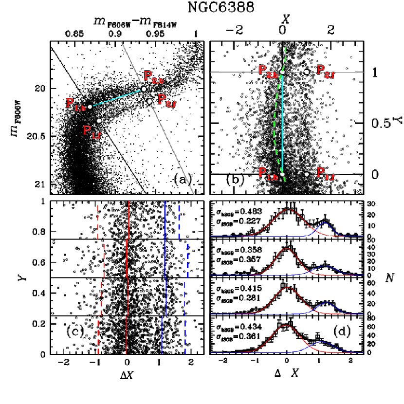
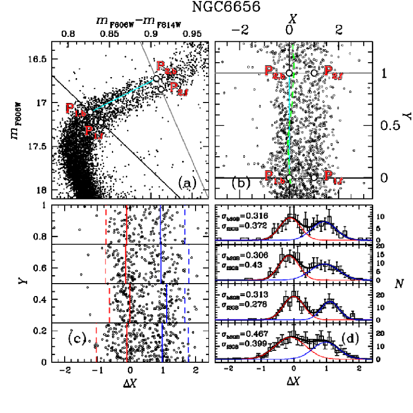
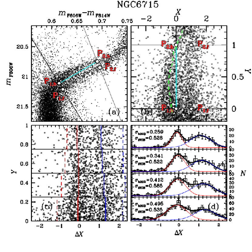
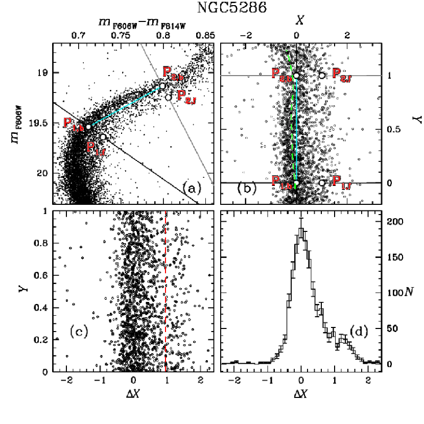
The fractions of stars in the different generations can provide fundamental constraints on the formation and evolution of these stellar systems. To estimate the numbers of fSGB and bSGB stars, we adopted a procedure similar to the one used by Milone at al. (2009b), and illustrated in Figures 20- 25 for six of the clusters studied in this paper.
Briefly, we selected by hand two points on the fSGB (, ) and the bSGB (, ) with the purpose of delimiting the SGB region where the split is most evident, as shown in panel a. These two points have been connected with a straight line, as shown in panel a. Only stars contained within the region between these lines were used in the following analysis. In panel b we have transformed the CMD into a reference frame where the origin corresponds to ; has coordinates (1,0), and the coordinates of and are (0,1) and (1,1), respectively. As in Milone et al. (2009b), in the following, we indicate as ‘X’ and ‘Y’ the abscissa and the ordinate of this reference frame. The dashed green line is the fiducial line of the bSGB.
In panel c we have calculated the difference between the X value of each star and the X of the fiducial line ( X). In the cases of NGC 6388, NGC 6656, and NGC 6715 the histograms in panel d are the X distribution for stars in four Y intervals (see Figs. 20-22). These distributions have been modeled as the sum of two partially overlapping Gaussian functions. In the cases of NGC 362, NGC 5286, and NGC 7089, where the number of fSGB stars is too small not only to fit with an independent Gaussian, but also to distinguish if the fSGB and the bSGB are two distinct populations or the product of continuous star-formation epishodes. we have arbitrarily drawn the vertical line in panel c to separate the groups of fSGB and bSGB stars (see Figs. 23-25).
It is important to note that each of the points , , , and — arbitrarily defined with the sole purpose of isolating a group of stars representative of each of the two SGBs—corresponds to a different mass (, , , and ). To obtain a reliable measure of the fraction of stars in each of the two populations (hereafter: , ) we have to compensate for the fact that the two stellar groups that define the two SGBs cover two different mass intervals (), due to the different evolutionary lifetimes. Consequently, the correction we have to apply will be somewhat dependent on the choice of the mass function, .
To this end, we can calculate the fraction of stars in each branch as:
where , are the observed numbers of stars, the adopted mass function, and and the areas under the Gaussians, for the bSGB and fSGB stars. The latter are calculated as the areas of the Gaussians that best fit the bSGB and the fSGB in the cases of NGC 6388, NGC 6656, and NGC 6715, while for NGC 362, NGC 5286, and NGC 7089 we assumed that and correspond to the number of stars on the blue and the red side of the dashed line of panel c.
As for the dependence on the adopted mass function, we ran the following test. We assumed first an heavy-mass-dominated mass function () and a then steep () mass function. Even with these extreme assumptions, we found that the mass function effect can change the relative fSGB/bSGB population ratio by a negligible 3%. Therefore, for simplicity, we adopted a Salpeter (1955) IMF for .
Results are listed in Table 3. Columns 2 and 3 list the relative number of each population obtained by assuming that the two SGBs have the same age but different C+N+O content (fSGB stars with two times more C+N+O than bSGB ones). The relative number of bSGB and fSGB stars listed in Cols. 4 and 5 are calculated by assuming for the two SGBs the same overall CNO but different age ( age Gyr, fSGB older, Fig. 26, see Cassisi et al. 2008). We found that by using the different isochrones the resulting fractions of fSGB and bSGB stars changes by less than 0.04. In most cases these differences are within our uncertainties.
We found that in five out of six GCs in Table 3 the bSGB contains the majority of the cluster stars, which is also what has been observed in NGC 104 (Anderson et al. 2009) and NGC 1851 (Milone et al. 2009b), bringing the statistics to seven out of eight. The fraction of fSGB and bSGB varies considerably from cluster to cluster: it is a few percent in the cases of NGC 362 and NGC 7089 and 50% for the case of NGC 6715.


| Same age, twice C+N+O | Same C+N+O, age 1-2 Gyr | |||
|---|---|---|---|---|
| ID | ||||
| NGC 362 | 0.970.01 | 0.030.01 | 0.990.01 | 0.010.01 |
| NGC 5286 | 0.870.03 | 0.130.03 | 0.850.03 | 0.150.03 |
| NGC 6388 | 0.780.02 | 0.220.02 | 0.900.02 | 0.100.02 |
| NGC 6656 | 0.600.04 | 0.400.04 | 0.560.04 | 0.360.04 |
| NGC 6715 | 0.470.04 | 0.530.04 | 0.490.04 | 0.510.04 |
| NGC 7089 | 0.950.01 | 0.050.01 | 0.970.01 | 0.030.01 |
8 Summary
In this paper we have shown that the Galactic GCs NGC 362, NGC 5286, NGC 6388, NGC 6656, NGC 6715, and NGC 7089, exhibit double or broadened SGBs, similar to those identified in NGC 1851 (Milone et al. 2008) and NGC 104 (Anderson et al. 2009, Milone et al. 2012a). When we compare different CMDs of the same cluster made with different magnitudes and color combinations, we find that the magnitude difference between the bright and the faint SGB components remains approximately constant and does not depend on the used filters. Therefore, we conclude that the split/spread SGB of the GCs studied in this paper can be interpreted in terms of two stellar groups with either a difference in age by 1-2 Gyr or a large difference in the total C+N+O abundance, as previously suggested by Cassisi et al. (2008) and Ventura et al. (2009) for the case of NGC 1851. In the cases of NGC 362, NGC 7089, and NGC 5286, the small number of fSGB stars do not allow us to firmly estabilish if the two groups of fSGB and bSGB stars correspond to two distinct stellar populations or if the poorly populated fSGBs are just the tail of an exthended star-formation history.
The fractions of faint and bright SGB stars with respect to the total number of SGB stars changes from cluster to cluster, and ranges from (0.03:0.97) in the case of NGC 362 to (0.51:0.49) for the Sagittarius dwarf galaxy’s GC NGC 6715.
References
- Anderson (1997) Anderson, A. J. 1997, Ph.D. Thesis,
- Anderson & King (1999) Anderson, J., & King, I. R. 1999, PASP, 111, 1095
- Anderson & King (2000) Anderson, J., & King, I. R. 2000, PASP, 112, 1360
- Anderson & King (2003) Anderson, J., & King, I. R. 2003, PASP, 115, 113
- Anderson & King (2006) Anderson, J., & King, I. R. 2006, ACS ISR 2006-01
- Anderson et al. (2006) Anderson, J., Bedin, L. R., Piotto, G., Yadav, R. S., & Bellini, A. 2006, A&A, 454, 1029
- Anderson et al. (2008) Anderson, J., Sarajedini, A., Bedin, L. R., et al. 2008, AJ, 135, 2055
- Anderson et al. (2009) Anderson, J., Piotto, G., King, I. R., Bedin, L. R., & Guhathakurta, P. 2009, ApJ, 697, L58
- Anderson & van der Marel (2010) Anderson, J., & van der Marel, R. P. 2010, ApJ, 710, 1032
- Bedin et al. (2004) Bedin, L. R., Piotto, G., Anderson, J., et al. 2004, ApJ, 605, L125
- Bedin et al. (2005) Bedin, L. R., Cassisi, S., Castelli, F., et al. 2005, MNRAS, 357, 1038
- Bellini et al. (2010) Bellini, A., Bedin, L. R., Piotto, G., et al. 2010, AJ, 140, 631
- Bellini et al. (2011) Bellini, A., Anderson, J., & Bedin, L. R. 2011, PASP, 123, 622
- Bellini et al. (2012) Bellini, A., Piotto, G., Milone, A. P. et al. 2012, in preparation
- Bertelli et al. (2003) Bertelli, G., Nasi, E., Girardi, L., et al. 2003, AJ, 125, 770
- Cannon et al. (1998) Cannon, R. D., Croke, B. F. W., Bell, R. A., Hesser, J. E., & Stathakis, R. A. 1998, MNRAS, 298, 601
- Cassisi et al. (2008) Cassisi, S., Salaris, M., Pietrinferni, A., et al. 2008, ApJ, 672, L115
- D’Antona et al. (2005) D’Antona, F., Bellazzini, M., Caloi, V., et al. 2005, ApJ, 631, 868
- di Criscienzo et al. (2010) di Criscienzo, M., Ventura, P., D’Antona, F., Milone, A., & Piotto, G. 2010, MNRAS, 408, 999
- Grundahl (1999) Grundahl, F. 1999, Spectrophotometric Dating of Stars and Galaxies, 192, 223
- Holtzman et al. (1995) Holtzman, J. A., Burrows, C. J., Casertano, S., et al. 1995, PASP, 107, 1065
- Kraft (1979) Kraft, R. P. 1979, ARA&A, 17, 309
- Kraft (1994) Kraft, R. P. 1994, PASP, 106, 553
- Lardo et al. (2012) Lardo, C., Milone, A. P., Marino, A. F., et al. 2012, A&A, 541, A141
- Lee et al. (1999) Lee, Y.-W., Joo, J.-M., Sohn, Y.-J., et al. 1999, Nature, 402, 55
- Lee et al. (2009) Lee, J.-W., Kang, Y.-W., Lee, J., & Lee, Y.-W. 2009, Nature, 462, 480
- Lind et al. (2011) Lind, K., Charbonnel, C., Decressin, T., et al. 2011, A&A, 527, A148
- Mackey et al. (2008) Mackey, A. D., Broby Nielsen, P., Ferguson, A. M. N., & Richardson, J. C. 2008, ApJ, 681, L17
- Marino et al. (2008) Marino, A. F., Villanova, S., Piotto, G., et al. 2008, A&A, 490, 625
- Marino et al. (2009) Marino, A. F., Milone, A. P., Piotto, G., et al. 2009, A&A, 505, 1099
- Marino et al. (2012) Marino, A. F., Milone, A. P., Sneden, C., et al. 2012, A&A, 541, A15
- McLaughlin et al. (2006) McLaughlin, D. E., Anderson, J., Meylan, G., et al. 2006, ApJS, 166, 249
- Milone et al. (2008) Milone, A. P., Bedin, L. R., Piotto, G., et al. 2008, ApJ, 673, 241
- Milone et al. (2009) Milone, A. P., Bedin, L. R., Piotto, G., & Anderson, J. 2009a, A&A, 497, 755
- Milone et al. (2009) Milone, A. P., Stetson, P. B., Piotto, G., et al. 2009b, A&A, 503, 755
- Milone et al. (2010) Milone, A. P., Piotto, G., King, I. R., et al. 2010, ApJ, 709, 1183
- Milone et al. (2012) Milone, A. P., Piotto, G., Bedin, L. R., et al. 2012a, ApJ, 744, 58
- Milone et al. (2012) Milone, A. P., Marino, A. F., Piotto, G., et al. 2012b, ApJ, 745, 27
- Milone et al. (2012) Milone, A. P., Piotto, G., Bedin, L. R., et al. 2012c, A&A, 540, A16
- Moretti et al. (2009) Moretti, A., Piotto, G., Arcidiacono, C., et al. 2009, A&A, 493, 539
- Norris (2004) Norris, J. E. 2004, ApJ, 612, L25
- Pancino et al. (2000) Pancino, E., Ferraro, F. R., Bellazzini, M., Piotto, G., & Zoccali, M. 2000, ApJ, 534, L83
- Piotto et al. (2005) Piotto, G., Villanova, S., Bedin, L. R., et al. 2005, ApJ, 621, 777
- Piotto et al. (2007) Piotto, G., Bedin, L. R., Anderson, J., et al. 2007, ApJ, 661, L53
- Piotto (2008) Piotto, G. 2008, Mem. Soc. Astron. Italiana, 79, 334
- Piotto (2009) Piotto, G. 2009, IAU Symposium, 258, 233, arXiv:0902.1422
- Ramírez & Cohen (2002) Ramírez, S. V., & Cohen, J. G. 2002, AJ, 123, 3277
- Salpeter (1955) Salpeter, E. E. 1955, ApJ, 121, 161
- Sarajedini et al. (2007) Sarajedini, A., Bedin, L. R., Chaboyer, B., et al. 2007, AJ, 133, 1658
- Sirianni et al. (2005) Sirianni, M., Jee, M. J., Benítez, N., et al. 2005, PASP, 117, 1049
- Ventura et al. (2009) Ventura, P., Caloi, V., D’Antona, F., et al. 2009, MNRAS, 399, 934
- Villanova et al. (2010) Villanova, S., Geisler, D., & Piotto, G. 2010, ApJ, 722, L18
- Yong et al. (2008) Yong, D., Grundahl, F., Johnson, J. A., & Asplund, M. 2008, ApJ, 684, 1159
- Yong & Grundahl (2008) Yong, D., & Grundahl, F. 2008, ApJ, 672, L29