Scaling Multiple-Source Entity Resolution using
Statistically Efficient Transfer Learning

Abstract

We consider a serious, previously-unexplored challenge facing almost all approaches to scaling up entity resolution (ER) to multiple data sources: the prohibitive cost of labeling training data for supervised learning of similarity scores for each pair of sources. While there exists a rich literature describing almost all aspects of pairwise ER, this new challenge is arising now due to the unprecedented ability to acquire and store data from online sources, features driven by ER such as enriched search verticals, and the uniqueness of noisy and missing data characteristics for each source. We show on real-world and synthetic data that for state-of-the-art techniques, the reality of heterogeneous sources means that the number of labeled training data must scale quadratically in the number of sources, just to maintain constant precision/recall. We address this challenge with a brand new transfer learning algorithm which requires far less training data (or equivalently, achieves superior accuracy with the same data) and is trained using fast convex optimization. The intuition behind our approach is to adaptively share structure learned about one scoring problem with all other scoring problems sharing a data source in common. We demonstrate that our theoretically motivated approach incurs no runtime cost while it can maintain constant precision/recall with the cost of labeling increasing only linearly with the number of sources.

1 Introduction

In this paper we investigate a serious and previously-unexplored challenge to scaling joint entity resolution (ER) to multiple sources: that of intractable labeling costs required to model heterogeneities in real-world data sources.

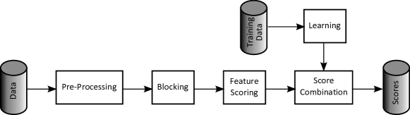
Figure 1: A typical ER data flow. This paper focuses on the learning step, under multiple data sources, that infers the similarity of each pair of entities from attribute similarities, based on human-labeled examples of matching and non-matching record pairs.

Significant attention has already been focused on ER in the DB, data mining and statistics communities, where the typically-stated goals are computational performance (good runtime) and statistical performance (good precision/recall)—cf. e.g., [18, 13] and references therein for general discussions on ER. The most common approach for achieving good precision/recall is to employ supervised learning to combine domain-expert-selected feature scores into overall similarity scores [17, 35, 18, 26, 4, 32, 28, 25, 9]. Indeed a recent, comprehensive evaluation of over 20 state-of-the-art ER systems [19], Köpcke et al.found that on most tasks supervised learning-based matchers offer superior performance.

However Köpcke et al.also noted that statistical performance comes at the price of human effort in labeling training examples, and explicitly highlight labeling cost as a key measure of matcher performance. But while there have been studies on multiple-source ER, and there are numerous applications in science, technology and medicine motivating effective approaches for ER over multiple sources [31, 16, 20], we are the first to note that state-of-the-art ER approaches have intractable labeling cost on multiple sources. Indeed to maintain constant precision/recall, we show that existing approaches suffer labeling costs that scale quadratically as the number of sources increase. The need for learning individual score functions when faced with data heterogeneity has been explicitly [29] and implicitly [17] acknowledged previously (cf. related work Section 6 for more); however we are the first to comprehensively quantify this requirement. Finally, just as computational scaling can be tackled via cloud computing, one may look to human computation (e.g., via Amazon Mechanical Turk) to address the labeling cost challenge. However, very many ER problems involve integrating highly privacy-sensitive, or trade-secret, data that cannot be outsourced.

Our negative results on state-of-the-art approaches would suggest an impossible trade-off between precision/recall and labeling cost when performing ER on even a moderate number of real-world, heterogeneous data sources. To address this problem, we develop a brand new transfer learning algorithm that jointly learns to score pairs of data sources while adaptively sharing common patterns of data quality. Training our algorithm Transfer involves solving a convex optimization program via fast state-of-the-art composite gradient methods [24]. Motivated by a multiple-source ER problem for the movies vertical in a major Internet search engine, we demonstrate both on a large real-world movie entity crawl dataset (with sources 10x larger than any considered in [19]) and a large-scale synthetic dataset, that our Transfer algorithm is superior compared to state-of-the-art approaches while incurring a labeling cost that is only linear in the number of sources being resolved. While this constitutes a major contribution to entity resolution, Transfer is also of independent interest as a novel contribution to machine learning research as it leverages a previously-unseen pairwise structure between learning tasks that is motivated directly by the application to ER.

Organization. In Section 2 we present a precise problem statement and elaborate on our running movie matching example. We then develop the Transfer learning algorithm for low-labeling-cost multiple-source ER in Section 3. Sections 4 and 5 present thorough experimental evaluations on both real-world and synthetic data. Finally we discuss related work in Section 6 and conclude with directions for future work in Section 7.

Notation. On vectors $v\in{\mathbb{R}}^{p}$, we let the $\ell_{q}$ norm for $q\geq 1$ be defined as $\|v\|_{q}:=(\sum_{j=1}^{p}|v_{j}|^{q})^{1/q}$, and $\|v\|_{\infty}=\max_{i}|v_{i}|$. We let $\operatorname{sign}(v)$ denote the vector of the same dimensions whose $i^{th}$ element is the sign of $v_{i}$ or $v_{i}/|v_{i}|$ if $v_{i}\neq 0$, and is equal to zero otherwise.

2 Problem Statement

We now formalize our problem, which is to produce functions that combine $p$ similarity feature scores $g(e_{i},e_{j})\in{\mathbb{R}}^{p}$ between two entities $e_{i}$ and $e_{j}$ taken from their respective sources $S_{i}$ and $S_{j}$. As is common in ER, the feature scores are typically chosen by a domain expert; the output of the combination represents an overall similarity score between the entities that should achieve strong precision and recall. We consider $r>2$ sources, and so $i\neq j$ will be taken from $\{1,\ldots,r\}$ unless stated otherwise. As we shall demonstrate empirically, automatically learning the combination of feature scores typically requires prohibitively large amounts of labeled training data for large $r$.

Definition 1

The formal goal of the Multi-Source Similarity Learning Problem is: for each pair of sources $(i,j)$, learn a similarity scoring function $f_{ij}$ mapping feature space attributes $g(e_{i},e_{j})\in{\mathbb{R}}^{p}$ to a real-valued score. Negative (non-negative) scores are interpreted as predictions by $f_{ij}$ that a pair of entities is non-matching (matching), and the magnitude of the scores corresponds to a measure of confidence in the predictions. We desire to learn $f_{ij}$ that achieve strong precision and recall using few labeled examples.

Figure 1 depicts a typical ER system producing scores which can be fed into subsequent merge or clustering functions [18]; resulting scores are typically thresholded to produce the resolution. Prior to feature scoring and score combination, the entities are normalized in a pre-processing step (e.g., in movie matching, producing clean movie titles, cast, directors, release years and runtimes); and then blocking is employed to prune the pairs of entities considered in scoring, via a linear pass hashing entities to blocks (e.g., movie entities are hashed to their non-stop-title-words so that only movies with a rare word in common are scored). In the movie matching example, feature scoring may produce title edit distance, year & runtime absolute difference, and Jaccard coefficients for cast and directors; then score combination computes overall scores after learning how to do so from a human-labeled set of matching/non-matching entity pairs.

3 Transfer Learning Algorithm

The primary goal of machine learning approaches is statistical efficiency, formalized by the notion of a learning algorithm’s sample complexity: the amount of training data required for a desired accuracy (with high confidence). The transfer learning paradigm [15, 21, 14, 2] has enjoyed recent interest in the machine learning and statistics communities, due to its general principle of exploiting information gleaned in multiple related learning tasks to reduce the tasks’ sample complexities. This section develops a new transfer learning algorithm for the Multi-Source Similarity Learning Problem. As well as contributing a solution to the seemingly intractable labeling cost of performing ER over multiple sources, our algorithm Transfer represents a contribution to machine learning research as it presents an approach to a novel transfer learning problem with a unique inter-task structure.

We now briefly overview the intuition behind transfer learning approaches in general. In one setting of transfer learning we may consider the problem of first performing one learning task (or several) and then using the obtained information to make a new learning task more efficient. In another setting, we have multiple tasks that we wish to learn from simultaneously in the hopes that jointly learning all models will result in a net decrease in sample complexity. A common characteristic that each of these settings share is that we wish to learn statistically independent tasks. Each of these tasks represent separate problems that share some common structure: either shared support [21, 14] or shared subspaces [2]. Figure 2 depicts the intuition of how transfer learning improves accuracy via the latter approach. This figure represents the setting in which the learning tasks’ inferred models (here vectors) should be highly clustered. This common structure allows us to learn from the available information more effectively by considering the problems jointly rather than separately.

In all forms of learning, the chosen classifier is taken from some subspace of models that depends on parameters to the learning algorithm, and the training data. With more data, the class of models can be tightened to yield a more precise classifier. In low-data settings, this is difficult to achieve. Transfer learning approaches jointly learn the model class common to many learning tasks, while learning each individual task’s classifier. In so-doing, transfer learning is able to learn accurately with less data. A key element to designing a successful transfer learning scheme is to appropriately constrain the structure of the model class to reflect the shared properties of the tasks’ true classifiers. For example, the shared structure in Figure 2 is depicted as the true classifiers sitting in a small Euclidean ball.

A challenge that arises in our setting of tasks corresponding to learning source-pair similarity functions $\{f_{ij}\}$ is in handling the interactions between the sources $\{S_{i}\}$. For example, a standard transfer learning approach to learning a scoring function between sources $A$ and $B$ and between $A$ and $C$ would be to treat these two tasks just as it would third task for $D,E$, ignoring the fact that some tasks share a common source: here $A$. A new model would allow us to more accurately learn a scoring function across pairs of sources for which no available training examples exist.

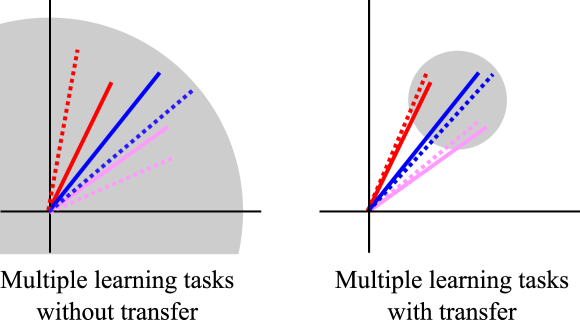
Figure 2: Learning can be viewed as approximating a true concept (solid vectors) with a model (dotted vectors) taken from a class of models (grey ball). Left, three learning tasks (in red, blue & pink) are typically performed independently. Task data is not pooled, and a large class of models may be consistent with the observed data. Right, transfer learning jointly learns a model class common to the tasks thereby implicitly sharing task data and effectively reducing the model class complexity.

3.1 Learning Models

We begin to derive our new transfer learning algorithm for ER by expressing the class of models our algorithm will learn over. For reasons made clear below, we design Transfer to learn linear classifiers; however we later compare this approach against state-of-the-art non-linear algorithms, and we note that the techniques described here are general and can be kernelized to produce non-linear analogues.

3.1.1 Linear Classifiers in ER

Specifying an appropriate model allows us to avoid overfitting the training data. However, as the complexity of our model increases so too does the number of training examples—the sample complexity—required to fit all of the available “degrees of freedom” of our model. Hence, we will need to take the amount of available training data and the learning task at hand into consideration when specifying our model.

In ER [28, 25, 35, 17, 9], and many other problems [20, 30], it has been shown that linear models perform exceptionally well for explaining the behavior between feature score vectors $x$ and output labels $y$. The choice of a linear model serves a dual statistical and computational purpose. Linear models can be evaluated very quickly and are also inexpensive to store, requiring only $p+1$ doubles—together making the model ideal for large-scale learning. From a statistical perspective, given enough features, we can accurately model the interactions in our data. Formally, we assume that a given input set of features $x$ and an output label $y$ can be related by

$$y=\operatorname{sign}(\langle w,\,x\rangle+b)\;,$$

where $b$ is a bias term capturing the fact that the model is not exact due to noise. Here $w$ acts as weight vector, placing varying importance on each of the feature scores in $x$. The setting of $w$ results in splitting our feature score space into two half-spaces, since we have two classes. Finally, we will take our similarity scoring function for a given source pair $(i,j)$ to be

$$f_{ij}(x)=\langle w_{ij},\,x\rangle.$$

Hence the Multi-Source Similarity Learning Problem corresponds to inferring the weight vectors $w_{ij}$.

We will compare the transfer learning approach based on linear models of this section, with both linear and non-linear state-of-the-art baselines in Sections 4 and 5. There is a trade-off: on the one hand, more features allow us to model more interactions, on the other hand, more features result in a more complex model that can be susceptible to overfitting, at a detriment to sample complexity i.e., labeling cost.

3.1.2 Transfer Learning Model

While we have a number of separate tasks across different pairs of sources—naively leading to a quadratic scaling of the sample complexity with the number of sources $r$—one training example from source pair $(i,j)$ could inform learning to score another source pair $(j,h)$ and conceivably even $(h,k)$. This intuition motivates our interest in applying transfer learning to uncover shared characteristics between the different source pair tasks. As borne out in our experiments, doing so will effectively allow us to share examples across many different source pairs in order to most efficiently use the available resources and successfully scale to resolving multiple heterogeneous data sources.

Two extreme forms of transfer are in common use in practice today: either learn each classifier $f_{ij}$ separately (so as to model heterogeneities in the sources at a great labeling cost), or pooling all available data and learning a single classifier (mitigating the labeling cost at the expense of flexibility). Both existing approaches represent two extreme forms of transfer (none and complete transfer, respectively). An ideal method should behave between both extremes and allow the data to dictate the most appropriate behavior. When there is very limited data, we may not have enough information to describe the difference in characteristics between sources. As we gain more information, our method should adapt and take into account any added information. To that end, we introduce a method that we call transfer. For this model, we assume that our weight vectors decompose as

$$w_{ij} = w_{0}+w_{i}+\Delta_{ij}\;,$$ (1)

where the vector $w_{0}$ captures the general trends, for example, movies with the same casts are generally going to be similar. The weight vector $w_{i}$ accounts for the specific effects induced by the particular source and the vector $\Delta_{ij}$ handles the pairwise deviations and can also be applied to guarantee that $w_{ij}=w_{ji}$.

3.2 Regularized Learning Formulation

We now formulate an optimization program for learning the underlying pairwise score functions. There has been a flurry of research in developing efficient techniques for finding parameters that can accurately describe the data using models as those described above. A number of techniques are based on optimizing a convex function for efficiently recovering the parameters. Such convex programs have seen tremendous theoretical and experimental success in the literature [7, 34, 21].

Before proceeding, we recall that the sources are indexed by an integer in $\{1,\ldots,r\}$ so that (abusing notation) $S\in\{1,\ldots,r\}$. Furthermore, we will let $(i(k),j(k))$ denote the source pair that the $k^{th}$ example was drawn from. Given that, we write our $k^{th}$ training example as $(x_{k},S_{1,k},S_{2,k},y_{k})$, where $x_{k}=g(e_{1,k},e_{2,k})$ denotes the feature vector representation of the pair of entities $(e_{1,k},e_{2,k})$, $S_{1,k}$ and $S_{2,k}$ represent the source indices of the entities, and $y_{k}$ represents the true label. With this notation, we may propose to learn an Equation (1) model that solves the convex program

$$\operatorname{argmin}_{w_{0},w_{i},\Delta_{ij}}\underbrace{\frac{1}{2}\sum_{k=1}^{n}(y_{k}-\langle w_{0}+w_{i(k)}+\Delta_{i(k)j(k)},\,x_{k}\rangle)^{2}}_{\text{empirical risk term}}\\ \ \ +\,\underbrace{\lambda\sum_{i=1}^{r}\|w_{i}\|_{1}+\frac{\mu}{2}\sum_{i,j}\|\Delta_{ij}\|_{2}^{2}}_{\text{regularization terms}}\\ \text{s.t. $w_{0}+w_{i}+\Delta_{ij}=w_{0}+w_{j}+\Delta_{ji}$}$$ (2)

The result of this program are estimates of our weight vectors $w_{0}$, $w_{i}$, and $\Delta_{ij}$. We now take a moment to discuss Program (2). The objective function can be decoupled into two components: an empirical risk or loss term and a regularization term.

Loss Term. The loss term aims to encourage predictions on the training input feature vectors to match the training labels. Furthermore, we note that our assumption on the form of the pairwise score functions is built into the optimization procedure. That is, $\langle w_{0}+w_{i}+\Delta_{ij},\,x_{k}\rangle$ should be close to $y_{k}$. We note that there are other alternative options for the loss term such as those used in the logistic regression or support vector machine linear models, both of which are also used extensively in the literature.

Regularization Terms. While the empirical loss term encourages our parameters to closely fit the model, the regularization terms exist in order to penalize overly-complex models and avoid overfitting. For the regularization we penalize the source weight vectors $w_{i}$ by the $\ell_{1}$ norm and the pairwise weight vectors $\Delta_{ij}$ by the $\ell_{2}$ norm squared. These choices have both been extensively studied in the literature due to a number of desirable consequences that they each have. It has been shown that the $\ell_{1}$ norm encourages solutions to convex optimization procedures to be sparse (the $\ell_{1}$ norm essentially acts as a convex surrogate to the $\ell_{0}$ norm, or the total number of non-zero parameters in a vector). Authors have established both theoretical results and experimental results demonstrating the performance of the $\ell_{1}$ norm [33, 7, 11]. By encouraging the $w_{i}$ to be sparse, we capture the fact that each source (for the most part) should behave as the nominal source represented by $w_{0}$. This type of assumption has also appeared in the context of robust regression [15] and low-rank sparse matrix decompositions [8]. The $\ell_{2}$ norm squared terms acts to restrict the size of $\Delta_{ij}$ (without necessarily requiring sparsity), allowing pairwise perturbations away from the nominal behavior between two sources but avoiding overfitting [27]. This choice also accounts for the fact that in general $w_{0}+w_{i}$ will not in general equal $w_{0}+w_{j}$.

Parameter Selection. We may tune the parameters $\lambda$ and $\mu$ to achieve various levels of model complexity and control the amount of transfer. These parameters can be selected via extending existing theoretical results in the literature [3] or based on a user’s prior knowledge for the problem. Another popular method (adopted in this paper) is to apply cross validation, and use a hold-out set of the data to select the parameters [12].

Extending the Learning Algorithm. Our construction allows for a number of choices for the empirical risk and regularization functionals, and we found that our current choices worked well practically from a statistical perspective as well as a computational one. It would be a relatively trivial task to modify our optimization to be more like a pairwise transfer learning version of other linear model-based learners such as logistic regression or SVMs. Our contribution is a generic transfer learning approach for ER which encompasses a family of algorithms; one of which we focus on here as a first study on using transfer in multiple-source ER.

3.3 The Algorithm

We now proceed to derive methods for solving Program (2).

3.3.1 Optimality Conditions

The following result derives from applying the Karush-Kuhn-Tucker (KKT) conditions that govern the program’s optimality conditions [6].

Lemma 2

Suppose that we are given optimal solutions to the convex Program (2): $w^{\star}_{0}$, $w^{\star}_{i}$, and $\Delta^{\star}_{ij}$, and that we let

$$X^{ij} := \sum_{\{k|i(k)=i,j(k)=j\}}x_{k}x_{k}^{T}\;,\quad\text{and}$$

$$g^{ij} := \sum_{\{k|i(k)=i,j(k)=j\}}x_{k}y_{k}\;.$$

Then an application of the KKT conditions yields that

$$\Delta^{\star}_{ij}\;=(X+2\mu I)^{-1}(g-Xw^{\star}_{0}+\mu w^{\star}_{j}-(X+\mu I)w^{\star}_{i})\;.$$

We would like $\Delta^{\star}_{ij}$ to be as small as possible, which would equate to setting $\mu$ as large as possible. Therefore, letting $\mu$ go to $\infty$, we have that

$$\Delta^{\star}_{ij}\;=\frac{1}{2}\left(w^{\star}_{j}-w^{\star}_{i}\right).$$

Therefore, we observe that under $\mu\to\infty$, each $\Delta^{\star}_{ij}$ is simply half the difference between the source vectors $w^{\star}_{i}$ and $w^{\star}_{j}$. Thus, we immediately obtain

$$w^{\star}_{0}+w^{\star}_{i}+\Delta^{\star}_{ij}\;=\;w^{\star}_{0}+\frac{1}{2}\left(w^{\star}_{i}+w^{\star}_{j}\right).$$

The above setting of $\mu$ and subsequent choice of $\Delta^{\star}_{ij}$ is used throughout the remainder of the paper. This model is one that lends itself to far simpler computation since we are only required to compute $w_{i}$ for $0\leq i\leq r$. Furthermore, the model still captures interesting characteristics of each of the sources while learning the common characteristics shared across all sources.

We now present our method for solving Program (2). Standard convex solvers can be employed in the setting when the number of sources and the dimensionality of the problem are small. However, as the number of sources $r$ and the number of dimensions $p$ both grow, we must rely on specialized methods that can overcome the potential computational challenges for solving such minimization programs. Before proceeding we define the loss function to be

$$\mathcal{L}(w^{\star}_{0},w^{\star}_{i})\;=\;\frac{1}{2}\sum_{k=1}^{n}(y_{k}-\langle w_{0}+\frac{1}{2}(w_{i(k)}+w_{j(k)}),\,x_{k}\rangle)^{2}$$

and the regularization terms to be

$$\mathcal{R}(w_{i})\;=\;\lambda\sum_{i=1}^{r}\|w_{i}\|_{1}$$

3.3.2 Solution via Composite Gradient Methods

We now develop a simple algorithm for solving our above convex program based on composite gradient descent methods for optimizing composite objective minimization problems [24]. The method is an iterative algorithm that updates the estimates at each time step based on the current gradients. If we take $w_{i}(s)$ to be the iterate at the $s^{th}$ iteration of the algorithm, then we have that

$$w_{0}(s+1) := w_{0}(s)-\alpha\nabla_{w_{0}}\mathcal{L}(w_{0}(s),w_{i}(s))$$

$$w_{i}(s+1) := S_{\alpha\lambda}\left(w_{i}(s)-\alpha\nabla_{w_{i}}\mathcal{L}(w_{0}(s),w_{i}(s))\right),$$

where $S_{\tau}\left(v\right)$ is the soft-thresholding operator defined on vector $v$, with parameter $\tau$, as

$$S_{\tau}\left(v\right)=\operatorname{sign}(v)\max(|v|-\tau,0)\enspace.$$

Here $\max(|v|-\tau,0)$ is the vector of the same dimension as $v$ whose $i^{th}$ entry is the maximum of $|v_{i}|-\tau$ and zero.

Intuitively, we update the vectors in the direction that will decrease the loss the most. In the case of $w_{i}$, we must also account for the $\ell_{1}$ regularization terms, which result in truncation operations after taking the gradient step. The addition of an $\ell_{1}$ regularization term makes the optimization procedure non-smooth. While we could employ second-order methods [6] for solving this problem, those would be intractable for problems in higher dimensions. Hence, we rely on first-order gradient-based methods for computational tractability. The down-side of applying a gradient-based method is that optimizing general non-smooth functions can become prohibitively slow. However, it has recently been shown that optimizing based on composite objective methods will result in iterates that converge geometrically fast [1].

4 Experiments

We next discuss experiments for verifying the behavior of our transfer learning algorithm and to compare it against the state-of-the-art. The results presented in Section 5 demonstrate significant gains on real-world movie matching and synthetic datasets, showing that Transfer can achieve strong performance with low labeling cost that scales only linear with the number of sources.

4.1 Baseline Approaches

We consider three approaches representing the spectrum of state-of-the-art in ER: pairwise and pooled linear classifiers (which as we argue are actually special cases of transfer learning), and support vector machines (a non-linear learner popular in ER).

Single. The first model, called the Single or Pooled method, simply assumes that $w_{ij}=w_{0}$ for all pairs of sources $i,j$ i.e., by constraining all the $w_{i}=\Delta_{ij}=0$ in Transfer. We have pooled all of the tasks into a single base task—we essentially impose maximum transfer between each task. In this setting, we are effectively required to only estimate $p+1$ parameters, which can be done very effectively with order $p$ training examples [23]. Hence, we have greatly reduced the model complexity of the problem at the expensive of ignoring any of the unique behavior of individual sources.

Pairwise Independent. At the other extreme, the method PairwiseIndependent considers the situation where all normal vectors $w_{ij}$ are learned without any shared characteristics. This setting has no transfer as we make no assumption as to the structure between the tasks of learning pairwise scoring functions. The model complexity is prohibitively large since the number of parameters to estimate scales as $r^{2}p$. Hence, we would require order $r^{2}p$ training examples just to learn each of the classifiers. However under heterogeneous sources, with enough data, this approach should achieve far superior accuracy over Single.

Non-linear. Our third baseline model, denoted NonLinear, involves learning a non-linear function. Unlike the above linear models that take a weighted sum of the pairwise attributes, the non-linear learner will return an arbitrary function on the features. So that NonLinear may vary its output depending on the originating sources, it is natural to encode the source pair identities in addition to the feature scores—the feature vector presented is $(g(e_{i}),g(e_{j}),i,j)$ with source pair $(i,j)$ encoded into a length $r$ vector that is all zeros except a $1$ in the $i^{th}$ and $j^{th}$ components (since source ordering is irrelevant). In this way NonLinear has the flexibility of modeling sources individually, while implicitly transferring patterns learned between sources. For our experiments we take NonLinear to be the support vector machine (SVM) with Gaussian kernel, which corresponds to the most widely used and flexible feature mapping. This SVM takes in two parameters: the cost parameter $C>0$ and the kernel variance $\sigma>0$.

Remark 3

Single and PairwiseIndependent are both special (extreme) cases of Transfer and are also of independent interest since together they represent one kind of state-of-the-art technique—linear classification—that has enjoyed success in ER [28, 25, 35, 17, 9]. With adaptively selected parameters (via cross validation), we expect Transfer to find a balance between the label-economical but inflexible Single and the flexible but label-hungry PairwiseIndependent.

SVMs are regarded as one of the most effective learners in ER [19, 18, 4, 26, 10, 5, 22, 17]. Like Transfer, the SVM can adapt its model complexity for the problem (via its parameters). However to take advantage of its flexibility over linear methods more data is typically needed. Moreover while it may learn different classifications for different sources (as these are encoded in the feature vector), and indeed transfer between these tasks, the SVM does not possess the pairwise structural knowledge that is built in to Transfer.

4.2 Algorithm Implementation

For our experiments, we implement Transfer as described in Section 3 in the statistical computing environment R. We implement the baseline Single and PairwiseIndependent algorithms based off of the more general Transfer implementation; however to speed up the baseline algorithms in-line with fast state-of-the-art implementations—for fair and representative comparisons in our timing experiments—we exploit standard computational tricks not available for the general transfer learning case.

We use the R e1071 package’s SVM routines, which are a wrapper for the popular libSVM library, for implementing NonLinear. We employ 10-fold cross-validation for selecting optimal SVM parameters $(C,\sigma)$ over a grid of candidates as is standard.

4.3 Evaluation

IMDB	AMG	Flixster	MSN	Netflix	iTunes
526k	306k	141k	104k	76k	12.5k

Table 1: The number of entities per crawled movie data source.

In order to investigate the statistical performance of the methods’ scores, we adopt a common threshold algorithm: we declare that two entities $e_{1}$ and $e_{2}$ are a match if their score is above threshold $\tau$, which we vary to produce a set of potential classifiers. Therefore, given a scoring function $f$ and a set of examples $\{(x_{k},y_{k})\}$, we aim to compare the true labels $y_{k}$ against the estimated labels

$$\widehat{y}_{k}=\operatorname{sign}(f(x_{k})-\tau)\enspace.$$

We evaluate the performance of classifier’s classifications through precision and recall, defined in the usual way as follows.

Definition 4

Let

$$TP :=\{k|\widehat{y}_{k}=y_{k}=1\}\quad\text{be the set of true positives,}$$

$$FP :=\{k|\widehat{y}_{k}=1\;\text{and}\;y_{k}=0\}\quad\text{be the set of false positives,}$$

$$FN :=\{k|\widehat{y}_{k}=0\;\text{and}\;y_{k}=1\}\quad\text{be the set of false negatives.}$$

We define precision $P$ and recall $R$ in terms of these sets:

$$P:=\frac{|TP|}{|TP|+|FP|} R:=\frac{|TP|}{|TP|+|FN|}.$$

Hence, for varying threshold $\tau$, we have a range of different $P$ and $R$ values that together to form a precision-recall curve. We also measure test error as follows, which combines both false positives and negatives.

$$E:=\frac{1}{m}\sum_{k}\mathbb{I\,}(y_{k}\neq\widehat{y}_{k}).$$ (3)

4.4 Datasets and Pre-Processing

We employed two large-scale datasets in our experiments.

Real-World Move Data. Six major online movie sources were crawled for use in the Bing movies vertical. The number of records obtained are given in Table 1. For each movie we obtained its title and alternate titles, release year, runtime, cast, and directors. From these attributes we performed basic string cleanup and blocked on common (non-stop) words in the titles. Each raw feature produced one feature score: Jaccard for titles, directors and cast; and absolute difference for runtime and year. Humans labeled 200 entity pairs across each source pair. In our following experimental results on this movie data, we learn the scoring functions on various sources (as specified) but evaluate precision and recall against movies from the pair IMDB and iTunes. This choice was made in order to demonstrate the behavior across a specific pair rather than averaging across all available pairs. We held out a subset of the movie data as the test set. We then used the remainder for training the methods. In order to improve the conditioning of the problem, as is standard in machine learning, we standardized the data by subtracting feature score means and dividing by standard deviation, making the features zero mean and unit variance and so placing the features on equal footing.

Synthetic Data. We synthesized raw true attributes for each underlying latent entity uniformly at random in a unit interval. Then each record representing an entity in a source was produced by perturbing each of the attributes randomly with low-variance Gaussian noise. Feature-level scores were then produced using a simple difference between the attribute values of pairs of entities. It is important to note that perturbing the feature-level scores would be an incorrect methodology since the scores would not observe any kind of triangle-inequality-like property as is the case for “real” ER problems. We produced up to 30 synthetic sources to stress test the approaches, and used 10k test pairs total.

Figure 3: Precision achieved by each method on the 6 movie sources, at 0.85 recall, for varying number of examples.

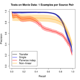
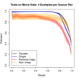
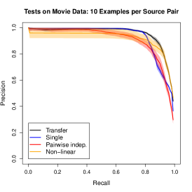
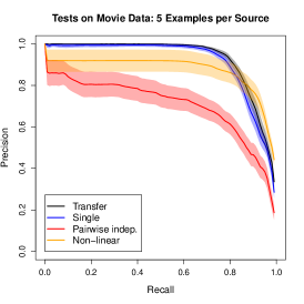
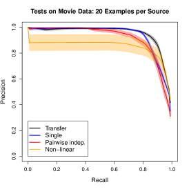
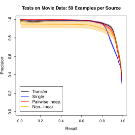
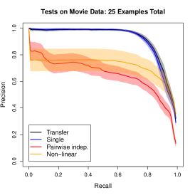
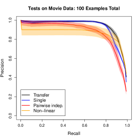
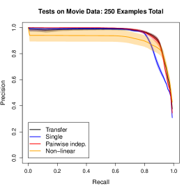
Figure 4: Precision-recall curves comparing the four learning algorithms on the 6 sources of movie matching data; bands show 95% pointwise confidence intervals. Figures in the top/middle/bottom row show methods trained on numbers of examples per source pair/source/total; and figures in columns see increasing training data going from left to right.

Figure 5: Sample complexity of the three linear learning algorithms on synthetic data.

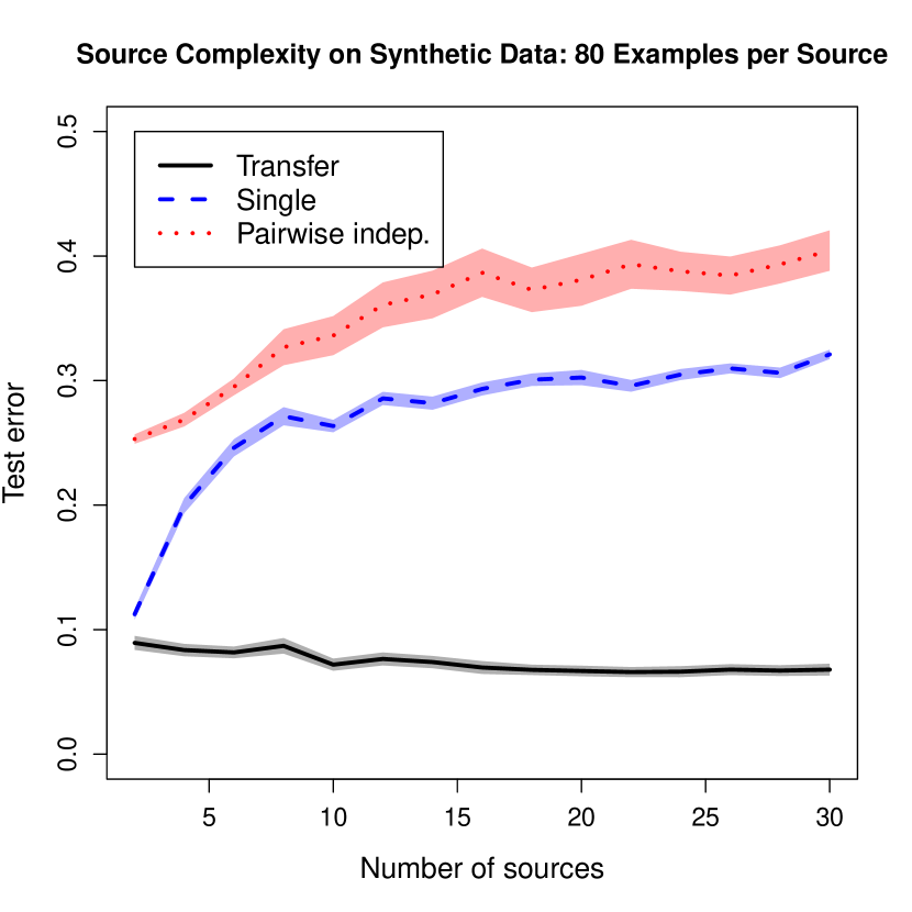
Figure 6: Source complexity of the three linear learning algorithms on synthetic data.

5 Results

We now present the results of our experiments, starting on the movie data. These results are presented by comparing the PR curves of Transfer and the three baseline methods. We then focus attention on the synthetic data in order to gain a deeper understanding of the behavior of the transfer method. Our results conclusively demonstrate that Transfer requires significantly less labeling while achieving superior accuracy over state-of-the-art approaches in multiple-source ER.

5.1 Precision Recall Curves

With the datasets selected, we applied the four learning algorithm to the training set, producing pairwise functions $f_{ij}$. We then applied the functions to the unobserved test data and built PR curves by varying threshold parameter $\tau$. Figure 4 presents a three by three grid of PR curves. These figures each represent the effects of varying the number of training examples on the precision and recall. Figure 3 summarizes these nine plots by fixing recall at 0.85—matching for a movie vertical requires high precision at the expense of lower recall—and visualizing achieved precision against total number of training examples.

Consider the summary Figure 3. As expected Single performs relatively well when very little training data is available, but does not experience much gain from additional training data—and is inferior to the other methods—owing to it not modeling the unique data characteristics of each source. PairwiseIndependent behaves in the opposite manner to Single: it just not able to fit its many-parameter models under little available data, but progressively improves as more data becomes. Transfer combines the best of both of the linear baseline models adaptively, and dominates all three state-of-the-art baselines at 0.85 recall. While NonLinear traces the performance of Transfer, it is not endowed with the correct pairwise task structure leveraged by Transfer and so its precision is significantly shifted down.

Similar patterns are born out in the complete PR curves of Figure 4 which are also endowed with 95% confidence bands. In its first, second and third rows we vary the number of available examples per source pair, per source, and in total, respectively. The same trends observed in Figure 3 are apparent here, however one method does not tend to dominate another for all recall values.

In the final row and column, PairwiseIndependent catches up with Transfer, because the two sources that were picked to construct the PR curves are themselves large, so that a large number of training examples were assigned to that specific pair. Another interesting observation is that NonLinear varies significantly compared to the other methods (apparent from the width of the confidence bands). Such behavior is to be expected as the model complexity for NonLinear is the greater. Due to its poor performance on the movie data, we do not present results for NonLinear SVM on the synthetic data, where we focus on an apples-to-apples comparison of the three linear learners with varying amounts of transfer.

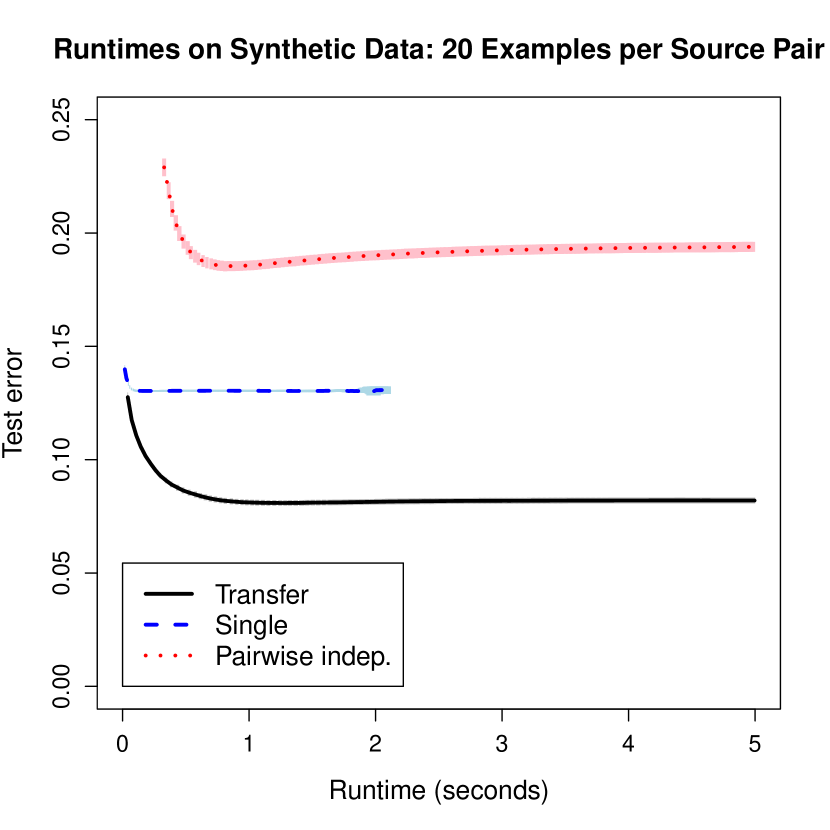
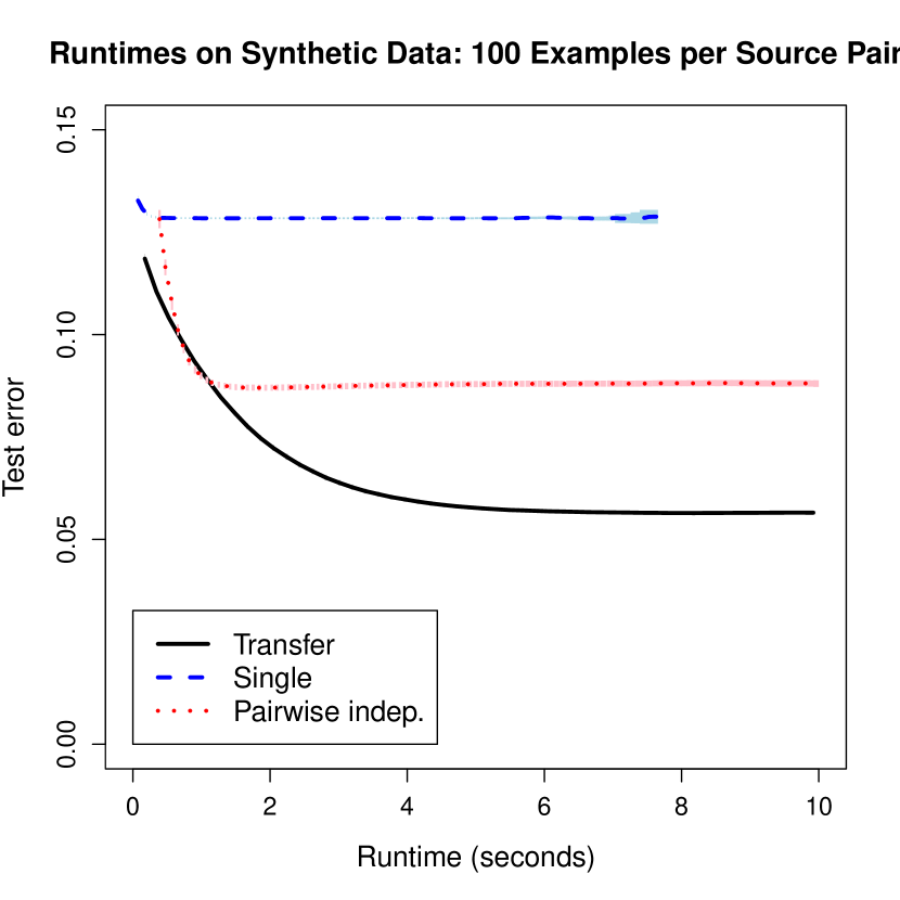
Figure 7: Runtime analysis of the three learning algorithms on (left) 20 (right) 100 examples per synthetic source pair. Across the board transfer yields superior performance after only a short time. Pairwise independent surpasses pooled once it is given around 40 examples per source pair.

5.2 Sample Complexity

Our next experiment takes a deeper look at understanding the effect of the number of examples per source pair on the average error defined in Equation (3). These experiments were performed using synthetic data to give us finer control over the data generating process and thus concretely explore how increasing the number of examples will affect $E$. We observe from Figure 5, that as the number of examples increases Transfer and PairwiseIndependent both decrease, while Single remains lower bounded. This result is owing to the fact that Single cannot take into account the individual differences between the sources that we are experimenting with, while the other more flexible methods can. However, even though PairwiseIndependent does have that freedom, we see that Transfer still performs better because it is a “simpler” model to learn.

5.3 Source Complexity

We now present results of one of our most poignant synthetic experiments. Figure 6 shows the results of increasing the number of synthetic sources from 2 to 30 in increments of 2 sources. As we increase the number of sources we add a constant number of training examples—we impose desirable linear not intractable quadratic labeling cost scaling. Again we compare the three linear methods, along with their confidence bands based on 50 trials. We observe that Transfer achieves far-superior results, actually improving slightly with the number of sources. On the other hand, we see that PairwiseIndependent, unsurprisingly, performs poorly as the number of sources increase as it requires quadratic scaling of the training data. The algorithm no longer has sufficient available examples to train the order of 450 scoring functions. We also note that even though Single is very “simple”, and hence does not require a significant amount of training examples, it is unable to adapt to the fact that the sources have varying behavior. Hence, we observe the error increase as the Single method is no longer able to model the behavior of the observed examples.

5.4 Runtime Analysis

Figure 7 shows the results of a timing analysis of the three linear methods. In the left figure we show the results with 20 examples per source pair, and in the right we show 100 examples per source pair, both on 10 synthetic sources. In both cases Transfer quickly achieves superior test error and converges relatively fast. The baseline linear methods converge faster but to inferior test error. In the small training set case Single outperforms PairwiseIndependent, and as expected as the number of training examples increases to 100 examples per source pair, PairwiseIndependent overtakes Single and performs comparably to Transfer.

6 Related Work

We now discuss prior work in ER as it is related to this paper, from the viewpoints of ER across sources of varying quality, and recognizing (and mitigating) the cost of generating labeled data. This paper is one of the first to consider ER on multiple sources of varying quality, is the first to highlight cost of labeling as a barrier to scaling accurate ER to multiple sources, and is the first to apply the transfer learning paradigm to ER (and along the way we develop a transfer learning algorithm that is novel to the machine learning community).

Varying Source Quality. Numerous works have studied ER, many of which involving matching across multiple sources, but very few have explored the serious challenge of resolving sources with varying data quality. Traditionally researchers use a single non-learning-based matcher or model a single learner on pooled training data [29]. Shen et al.posited that real-world data sources have varying levels of semantic ambiguity, a special case of source quality in which an individual attribute should be given more or less weight. They propose the SOCCER framework for compiling matching execution plans in which one of two matchers can be employed on different sources—a relaxed (conservative) matcher requiring less (respectively more) evidence to declare a match. These matchers could be related via the relaxation of a threshold, for example. Similar to [29], the adverse effect of heterogeneous source quality on matching accuracy is a key motivation of this paper. By contrast, however, our paper sets out to learn continuous characterizations of quality via real-valued weights, over all attributes together. Moreover we leverage a significantly more fine-grained transfer structure between the tasks of matching different source pairs, compared to the authors’ process of simply pooling like tasks—which is more akin to the straw man Single learner used for comparison here, which does not correctly balance transfer with the needs of matching tasks.

Köpcke & Rahm developed the STEM framework for investigating the effect of training selection on learning to match [17]. While they do not compare training on heterogeneous sources independently in a pairwise fashion versus together with a single matcher, they implicitly acknowledge the need to produce different matchers tailored to source-pairs’ characteristics as they split their most challenging experimental matching task of resolving publications between three sources—Google Scholar (larger but of lower quality), DBLP and the ACM Digital Library (both higher quality but smaller)—into independent learning problems between DBLP and the other two sources.

The Cost of Labeling. The key challenge solved by our approach is to significantly reduce the human effort required to label training data for learning to combine matchers over multiple domains. In their thorough comparative evaluations of 21 ER systems with their FEVER framework [19], Köpcke et al.explicitly identified human effort as a key metric for the effectiveness of learning-based ER systems. In their line of work, this desire can be traced to their earlier paper on STEM [17]. In both works the authors pay particular attention to the effect of training-set size on the quality of matching, and favor methods requiring less labeled data such as the SVM. Unlike this paper, however, they do not consider matching across multiple sources and the additional requirement this can place on human labeling.

While low sample complexity has been identified as a desirable property of entity matchers, the notion of labeling cost has not been previously recognized as a barrier to scaling ER. We introduce the notion of source complexity which characterizes the change in error as new sources are added, provided the number of training examples are increased only linearly with the sources.

7 Conclusions

Many problems in databases, statistics and machine learning require learning of a pairwise similarity function from human-labeled examples. However as the number of data sources increases, the sample complexity—the cost of human labeling—increases quadratically. To overcome this prohibitive scaling, we propose a new transfer learning algorithm Transfer for learning multiple similarity score functions jointly. We take ER as a motivating example, and present extensive experimental comparisons of Transfer against existing state-of-the-art methods. Our experiments—on real-world, large scale movie matching data, and extensive synthetic data—show that Transfer indeed produces more accurate results for ER than existing methods, with less data, and indeed in faster time. Interesting future work might consider combining active learning with Transfer, and extending Transfer to non-linear classification.

8 Acknowledgments

We thank Ashok Chandra, Ariel Fuxman, Duo Zhang and Bo Zhao for their valuable comments and assistance.

References

- [1] A. Agarwal, S. Negahban, and M. J. Wainwright. Fast global convergence rates of gradient methods for high-dimensional statistical recovery. In NIPS’2010, pages 37–45, 2010.
- [2] R. Ando and T. Zhang. A framework for learning predictive structures from multiple tasks and unlabeled data. J. Machine Learning Res., 6:1817–1853, 2005.
- [3] P. J. Bickel, Y. Ritov, and A. Tsybakov. Simultaneous analysis of Lasso and Dantzig selector. Ann. Statistics, 37(4):1705–1732, 2009.
- [4] M. Bilenko and R. J. Mooney. Adaptive duplicate detection using learnable string similarity measures. In KDD’03, 2003.
- [5] M. Bilenko and R. J. Mooney. On evaluation and training-set construction for duplication detection. In Proceedings of the KDD-2003 Workshop on Data Cleaning, Record Linkage, and Object Consolidation, 2003.
- [6] S. Boyd and L. Vandenberghe. Convex Optimization. Cambridge University Press, 2004.
- [7] E. Candes and T. Tao. Decoding by linear programming. IEEE Trans. Info. Theory, 51(12):4203–4215, 2005.
- [8] V. Chandrasekaran, S. Sanghavi, P. A. Parrilo, and A. S. Willsky. Rank-sparsity incoherence for matrix decomposition. SIAM Journal on Optimization, 21(2), June 2011.
- [9] Z. Chen, D. V. Kalashnikov, and S. Mehrotra. Exploiting context analysis for combining multiple entity resolution systems. In SIGMOD’09, pages 207–218, 2009.
- [10] P. Christen. FEBRL: a freely available record linkage system with a graphical user interface. In Proceedings of the Second Australasian Workshop on Health Data and Knowledge Management, pages 17–25, 2008.
- [11] D. L. Donoho. Compressed sensing. IEEE Trans. Info. Theory, 52(4), April 2006.
- [12] B. Efron, T. Hastie, I. Johnstone, and R. Tibshirani. Least angle regression. Annals of Statistics, 32(2):407–499, 2004.
- [13] A. K. Elmagarmid, P. G. Ipeirotis, and V. S. Verykios. Duplicate record detection: A survey. IEEE Trans. Knowledge and Data Eng., 19(1):1–16, 2007.
- [14] J. Huang and T. Zhang. The benefit of group sparsity. Ann. Statistics, 38(4):1978–2004, 2010.
- [15] A. Jalali, P. Ravikumar, S. Sanghavi, and C. Ruan. A dirty model for multi-task learning. In NIPS’2010, 2010.
- [16] C. W. Kelman, M. A. Kortt, N. G. Becker, Z. Li, J. Mathews, C. Guest, and C. Holman. Deep vein thrombosis and air travel: record linkage study. BMJ, 327(7423):1072, 2003.
- [17] H. Köpcke and E. Rahm. Training selection for tuning entity matching. In Proc. Int. Work. Quality in Databases and Manag. of Uncertain Data, pages 3–12, 2008.
- [18] H. Köpcke and E. Rahm. Frameworks for entity matching: A comparison. Data & Knowledge Eng., 69(2):197–210, 2010.
- [19] H. Köpcke, A. Thor, and E. Rahm. Evaluation of entity resolution approaches on real-world match problems. PVLDB, 3(1), 2010.
- [20] J. S. Lawson. Record linkage techniques for improving online genealogical research using census index records. In Proc. Section on Survey Research Methods, pages 3297–3303. American Statistical Assoc., 2006.
- [21] H. Liu, J. Lafferty, and L. Wasserman. Nonparametric regression and classification with joint sparsity constraints. In NIPS’2008, 2008.
- [22] S. Minton, C. Nanjo, C. A. Knoblock, M. Michalowski, and M. Michelson. A heterogeneous field matching method for record linkage. In ICDM’2005, pages 314–321, 2005.
- [23] S. Negahban, P. Ravikumar, M. J. Wainwright, and B. Yu. A unified framework for high-dimensional analysis of -estimators with decomposable regularizers. In NIPS’2009, pages 1348–1356, 2009. Full length version arxiv:1010.2731v1.
- [24] Y. Nesterov. Gradient methods for minimizing composite objective function. Technical Report 76, Center for Operations Research & Econometrics, Catholic University of Louvain, 2007.
- [25] J. C. Pinheiro and D. X. Sun. Methods for linking and mining massive heterogeneous databases. In KDD’98, 1998.
- [26] S. Sarawagi and A. Bhamidipaty. Interactive deduplication using active learning. In KDD’02, pages 269–278, 2002.
- [27] B. Schölkopf and A. J. Smola. Learning with Kernels. MIT Press, 2001.
- [28] A. Segev and A. Chatterjee. A framework for object matching in federated databases and its implementation. Int. J. Cooperative Info. Sys., 5(1):73–99, 1996.
- [29] W. Shen, P. DeRose, L. Vu, A. Doan, and R. Ramakrishnan. Source-aware entity matching: A compositional approach. In ICDE’07, pages 196–205, 2007.
- [30] N. Srebro, J. Rennie, and T. S. Jaakkola. Maximum-margin matrix factorization. In NIPS’04, 2004.
- [31] A. J. Storkey, C. K. I. Williams, E. Taylor, and R. G. Mann. An expectation maximisation algorithm for one-to-many record linkage, illustrated on the problem of matching far infra-red astronomical sources to optical counterparts. Technical report, University of Edinburgh, 2005.
- [32] S. Tejada, C. A. Knoblock, and S. Minton. Learning domain-independent string transformation weights for high accuracy object identification. In KDD’02, 2002.
- [33] R. Tibshirani. Regression shrinkage and selection via the lasso. Journal of the Royal Statistical Society, Series B, 58(1), 1996.
- [34] S. A. van de Geer. High-dimensional generalized linear models and the lasso. Ann. Statistics, 36:614–645, 2008.
- [35] H. Zhao and S. Ram. Entity identification for heterogeneous database integration: a multiple classifier system approach and empirical evaluation. Info. Sys., 30(2):119–132, 2005.