Determinantal Quintics and Mirror Symmetry of Reye Congruences

Abstract.

We study a certain family of determinantal quintic hypersurfaces in $\mathbb{P}^{4}$ whose singularities are similar to the well-studied Barth-Nieto quintic. Smooth Calabi-Yau threefolds with Hodge numbers $(h^{1,1},h^{2,1})=(52,2)$ are obtained by taking crepant resolutions of the singularities. It turns out that these smooth Calabi-Yau threefolds are in a two dimensional mirror family to the complete intersection Calabi-Yau threefolds in $\mathbb{P}^{4}\times\mathbb{P}^{4}$ which have appeared in our previous study of Reye congruences in dimension three. We compactify the two dimensional family over $\mathbb{P}^{2}$ and reproduce the mirror family to the Reye congruences. We also determine the monodromy of the family over $\mathbb{P}^{2}$ completely. Our calculation shows an example of the orbifold mirror construction with a trivial orbifold group.

1. Introduction

Quintic hypersurfaces in the projective space $\mathbb{P}^{4}$ have been invaluable testing grounds for the interesting mathematical ideas coming from the string theory. This has been for long since the historical discovery of an exact solution of N=2 superconformal field theory/string theory and its profound relations to the quintic hypersurfaces [Gep]. The idea of mirror symmetry of Calabi-Yau manifolds, for example, has been verified first by translating a special involution in the set of N=2 theories into some operation, now-called orbifold mirror construction, in the algebraic geometry of quintic hypersurfaces [GP], [Yau], and also the surprising applications of the mirror symmetry to Gromov-Witten theory have been started from the Hodge theoretical investigations of the mirror quintic hypersurfaces [CdOGP].

In this paper, we will be concerned with certain special types of quintic hypersurfaces in $\mathbb{P}^{4}$ which are called determinantal quintics. The determinantal quintics are interesting not only from the viewpoint of the mirror symmetry but also from the viewpoint of the classical projective geometry. In fact these quintics have appeared in our previous study of the so-called Reye congruences in dimension three [HT], where a beautiful interplay between the mirror symmetry and the classical projective geometry has been observed. Historically, Reye congruences represent certain Enriques surfaces, called nodal Enriques surfaces [Co], [Ty], and their study goes back to the 19th century, where the term ‘congruence‘ arose in relation to the geometry of the Grassmannian $G(2,4)$. They naturally come with K3 surfaces which admit fixed point free involutions. In dimension three, the corresponding Reye congruences turn out to be Calabi-Yau manifolds with non-trivial fundamental groups [Ol], and they also come with Calabi-Yau threefolds equipped with fixed point free involutions which we call covering Calabi-Yau threefolds of the Reye congruences.

In our previous work [HT], we have studied the mirror symmetry of the three dimensional Reye congruences through the covering Calabi-Yau threefolds using the methods in the toric geometry [BaBo]. In this paper, we will reconsider the mirror symmetry based on the orbifold mirror construction and will observe that the projective geometries of certain singular determinantal quintics come into play in an interesting way. Also we find that, in our case, the so-called orbifold group is a trivial group, $G_{orb}=\{{\rm id}\}$. The last property naturally leads us to a problem that how is the mirror involution in the corresponding N=2 string theory realized in such cases, although we will not discuss the problem in this article.

The construction of this paper is as follows: In the next section we will summarize the geometries of the Reye congruences following the previous work. There, after setting up the notation and the problems in details, we describe the main results of this paper. In Section 3, we calculate the topological Euler numbers of certain (singular) determinantal quintic hypersurfaces. In Section 4, we describe the details about the calculations of some Euler numbers needed in Section 3. In Section 5, we will obtain the mirror family to the covering Calabi-Yau threefolds of the Reye congruences. In Section 6, we will determine completely the monodromy properties of the mirror family. Taking the fixed point free involution into account, we construct the mirror family to the Reye congruences. In Section 7, we will discuss some geometry of the singular Hessian quintics.

Acknowledgements: The authors would like to thank Prof. B. van Geemen for his kind and helpful correspondence to their question about the étale cohomology. They also would like to thank Prof. C. Vafa for his correspondence. This work is supported in part by Grant-in Aid Scientific Research (C 22540041, S.H.) and Grant-in Aid for Young Scientists (B 30322150, H.T.).

2. Backgrounds and summary of main results

2.1. Three dimensional Reye congruences

Let us consider the product $\mathbb{P}^{4}\times\mathbb{P}^{4}$ of the complex projective spaces with its bi-homogeneous coordinate $([z],[w])$. We consider a generic complete intersection $\tilde{X}_{0}$ of five $(1,1)$ divisors in the product. In terms of the bi-homogeneous coordinates, $\tilde{X}_{0}$ may be written by $f_{1}=\cdots=f_{5}=0$ in $\mathbb{P}^{4}\times\mathbb{P}^{4}$, where we set $f_{k}:=\,^{t}zA_{k}w$ with $5\times 5$ matrices $A_{1},...,A_{5}$ over $\mathbb{C}$. When $A_{k}$ are generic, $\tilde{X}_{0}$ defines a smooth Calabi-Yau threefold with its Hodge numbers $h^{11}(\tilde{X}_{0})=2,h^{21}(\tilde{X}_{0})=52$. Despite this simple descriptions, $\tilde{X}_{0}$ has interesting birational geometries which we summarize in the following diagram:

(2.1) $$\begin{matrix}\lx@xy@svg{\hbox{\raise 0.0pt\hbox{\kern 7.17778pt\hbox{\ignorespaces\ignorespaces\ignorespaces\hbox{\vtop{\kern 0.0pt\offinterlineskip\halign{\entry@#!@&&\entry@@#!@\cr&&\\&&&\crcr}}}\ignorespaces{\hbox{\kern-7.17778pt\raise 0.0pt\hbox{\hbox{\kern 0.0pt\raise 0.0pt\hbox{\hbox{\kern 3.0pt\raise 0.0pt\hbox{$\textstyle{\tilde{X}_{0}\ignorespaces\ignorespaces\ignorespaces\ignorespaces}$}}}}}}}\ignorespaces\ignorespaces\ignorespaces{}\ignorespaces\ignorespaces{\hbox{\lx@xy@drawline@}}\ignorespaces\ignorespaces\ignorespaces{\hbox{\kern 19.6743pt\raise-14.97362pt\hbox{{}\hbox{\kern 0.0pt\raise 0.0pt\hbox{\hbox{\kern 3.0pt\hbox{\hbox{\kern 0.0pt\raise-0.8625pt\hbox{$\scriptstyle{\pi_{2}}$}}}\kern 3.0pt}}}}}}\ignorespaces{\hbox{\kern 31.17778pt\raise-31.75444pt\hbox{\hbox{\kern 0.0pt\raise 0.0pt\hbox{\lx@xy@tip{1}\lx@xy@tip{-1}}}}}}\ignorespaces\ignorespaces{\hbox{\lx@xy@drawline@}}\ignorespaces{\hbox{\lx@xy@drawline@}}{\hbox{\kern 36.34862pt\raise 0.0pt\hbox{\hbox{\kern 0.0pt\raise 0.0pt\hbox{\hbox{\kern 3.0pt\raise 0.0pt\hbox{$\textstyle{}$}}}}}}}{\hbox{\kern 71.51945pt\raise 0.0pt\hbox{\hbox{\kern 0.0pt\raise 0.0pt\hbox{\hbox{\kern 3.0pt\raise 0.0pt\hbox{$\textstyle{\ignorespaces\ignorespaces\ignorespaces\ignorespaces\tilde{X}_{2}\ignorespaces\ignorespaces\ignorespaces\ignorespaces}$}}}}}}}\ignorespaces\ignorespaces\ignorespaces{}\ignorespaces\ignorespaces{\hbox{\lx@xy@drawline@}}\ignorespaces\ignorespaces\ignorespaces{\hbox{\kern 47.50105pt\raise-14.93813pt\hbox{{}\hbox{\kern 0.0pt\raise 0.0pt\hbox{\hbox{\kern 3.0pt\hbox{\hbox{\kern 0.0pt\raise-0.8264pt\hbox{$\scriptstyle{p_{1}}$}}}\kern 3.0pt}}}}}}\ignorespaces{\hbox{\kern 47.51945pt\raise-31.74646pt\hbox{\hbox{\kern 0.0pt\raise 0.0pt\hbox{\lx@xy@tip{1}\lx@xy@tip{-1}}}}}}\ignorespaces\ignorespaces{\hbox{\lx@xy@drawline@}}\ignorespaces{\hbox{\lx@xy@drawline@}}\ignorespaces\ignorespaces\ignorespaces{}\ignorespaces\ignorespaces{\hbox{\lx@xy@drawline@}}\ignorespaces\ignorespaces\ignorespaces{\hbox{\kern 99.11761pt\raise-14.84694pt\hbox{{}\hbox{\kern 0.0pt\raise 0.0pt\hbox{\hbox{\kern 3.0pt\hbox{\hbox{\kern 0.0pt\raise-0.8264pt\hbox{$\scriptstyle{p_{2}}$}}}\kern 3.0pt}}}}}}\ignorespaces{\hbox{\kern 109.87502pt\raise-30.37587pt\hbox{\hbox{\kern 0.0pt\raise 0.0pt\hbox{\lx@xy@tip{1}\lx@xy@tip{-1}}}}}}\ignorespaces\ignorespaces{\hbox{\lx@xy@drawline@}}\ignorespaces{\hbox{\lx@xy@drawline@}}{\hbox{\kern-3.0pt\raise-40.0689pt\hbox{\hbox{\kern 0.0pt\raise 0.0pt\hbox{\hbox{\kern 3.0pt\raise 0.0pt\hbox{$\textstyle{}$}}}}}}}{\hbox{\kern 31.17778pt\raise-40.0689pt\hbox{\hbox{\kern 0.0pt\raise 0.0pt\hbox{\hbox{\kern 3.0pt\raise 0.0pt\hbox{$\textstyle{Z_{2}}$}}}}}}}{\hbox{\kern 75.69724pt\raise-40.0689pt\hbox{\hbox{\kern 0.0pt\raise 0.0pt\hbox{\hbox{\kern 3.0pt\raise 0.0pt\hbox{$\textstyle{}$}}}}}}}{\hbox{\kern 109.87502pt\raise-40.0689pt\hbox{\hbox{\kern 0.0pt\raise 0.0pt\hbox{\hbox{\kern 3.0pt\raise 0.0pt\hbox{$\textstyle{\tilde{X}_{0}^{\sharp}\;,}$}}}}}}}\ignorespaces}}}}\ignorespaces\end{matrix} \textstyle{\tilde{X}_{0}\ignorespaces\ignorespaces\ignorespaces\ignorespaces} \scriptstyle{\pi_{2}} \textstyle{\ignorespaces\ignorespaces\ignorespaces\ignorespaces\tilde{X}_{2}\ignorespaces\ignorespaces\ignorespaces\ignorespaces} \scriptstyle{p_{1}} \scriptstyle{p_{2}} \textstyle{Z_{2}} \textstyle{\tilde{X}_{0}^{\sharp}\;,} \textstyle{\tilde{X}_{0}\ignorespaces\ignorespaces\ignorespaces\ignorespaces} \scriptstyle{\pi_{2}} \textstyle{\ignorespaces\ignorespaces\ignorespaces\ignorespaces\tilde{X}_{2}\ignorespaces\ignorespaces\ignorespaces\ignorespaces} \scriptstyle{p_{1}} \scriptstyle{p_{2}} \textstyle{Z_{2}} \textstyle{\tilde{X}_{0}^{\sharp}\;,}$$

where $Z_{2}$ and $\tilde{X}_{0}^{\sharp}$ are determinantal quintics defined by

$$Z_{2}=\left\{\;[w]\in\mathbb{P}^{4}\mid{\rm det}(A_{1}wA_{2}w...A_{5}w)=0\right\},$$

and

$$\tilde{X}_{0}^{\sharp}=\left\{[\lambda]\in\mathbb{P}_{\lambda}^{4}\biggl{|}\text{det}\bigl{(}\sum_{k=1}^{5}\lambda_{k}A_{k}\bigr{)}=0\right\},$$

respectively, and $\tilde{X}_{2}$ is defined by

$$\tilde{X}_{2}=\left\{[w]\times[\lambda]\in\mathbb{P}^{4}\times\mathbb{P}_{\lambda}^{4}|\,A_{\lambda}w=0\right\},\text{ where }A_{\lambda}=\sum_{k=1}^{5}\lambda_{k}A_{k}.$$

$\mathbb{P}_{\lambda}^{4}$ is the projective space defined from the $\mathbb{C}$-vector space spanned by the matrices $A_{k}(k=1,...,5)$. The maps $\pi_{2}$ and $p_{i}\,(i=1,2)$ in the diagram (2.1) are defined by the natural projections; the projection to the second factor $\mathbb{P}^{4}\times\mathbb{P}^{4}\rightarrow\mathbb{P}^{4}$ for $\pi_{2}$, and the projections from $\mathbb{P}^{4}\times\mathbb{P}_{\lambda}^{4}$ to the first and the second factors for $p_{i}\,(i=1,2)$, respectively. As we can see in the definitions, both $Z_{2}$ and $\tilde{X}_{0}^{\sharp}$ are quintic hypersurfaces in the respective projective spaces, and $\tilde{X}_{2}$ is a complete intersection of five $(1,1)$ divisors in the product $\mathbb{P}^{4}\times\mathbb{P}_{\lambda}^{4}$. When the matrices $A_{k}$ are generic, the both $Z_{2}$ and $\tilde{X}_{0}^{\sharp}$ determine generic determinantal varieties in $\mathbb{P}^{4}$ and $\mathbb{P}_{\lambda}^{4}$, respectively. Generic determinantal varieties are known to be singular along codimension three loci, where the matrices have corank two (see [HT, Lemma 3.2] for example). In our case, the degree of the singular loci is 50. Hence generic $Z_{2}$ and $\tilde{X}_{0}^{\sharp}$ are singular at 50 points, where the rank of the relevant matrices decreases to three, and actually these consist of 50 ordinary double points [ibid. Proposition 3.3]. We also note that $\tilde{X}_{0}$ and $\tilde{X}_{2}$ are birational but not isomorphic in general [ibid. Sect.(3-2)].

The geometries of $\tilde{X}_{0}$ and $\tilde{X}_{0}^{\sharp}$ in the above diagram fit well to the classical projective duality, since the projective dual $(\mathbb{P}^{4}\times\mathbb{P}^{4})^{*}$ to the Segre variety $\mathbb{P}^{4}\times\mathbb{P}^{4}\hookrightarrow\mathbb{P}^{24}$ is naturally given by the determinantal variety in the dual projective space $(\mathbb{P}^{24})^{*}$ and $\tilde{X}_{0}^{\sharp}$ is given by a linear section of this determinantal variety. Based on this, in [ibid. Sect. (3-1)] we have called the determinantal quintic $\tilde{X}_{0}^{\sharp}$ as the Mukai dual of $\tilde{X}_{0}$.

The diagram (2.1) shows further interesting properties if we require the matrices $A_{k}$ to be symmetric. When we identify these symmetric matrices with quadrics in $\mathbb{P}^{4}$, the projective space $\mathbb{P}_{\lambda}^{4}$ is nothing but the 4-dimensional linear system of the quadrics spanned by $A_{k}$, which we denote by $P=|A_{1},A_{2},...,A_{5}|$. In general, an $n$-dimensional linear system of quadrics in $\mathbb{P}^{n}$ is called regular if it is base point free and satisfies a further condition [Co], [Ty]. In our present case, for a regular linear system of quadrics $P=|A_{1},A_{2},...,A_{5}|$, we have a smooth Calabi-Yau threefold $\tilde{X}=\tilde{X}_{0}$ which admits a fixed point free involution; $\sigma:([z],[w])\mapsto([w],[z])$. Unlike the 2-dimensional case, this involution preserves the holomorphic three form and we obtain a Calabi-Yau threefold $X=\tilde{X}/\langle\sigma\rangle$, which is called a Reye congruence in dimension three [Ol]. $X$ has the Hodge numbers $h^{1,1}(X)=1,h^{2,1}(X)=26$ and degree $35.$ Corresponding to the diagram (2.1), we have

(2.2) $$\begin{matrix}\lx@xy@svg{\hbox{\raise 0.0pt\hbox{\kern 21.2777pt\hbox{\ignorespaces\ignorespaces\ignorespaces\hbox{\vtop{\kern 0.0pt\offinterlineskip\halign{\entry@#!@&&\entry@@#!@\cr&&&\\&&&\crcr}}}\ignorespaces{\hbox{\kern-5.77779pt\raise 0.0pt\hbox{\hbox{\kern 0.0pt\raise 0.0pt\hbox{\hbox{\kern 3.0pt\raise 0.0pt\hbox{$\textstyle{\tilde{X}\ignorespaces\ignorespaces\ignorespaces\ignorespaces\ignorespaces\ignorespaces\ignorespaces\ignorespaces}$}}}}}}}\ignorespaces\ignorespaces\ignorespaces{}\ignorespaces\ignorespaces{\hbox{\lx@xy@drawline@}}\ignorespaces{\hbox{\kern 35.18433pt\raise-27.19446pt\hbox{\hbox{\kern 0.0pt\raise 0.0pt\hbox{\lx@xy@tip{1}\lx@xy@tip{-1}}}}}}\ignorespaces\ignorespaces{\hbox{\lx@xy@drawline@}}\ignorespaces{\hbox{\lx@xy@drawline@}}\ignorespaces\ignorespaces\ignorespaces\ignorespaces{}{\hbox{\lx@xy@droprule}}\ignorespaces\ignorespaces\ignorespaces{\hbox{\kern-21.2777pt\raise-18.51389pt\hbox{{}\hbox{\kern 0.0pt\raise 0.0pt\hbox{\hbox{\kern 3.0pt\hbox{\hbox{\kern 0.0pt\raise-2.5pt\hbox{$\scriptstyle{/\langle\sigma\rangle}$}}}\kern 3.0pt}}}}}}\ignorespaces{\hbox{\kern 0.0pt\raise-27.19446pt\hbox{\hbox{\kern 0.0pt\raise 0.0pt\hbox{\lx@xy@tip{1}\lx@xy@tip{-1}}}}}}{\hbox{\lx@xy@droprule}}{\hbox{\lx@xy@droprule}}{\hbox{\kern 44.88889pt\raise 0.0pt\hbox{\hbox{\kern 0.0pt\raise 0.0pt\hbox{\hbox{\kern 3.0pt\raise 0.0pt\hbox{$\textstyle{}$}}}}}}}{\hbox{\kern 88.24306pt\raise 0.0pt\hbox{\hbox{\kern 0.0pt\raise 0.0pt\hbox{\hbox{\kern 3.0pt\raise 0.0pt\hbox{$\textstyle{\ignorespaces\ignorespaces\ignorespaces\ignorespaces U\ignorespaces\ignorespaces\ignorespaces\ignorespaces}$}}}}}}}\ignorespaces\ignorespaces\ignorespaces{}\ignorespaces\ignorespaces{\hbox{\lx@xy@drawline@}}\ignorespaces{\hbox{\kern 60.4494pt\raise-27.19446pt\hbox{\hbox{\kern 0.0pt\raise 0.0pt\hbox{\lx@xy@tip{1}\lx@xy@tip{-1}}}}}}\ignorespaces\ignorespaces{\hbox{\lx@xy@drawline@}}\ignorespaces{\hbox{\lx@xy@drawline@}}\ignorespaces\ignorespaces\ignorespaces{}\ignorespaces\ignorespaces{\hbox{\lx@xy@drawline@}}\ignorespaces{\hbox{\kern 131.87016pt\raise-27.19446pt\hbox{\hbox{\kern 0.0pt\raise 0.0pt\hbox{\lx@xy@tip{1}\lx@xy@tip{-1}}}}}}\ignorespaces\ignorespaces{\hbox{\lx@xy@drawline@}}\ignorespaces{\hbox{\lx@xy@drawline@}}{\hbox{\kern 138.09859pt\raise 0.0pt\hbox{\hbox{\kern 0.0pt\raise 0.0pt\hbox{\hbox{\kern 3.0pt\raise 0.0pt\hbox{$\textstyle{Y\ignorespaces\ignorespaces\ignorespaces\ignorespaces}$}}}}}}}\ignorespaces\ignorespaces\ignorespaces\ignorespaces{}{\hbox{\lx@xy@droprule}}\ignorespaces\ignorespaces\ignorespaces{\hbox{\kern 145.11247pt\raise-18.51389pt\hbox{{}\hbox{\kern 0.0pt\raise 0.0pt\hbox{\hbox{\kern 3.0pt\hbox{\hbox{\kern 0.0pt\raise-2.25555pt\hbox{$\scriptstyle{2:1}$}}}\kern 3.0pt}}}}}}\ignorespaces{\hbox{\kern 145.11247pt\raise-27.19446pt\hbox{\hbox{\kern 0.0pt\raise 0.0pt\hbox{\lx@xy@tip{1}\lx@xy@tip{-1}}}}}}{\hbox{\lx@xy@droprule}}{\hbox{\lx@xy@droprule}}{\hbox{\kern-7.53471pt\raise-37.02777pt\hbox{\hbox{\kern 0.0pt\raise 0.0pt\hbox{\hbox{\kern 3.0pt\raise 0.0pt\hbox{$\textstyle{X}$}}}}}}}{\hbox{\kern 31.53471pt\raise-37.02777pt\hbox{\hbox{\kern 0.0pt\raise 0.0pt\hbox{\hbox{\kern 3.0pt\raise 0.0pt\hbox{$\textstyle{\quad S\quad}$}}}}}}}{\hbox{\kern 92.20207pt\raise-37.02777pt\hbox{\hbox{\kern 0.0pt\raise 0.0pt\hbox{\hbox{\kern 3.0pt\raise 0.0pt\hbox{$\textstyle{}$}}}}}}}{\hbox{\kern 126.16109pt\raise-37.02777pt\hbox{\hbox{\kern 0.0pt\raise 0.0pt\hbox{\hbox{\kern 3.0pt\raise 0.0pt\hbox{$\textstyle{\quad H\quad.}$}}}}}}}\ignorespaces}}}}\ignorespaces\end{matrix} \textstyle{\tilde{X}\ignorespaces\ignorespaces\ignorespaces\ignorespaces\ignorespaces\ignorespaces\ignorespaces\ignorespaces} \scriptstyle{/\langle\sigma\rangle} \textstyle{\ignorespaces\ignorespaces\ignorespaces\ignorespaces U\ignorespaces\ignorespaces\ignorespaces\ignorespaces} \textstyle{Y\ignorespaces\ignorespaces\ignorespaces\ignorespaces} \scriptstyle{2:1} \textstyle{X} \textstyle{\quad S\quad} \textstyle{\quad H\quad.} \textstyle{\tilde{X}\ignorespaces\ignorespaces\ignorespaces\ignorespaces\ignorespaces\ignorespaces\ignorespaces\ignorespaces} \scriptstyle{/\langle\sigma\rangle} \textstyle{\ignorespaces\ignorespaces\ignorespaces\ignorespaces U\ignorespaces\ignorespaces\ignorespaces\ignorespaces} \textstyle{Y\ignorespaces\ignorespaces\ignorespaces\ignorespaces} \scriptstyle{2:1} \textstyle{X} \textstyle{\quad S\quad} \textstyle{\quad H\quad.}$$

Here we have adopted the historical notations $S$ and $H$ for the determinantal varieties of symmetric matrices; $S$ will be called the Steinerian quintic and $H$ the Hessian quintic. These belong to the special families of the previous determinantal quintics $Z_{2}$ and $\tilde{X}_{0}^{\sharp}$, i.e., the Steinerian quintic is defined by the equations $\det(A_{w})=0$ with $A_{w}:=(A_{1}wA_{2}w...A_{5}w$) and similarly for the Hessian quintic with $A_{\lambda}$. However, for the generic regular linear system $P$, $A_{w}$ is not symmetric while $A_{\lambda}$ is. Due to this, $S$ has generically $50$ ordinary double points while $H$ is singular along a (smooth) curve of genus $26$ and degree 20. In our previous work, guided by the calculations from mirror symmetry, we have found:

Theorem ([HT, Theorem 3.14]) There exists a double covering $Y$ of the Hessian quintic $H$ branched along the singular locus, which is a smooth curve of genus 26 and degree 20. $Y$ is a smooth Calabi-Yau threefold with the Hodge numbers $h^{1,1}(Y)=1,h^{2,1}(Y)=26$ and degree $10$ with respect to $\mathcal{O}_{Y}(1)$.

An explicit description of the covering $Y$ will be given in Definition 7.6 and Remark 7.8.

We can observe an interesting projective duality behind the diagram (2.2). This time the projective dual we start with is the dual $({\rm Sym}^{2}\mathbb{P}^{4})^{*}$ associated to the embedding ${\rm Sym}^{2}\mathbb{P}^{4}\hookrightarrow\mathbb{P}^{14}$ by the Chow form. This duality has quite similar properties to that of the Grassmannians under $G(2,n)\hookrightarrow\mathbb{P}^{\frac{1}{2}n(n-1)-1},$ which appeared in [Ro], [BoCa], [Ku]. Observing this similarity, and also from the mirror symmetry, it has been conjectured that the Calabi-Yau threefolds $X$ and $Y$ in the diagram have the equivalent derived categories of coherent sheaves although they are not birational (see [Hor], [JKLMR] and references therein for physical arguments on this).

Our main objective in this paper is to construct ’the mirror diagrams’ to the two diagrams (2.1) and (2.2). For this, we start with the orbifold mirror construction of $\tilde{X}_{0}$.

2.2. Orbifold mirror construction of $\tilde{X}_{0}$

Orbifold mirror constructions in general consist of the following three main steps: Given a generic complete intersection Calabi-Yau manifold (CICY) in a product of (weighted) projective spaces, we first consider it in its deformation family. Then, secondly we try to find a suitable special family of the generic deformation family. In general, we encounter singularities in the generic members of the special family. We may seek crepant resolutions of them at this point or defer them to the next step since crepant resolutions may not exist at this point. As the third step, we try to find a suitable finite group $G_{orb}$ which acts on generic fibers of the family and preserves holomorphic three forms on them. $G_{orb}$ is required to have the property that we have the mirror relations in the Hodge numbers when we take the quotient (orbifold) of the generic fibers and after making crepant resolutions of the singularities, if any.

Apart from the hypersurfaces of Fermat type in the weighted projective spaces [GP], [Ba], the existence of the suitable special family and also $G_{orb}$ is based on case-by-case studies for general CICY’s (see [BeH] for Calabi-Yau hypersurfaces of non-Fermat type).

In our case of the complete intersection $\tilde{X}_{0}$, we first consider the following special (two dimensional) family of the complete intersection:

$$z_{1}w_{1}+a\,z_{2}w_{1}+b\,z_{1}w_{2}=0, \quad z_{2}w_{2}+a\,z_{3}w_{2}+b\,z_{2}w_{3}=0,$$

(2.3) $$z_{3}w_{3}+a\,z_{4}w_{3}+b\,z_{3}w_{4}=0, \quad z_{4}w_{4}+a\>z_{5}w_{4}+b\>z_{4}w_{5}=0,$$

$$z_{5}w_{5}+a\,z_{1}w_{5}+b\,z_{5}w_{1}=0,$$

where $a$ and $b$ are the parameters of the family. In what follows in this paper, by $f_{k}$=$\,{}^{t}zA_{k}w\;(k=1,..,5)$ we represent the above defining equations, i.e., we set

$$A_{1} =\left(\begin{smallmatrix}1&b&0&0&0\\ a&0&0&0&0\\ 0&0&0&0&0\\ 0&0&0&0&0\\ 0&0&0&0&0\end{smallmatrix}\right),\;A_{2}=\left(\begin{smallmatrix}0&0&0&0&0\\ 0&1&b&0&0\\ 0&a&0&0&0\\ 0&0&0&0&0\\ 0&0&0&0&0\end{smallmatrix}\right),\;A_{3}=\left(\begin{smallmatrix}0&0&0&0&0\\ 0&0&0&0&0\\ 0&0&1&b&0\\ 0&0&a&0&0\\ 0&0&0&0&0\end{smallmatrix}\right),$$

$$\qquad\;A_{4}=\left(\begin{smallmatrix}0&0&0&0&0\\ 0&0&0&0&0\\ 0&0&0&0&0\\ 0&0&0&1&b\\ 0&0&0&a&0\end{smallmatrix}\right),\;A_{5}=\left(\begin{smallmatrix}0&0&0&0&a\\ 0&0&0&0&0\\ 0&0&0&0&0\\ 0&0&0&0&0\\ b&0&0&0&1\end{smallmatrix}\right).$$

We consider the above family over $(\mathbb{C}^{*})^{2}$ by taking $(a,b)\in(\mathbb{C}^{*})^{2}$, and denote by $\tilde{X}_{0}^{sp}$ a general fiber of this family. This special form of the defining equations has been chosen so that period integrals of $\tilde{X}_{0}^{sp}$ calculated in terms of $f_{k}$ reproduce the period integrals from the toric mirror construction [BaBo], [HKTY], see Sect.6. The validity of this choice will be confirmed by the mirror symmetry among the Hodge numbers (see Theorem 5.17).

We may consider the restriction $\tilde{X}_{0}^{sp}|_{(\mathbb{C}^{*})^{8}}$ of $\tilde{X}_{0}^{sp}$ to $({\bf\mathbb{C}}^{*})^{4}\times(\mathbb{C}^{*})^{4}\subset\mathbb{P}^{4}\times\mathbb{P}^{4}$.

Proposition 2.1.

The restriction $\tilde{X}_{0}^{sp}|_{(\mathbb{C}^{*})^{8}}$ is smooth for generic $(a,b)\in(\mathbb{C}^{*})^{2}$ and becomes singular when the following discriminant vanishes:

(2.4) $$dis(\tilde{X}_{0}^{sp}|_{(\mathbb{C}^{*})^{8}})=\prod_{k,l=0}^{4}(\mu^{k}\,a+\mu^{l}\,b+1),\;\;(\mu^{5}=1,\mu\not=1).$$

Proof.

The form of the discriminant follows from the Jacobian ideal by eliminating the homogeneous coordinates of the projective spaces. To implement the restriction to $({\bf\mathbb{C}}^{*})^{4}\times(\mathbb{C}^{*})^{4}\subset\mathbb{P}^{4}\times\mathbb{P}^{4}$, we impose additional relations $z_{1}z_{2}z_{3}z_{4}z_{5}=1$ and $w_{1}w_{2}w_{3}w_{4}w_{5}=1$ to the Jacobian ideal. The eliminations may be done by Macauley2 [GS]. ∎

In the sections 5.1 and 5.2, we will derive the following property (see Proposition 5.3 for details):

Proposition 2.2.

For $(a,b)\in(\mathbb{C}^{*})^{2}$ with non-vanishing discriminant (2.4), the complete intersection $\tilde{X}_{0}^{sp}$ is singular along 20 lines of $A_{1}$-singularity which intersect at 20 points. Local geometries about the intersections are classified into two types, which we call $(3A_{1},\mathcal{U}_{1})$ and $(2A_{1},\mathcal{U}_{2})$, with the 20 points being split into 10 points for each.

We determine the singular loci above essentially by the Jacobian criterion, however straightforward calculations do not work since the Jacobian ideal turns out to be complicated. We avoid this complication by studying the singular loci of the determinantal quintics which are naturally associated to $\tilde{X}_{0}^{sp}$ (see the next subsection). Detailed analysis will be given in Sect.5. There, the type of the singularities and also the configuration of them will be determined (see Fig.5.1). The configuration of the singular loci, consisting of 20 lines of $A_{1}$-singularity, is similar to the Barth-Nieto quintic studied in [BaN] (see also [HSvGvS]). While the local geometry $(3A_{1},\mathcal{U}_{1})$ has the corresponding geometry in the Barth-Nieto quintic, the geometry $(2A_{1},\mathcal{U}_{2})$ (and also $(\partial A_{1},\mathcal{U}_{3})$ which will be introduced in Sect. 5) is new in our case. For the resolution of the singularities, as in [BaN] (see also [HSvGvS]), we start with the blowing-up at the 10 points of $(3A_{1},\mathcal{U}_{1})$ singularity and continue the blowing-up along the strict transforms of the lines in the prescribed way in Sect.5. Then we finally obtain the following result:

Main Result 1. (Theorem 5.11, Theorem 5.17) For $(a,b)\in(\mathbb{C}^{*})^{2}$ with non-vanishing discriminant (2.4), there exists a crepant resolution $\tilde{X}_{0}^{*}\rightarrow\tilde{X}_{0}^{sp}$ with the Hodge numbers:

$$h^{1,1}(\tilde{X}_{0}^{*})=h^{2,1}(\tilde{X}_{0})=52,\;\;h^{2,1}(\tilde{X}_{0}^{*})=h^{1,1}(\tilde{X}_{0})=2.$$

Namely, the resolution $\tilde{X}_{0}^{*}$ is a mirror Calabi-Yau threefold to $\tilde{X}_{0}$. In particular, we have a trivial finite group $G_{orb}=\{id\}$ for the orbifold mirror construction.

2.3. Special determinantal quintics $Z_{2}^{sp}$ and $\tilde{X}_{0}^{sp,\sharp}$

As in the diagram (2.1), we obtain two determinantal quintics $Z_{2}^{sp}$ and $\tilde{X}_{0}^{sp,\sharp}$ from $\tilde{X}_{0}^{sp}$, which can be arranged into the following diagram:

(2.5) $$\begin{matrix}\lx@xy@svg{\hbox{\raise 0.0pt\hbox{\kern 7.17778pt\hbox{\ignorespaces\ignorespaces\ignorespaces\hbox{\vtop{\kern 0.0pt\offinterlineskip\halign{\entry@#!@&&\entry@@#!@\cr&&&\\&&&&\crcr}}}\ignorespaces{\hbox{\kern-7.17778pt\raise 0.0pt\hbox{\hbox{\kern 0.0pt\raise 0.0pt\hbox{\hbox{\kern 3.0pt\raise 0.0pt\hbox{$\textstyle{\tilde{X}_{0}^{*}\ignorespaces\ignorespaces\ignorespaces\ignorespaces}$}}}}}}}\ignorespaces\ignorespaces\ignorespaces\ignorespaces{}{\hbox{\lx@xy@droprule}}\ignorespaces{\hbox{\kern 31.17778pt\raise 0.0pt\hbox{\hbox{\kern 0.0pt\raise 0.0pt\hbox{\lx@xy@tip{1}\lx@xy@tip{-1}}}}}}{\hbox{\lx@xy@droprule}}{\hbox{\lx@xy@droprule}}{\hbox{\kern 31.17778pt\raise 0.0pt\hbox{\hbox{\kern 0.0pt\raise 0.0pt\hbox{\hbox{\kern 3.0pt\raise 0.0pt\hbox{$\textstyle{\tilde{X}_{0}^{sp}\ignorespaces\ignorespaces\ignorespaces\ignorespaces}$}}}}}}}\ignorespaces\ignorespaces\ignorespaces{}\ignorespaces\ignorespaces{\hbox{\lx@xy@drawline@}}\ignorespaces{\hbox{\kern 69.53334pt\raise-32.27017pt\hbox{\hbox{\kern 0.0pt\raise 0.0pt\hbox{\lx@xy@tip{1}\lx@xy@tip{-1}}}}}}\ignorespaces\ignorespaces{\hbox{\lx@xy@drawline@}}\ignorespaces{\hbox{\lx@xy@drawline@}}{\hbox{\kern 74.70418pt\raise 0.0pt\hbox{\hbox{\kern 0.0pt\raise 0.0pt\hbox{\hbox{\kern 3.0pt\raise 0.0pt\hbox{$\textstyle{}$}}}}}}}{\hbox{\kern 109.87502pt\raise 0.0pt\hbox{\hbox{\kern 0.0pt\raise 0.0pt\hbox{\hbox{\kern 3.0pt\raise 0.0pt\hbox{$\textstyle{\ignorespaces\ignorespaces\ignorespaces\ignorespaces\tilde{X}_{2}^{sp}\ignorespaces\ignorespaces\ignorespaces\ignorespaces}$}}}}}}}\ignorespaces\ignorespaces\ignorespaces{}\ignorespaces\ignorespaces{\hbox{\lx@xy@drawline@}}\ignorespaces{\hbox{\kern 85.87502pt\raise-32.26219pt\hbox{\hbox{\kern 0.0pt\raise 0.0pt\hbox{\lx@xy@tip{1}\lx@xy@tip{-1}}}}}}\ignorespaces\ignorespaces{\hbox{\lx@xy@drawline@}}\ignorespaces{\hbox{\lx@xy@drawline@}}\ignorespaces\ignorespaces\ignorespaces{}\ignorespaces\ignorespaces{\hbox{\lx@xy@drawline@}}\ignorespaces{\hbox{\kern 148.23058pt\raise-31.95282pt\hbox{\hbox{\kern 0.0pt\raise 0.0pt\hbox{\lx@xy@tip{1}\lx@xy@tip{-1}}}}}}\ignorespaces\ignorespaces{\hbox{\lx@xy@drawline@}}\ignorespaces{\hbox{\lx@xy@drawline@}}{\hbox{\kern-3.0pt\raise-40.72028pt\hbox{\hbox{\kern 0.0pt\raise 0.0pt\hbox{\hbox{\kern 3.0pt\raise 0.0pt\hbox{$\textstyle{}$}}}}}}}{\hbox{\kern 35.35556pt\raise-40.72028pt\hbox{\hbox{\kern 0.0pt\raise 0.0pt\hbox{\hbox{\kern 3.0pt\raise 0.0pt\hbox{$\textstyle{}$}}}}}}}{\hbox{\kern 69.53334pt\raise-40.72028pt\hbox{\hbox{\kern 0.0pt\raise 0.0pt\hbox{\hbox{\kern 3.0pt\raise 0.0pt\hbox{$\textstyle{Z_{2}^{sp}}$}}}}}}}{\hbox{\kern 114.0528pt\raise-40.72028pt\hbox{\hbox{\kern 0.0pt\raise 0.0pt\hbox{\hbox{\kern 3.0pt\raise 0.0pt\hbox{$\textstyle{}$}}}}}}}{\hbox{\kern 148.23058pt\raise-40.72028pt\hbox{\hbox{\kern 0.0pt\raise 0.0pt\hbox{\hbox{\kern 3.0pt\raise 0.0pt\hbox{$\textstyle{\tilde{X}_{0}^{sp,\sharp},}$}}}}}}}\ignorespaces}}}}\ignorespaces\end{matrix} \textstyle{\tilde{X}_{0}^{*}\ignorespaces\ignorespaces\ignorespaces\ignorespaces} \textstyle{\tilde{X}_{0}^{sp}\ignorespaces\ignorespaces\ignorespaces\ignorespaces} \textstyle{\ignorespaces\ignorespaces\ignorespaces\ignorespaces\tilde{X}_{2}^{sp}\ignorespaces\ignorespaces\ignorespaces\ignorespaces} \textstyle{Z_{2}^{sp}} \textstyle{\tilde{X}_{0}^{sp,\sharp},} \textstyle{\tilde{X}_{0}^{*}\ignorespaces\ignorespaces\ignorespaces\ignorespaces} \textstyle{\tilde{X}_{0}^{sp}\ignorespaces\ignorespaces\ignorespaces\ignorespaces} \textstyle{\ignorespaces\ignorespaces\ignorespaces\ignorespaces\tilde{X}_{2}^{sp}\ignorespaces\ignorespaces\ignorespaces\ignorespaces} \textstyle{Z_{2}^{sp}} \textstyle{\tilde{X}_{0}^{sp,\sharp},}$$

where we define $\tilde{X}_{2}^{sp}$ as $\tilde{X}_{2}$ in (2.1). The first determinantal quintic $Z_{2}^{sp}$ is defined by the map $\pi_{2}:\tilde{X}_{0}^{sp}\rightarrow Z_{2}^{sp}$ associated with the projection to the second factor $\mathbb{P}^{4}\times\mathbb{P}^{4}\rightarrow\mathbb{P}^{4}$. The defining equation $\det(A_{1}w\,A_{2}w...A_{5}w)=0$ is given by the following quintic:

(2.6) $${\rm det}{\rm\left(\begin{matrix}w_{1}+bw_{2}&0&0&0&aw_{5}\\ aw_{1}&w_{2}+bw_{3}&0&0&0\\ 0&aw_{2}&w_{3}+bw_{4}&0&0\\ 0&0&aw_{3}&w_{4}+bw_{5}&0\\ 0&0&0&aw_{4}&w_{5}+bw_{1}\end{matrix}\right)}$$

$$=a^{5}w_{1}w_{2}w_{3}w_{4}w_{5}$$

$$\quad+\bigl{(}w_{1}+bw_{2}\bigr{)}\bigl{(}w_{2}+bw_{3}\bigr{)}\bigr{(}w_{3}+bw_{4}\bigl{)}\bigr{(}w_{4}+bw_{5}\bigr{)}\bigl{(}w_{5}+bw_{1}\bigr{)}.$$

Similarly, the second determinantal quintic $\tilde{X}_{0}^{sp,\sharp}$ is defined by $\det(\sum_{k}\lambda_{k}A_{k})=0$ with

(2.7) $$\begin{aligned} {\rm det}\end{aligned}\left(\begin{matrix}\lambda_{1}&b\lambda_{1}&0&0&a\lambda_{5}\\ a\lambda_{1}&\lambda_{2}&b\lambda_{2}&0&0\\ 0&a\lambda_{2}&\lambda_{3}&b\lambda_{3}&0\\ 0&0&a\lambda_{3}&\lambda_{4}&b\lambda_{4}\\ b\lambda_{5}&0&0&b\lambda_{4}&\lambda_{5}\end{matrix}\right)$$

$$=\bigl{(}1+a^{5}+b^{5}\bigr{)}\lambda_{1}\lambda_{2}\lambda_{3}\lambda_{4}\lambda_{5}$$

$$\quad+\,a^{2}b^{2}\bigl{(}\lambda_{1}\lambda_{2}^{2}\lambda_{4}^{2}+\lambda_{2}\lambda_{3}^{2}\lambda_{5}^{2}+\lambda_{3}\lambda_{4}^{2}\lambda_{1}^{2}+\lambda_{4}\lambda_{5}^{2}\lambda_{2}^{2}+\lambda_{5}\lambda_{1}^{2}\lambda_{3}^{2}\bigr{)}$$

$$\quad-ab\bigl{(}\lambda_{1}\lambda_{2}\lambda_{3}\lambda_{4}^{2}+\lambda_{2}\lambda_{3}\lambda_{4}\lambda_{5}^{2}+\lambda_{3}\lambda_{4}\lambda_{5}\lambda_{1}^{2}+\lambda_{4}\lambda_{5}\lambda_{1}\lambda_{2}^{2}+\lambda_{5}\lambda_{1}\lambda_{2}\lambda_{3}^{2}\bigr{)}.$$

Proposition 2.3.

The singular loci of $Z_{2}^{sp}$ are in $\mathbb{P}^{4}\setminus({\bf\mathbb{C}}^{*})^{4}$ for generic $(a,b)\in(\mathbb{C}^{*})^{2}$, i.e., the restriction $Z_{2}^{sp}|_{(\mathbb{C}^{*})^{4}}$ of $Z_{2}^{sp}$ to the torus $({\bf\mathbb{C}}^{*})^{4}\subset\mathbb{P}^{4}$ is smooth. $Z_{2}^{sp}|_{(\mathbb{C}^{*})^{4}}$ becomes singular for $a,b$ on the discriminant $\{dis(Z_{2}^{sp}|_{(\mathbb{C}^{*})^{4}})=0\}\subset(\mathbb{C}^{*})^{2}$, where

(2.8) $$dis(Z_{2}^{sp}|_{(\mathbb{C}^{*})^{4}})=a^{5}\prod_{k,l=0}^{4}(\mu^{k}\,a+\mu^{l}\,b+1)\;\;\;(\mu^{5}=1,\mu\not=1).$$

Similar restriction $\tilde{X}_{0}^{sp,\sharp}|_{(\mathbb{C}^{*})^{4}}$ of $\tilde{X}_{0}^{sp,\sharp}$ is smooth for generic $(a,b)\in(\mathbb{C}^{*})^{2}$ and becomes singular for the values on the discriminant $\{dis(\tilde{X}_{0}^{sp,\sharp}|_{(\mathbb{C}^{*})^{4}})=0\}\subset(\mathbb{C}^{*})^{2}$, where

(2.9) $$dis(\tilde{X}_{0}^{sp,\sharp}|_{(\mathbb{C}^{*})^{4}})=\prod_{k,l=0}^{4}(\mu^{k}\,a+\mu^{l}\,b+1)\times\prod_{k=0}^{4}(a-\mu^{k}b)^{2}\;\;\;(\mu^{5}=1,\mu\not=1).$$

Proof.

As in Proposition 2.1, we impose the restrictions to $({\bf\mathbb{C}}^{*})^{4}$ by adding the equations $w_{1}w_{2}...w_{5}=1$ or $\lambda_{1}\lambda_{2}...\lambda_{5}=1$ to the Jacobian ideals. By the eliminations, we obtain the claimed forms of the discriminants. ∎

$\tilde{X}_{2}^{sp}$ is defined by special forms of five $(1,1)$-divisors in $\mathbb{P}^{4}\times\mathbb{P}_{\lambda}^{4}.$ We can verify that the restriction to the tori $(\mathbb{C}^{*})^{8}=(\mathbb{C}^{*})^{4}\times(\mathbb{C}^{*})^{4}$ is smooth and has the following form of the discriminant:

(2.10) $$dis(\tilde{X}_{2}|_{(\mathbb{C}^{*})^{8}})=\prod_{k,l=0}^{4}(\mu^{k}\,a+\mu^{l}\,b+1),\;\;(\mu^{5}=1,\mu\not=1).$$

Proposition 2.4.

1) For $(a,b)\in(\mathbb{C}^{*})^{2}$ with non-vanishing discriminant (2.8), the determinantal quintic $Z_{2}^{sp}$ is singular along 5 coordinate lines, each of them is of $A_{2}$ type, and singular also along 10 lines of $A_{1}$ singularity. These lines intersect at 15 points. 2) For $(a,b)\in(\mathbb{C}^{*})^{2}$ with nonvanishing (2.9), the determinantal quintic $\tilde{X}_{0}^{sp,\sharp}$ is singular along 5 coordinate lines, each of which is of $A_{3}$ type, and singular also along 5 additional lines of $A_{1}$ singularity. These lines intersect at 10 points.

Proof.

We present the details of 1) in Sect. 5 and Fig. 5.1. The property of 2) is obtained in 7.3 (see Fig.$\,\ref{fig:U-Hessian}).$ ∎

The complete intersections $\tilde{X}_{0}^{sp}$ and $\tilde{X}_{2}^{sp}$ give partial crepant resolutions of $Z_{2}^{sp}$ and $\tilde{X}_{0}^{sp,\sharp}$, respectively. In fact, all the singularities along the 15 lines in $Z_{2}^{sp}$ are (partially) resolved to the singularities of $A_{1}$ type along the 20 lines in Proposition 2.2. The similar property also holds for the projection $\mbox{$\tilde{X}_{2}^{sp}$}\rightarrow\tilde{X}_{0}^{sp,\sharp}$ (cf. Fig. 7.1).

Precisely, the crepant resolution $\tilde{X}_{0}^{*}$ of $\tilde{X}_{0}^{sp}$ (claimed in Main Result 1) is valid for $(a,b)\in(\mathbb{C}^{*})^{2}$ being away from the zero-loci of the discriminant (2.4) in $(\mathbb{C}^{*})^{2}$. It is easy to see that $\tilde{X}_{0}^{sp}$ with two different values of $(a,b)$ and $(\mu^{k}a,\mu^{l}b)$ $(\mu^{5}=1)$ are isomorphic to each other by a simple coordinate change. Based on this, we introduce the affine variables $x=-a^{5}$, $y=-b^{5}$ to have a smooth family over $(\mathbb{C}^{*})^{2}\ni(x,y)$, which will be compactified to a family over $\mathbb{P}^{2}$ (see Sect.$\,\ref{sec:Picard-Fuchs-equations})$.

Main Result 2. (Propositions 6.6, 6.7, 6.8) Let ${\normalcolor{\normalcolor\tilde{\mathfrak{X}}^{*}}}$ be the family of Calabi-Yau manifolds $\tilde{X}_{0}^{*}$ over $\mathbb{P}^{2}$, and consider the period integrals of the family. Then, the integral and symplectic basis of the period integrals are generated by the cohomology-valued hypergeometric series defined in [Ho2, Conj. 2.2] and [Ho1, Prop.1].

We remark that our crepant resolution $\tilde{X}_{0}^{*}\rightarrow X_{0}^{sp}$ is valid also for $a=b\in\mathbb{C}^{*}$ as far as we have non-vanishing discriminant (2.4). Hence we can consider the restriction of the family $\tilde{\mathfrak{X}}^{*}$ over $\mathbb{P}^{2}$ to a family over $\{x=y\}\cong\mathbb{P}^{1}$ and have the following properties:

Main Result 3. (Proposition 6.9) Over the ’diagonal’ $\{x=y\}\cong\mathbb{P}^{1}$, except $x=y=\frac{1}{32}$, the family $\tilde{\mathfrak{X}}^{*}\rightarrow\mathbb{P}^{2}$ admits a fiberwise fixed point free involution found in [HT, Prop. 2.9]. By taking the fiberwise unramified quotient under this involution over $\mathbb{P}^{1}$, we obtain the mirror family $\mathfrak{X}_{\mathbb{P}^{1}}^{*}$ of the Reye congruence $X$. In particular, the period integrals and the monodromy matrices from Main Result 2 reproduce the previous results obtained in [HT, Prop. 2.10, 3)].

We summarize the geometries of the generic fiber $X^{*}$ of $\mathfrak{X}_{\mathbb{P}^{1}}^{*}\rightarrow\mathbb{P}^{1}$ as follows:

(2.11) $$\begin{matrix}\lx@xy@svg{\hbox{\raise 0.0pt\hbox{\kern 3.0pt\hbox{\ignorespaces\ignorespaces\ignorespaces\hbox{\vtop{\kern 0.0pt\offinterlineskip\halign{\entry@#!@&&\entry@@#!@\cr&&&&\\&&&&&\crcr}}}\ignorespaces{\hbox{\kern-3.0pt\raise 0.0pt\hbox{\hbox{\kern 0.0pt\raise 0.0pt\hbox{\hbox{\kern 3.0pt\raise 0.0pt\hbox{$\textstyle{}$}}}}}}}{\hbox{\kern 28.75693pt\raise 0.0pt\hbox{\hbox{\kern 0.0pt\raise 0.0pt\hbox{\hbox{\kern 3.0pt\raise 0.0pt\hbox{$\textstyle{\tilde{X}_{0}^{*}\ignorespaces\ignorespaces\ignorespaces\ignorespaces\ignorespaces\ignorespaces\ignorespaces\ignorespaces}$}}}}}}}\ignorespaces\ignorespaces\ignorespaces\ignorespaces{}{\hbox{\lx@xy@droprule}}\ignorespaces{\hbox{\kern 68.86942pt\raise 0.0pt\hbox{\hbox{\kern 0.0pt\raise 0.0pt\hbox{\lx@xy@tip{1}\lx@xy@tip{-1}}}}}}{\hbox{\lx@xy@droprule}}{\hbox{\lx@xy@droprule}}\ignorespaces\ignorespaces\ignorespaces\ignorespaces{}{\hbox{\lx@xy@droprule}}\ignorespaces\ignorespaces\ignorespaces{\hbox{\kern 35.93471pt\raise-20.31248pt\hbox{{}\hbox{\kern 0.0pt\raise 0.0pt\hbox{\hbox{\kern 3.0pt\hbox{\hbox{\kern 0.0pt\raise-1.75pt\hbox{$\scriptstyle{/\mathbb{Z}_{2}}$}}}\kern 3.0pt}}}}}}\ignorespaces{\hbox{\kern 35.93471pt\raise-29.48888pt\hbox{\hbox{\kern 0.0pt\raise 0.0pt\hbox{\lx@xy@tip{1}\lx@xy@tip{-1}}}}}}{\hbox{\lx@xy@droprule}}{\hbox{\lx@xy@droprule}}{\hbox{\kern 68.86942pt\raise 0.0pt\hbox{\hbox{\kern 0.0pt\raise 0.0pt\hbox{\hbox{\kern 3.0pt\raise 0.0pt\hbox{$\textstyle{\tilde{X}_{0}^{sp}\ignorespaces\ignorespaces\ignorespaces\ignorespaces}$}}}}}}}\ignorespaces\ignorespaces\ignorespaces{}\ignorespaces\ignorespaces{\hbox{\lx@xy@drawline@}}\ignorespaces{\hbox{\kern 107.22498pt\raise-31.47867pt\hbox{\hbox{\kern 0.0pt\raise 0.0pt\hbox{\lx@xy@tip{1}\lx@xy@tip{-1}}}}}}\ignorespaces\ignorespaces{\hbox{\lx@xy@drawline@}}\ignorespaces{\hbox{\lx@xy@drawline@}}{\hbox{\kern 113.30038pt\raise 0.0pt\hbox{\hbox{\kern 0.0pt\raise 0.0pt\hbox{\hbox{\kern 3.0pt\raise 0.0pt\hbox{$\textstyle{}$}}}}}}}{\hbox{\kern 149.3758pt\raise 0.0pt\hbox{\hbox{\kern 0.0pt\raise 0.0pt\hbox{\hbox{\kern 3.0pt\raise 0.0pt\hbox{$\textstyle{\ignorespaces\ignorespaces\ignorespaces\ignorespaces U_{sp}\ignorespaces\ignorespaces\ignorespaces\ignorespaces}$}}}}}}}\ignorespaces\ignorespaces\ignorespaces{}\ignorespaces\ignorespaces{\hbox{\lx@xy@drawline@}}\ignorespaces{\hbox{\kern 125.3758pt\raise-32.00157pt\hbox{\hbox{\kern 0.0pt\raise 0.0pt\hbox{\lx@xy@tip{1}\lx@xy@tip{-1}}}}}}\ignorespaces\ignorespaces{\hbox{\lx@xy@drawline@}}\ignorespaces{\hbox{\lx@xy@drawline@}}\ignorespaces\ignorespaces\ignorespaces{}\ignorespaces\ignorespaces{\hbox{\lx@xy@drawline@}}\ignorespaces{\hbox{\kern 194.49527pt\raise-30.79166pt\hbox{\hbox{\kern 0.0pt\raise 0.0pt\hbox{\lx@xy@tip{1}\lx@xy@tip{-1}}}}}}\ignorespaces\ignorespaces{\hbox{\lx@xy@drawline@}}\ignorespaces{\hbox{\lx@xy@drawline@}}{\hbox{\kern-3.0pt\raise-40.62497pt\hbox{\hbox{\kern 0.0pt\raise 0.0pt\hbox{\hbox{\kern 3.0pt\raise 0.0pt\hbox{$\textstyle{}$}}}}}}}{\hbox{\kern 27.0pt\raise-40.62497pt\hbox{\hbox{\kern 0.0pt\raise 0.0pt\hbox{\hbox{\kern 3.0pt\raise 0.0pt\hbox{$\textstyle{X^{*}}$}}}}}}}{\hbox{\kern 73.0472pt\raise-40.62497pt\hbox{\hbox{\kern 0.0pt\raise 0.0pt\hbox{\hbox{\kern 3.0pt\raise 0.0pt\hbox{$\textstyle{}$}}}}}}}{\hbox{\kern 107.22498pt\raise-40.62497pt\hbox{\hbox{\kern 0.0pt\raise 0.0pt\hbox{\hbox{\kern 3.0pt\raise 0.0pt\hbox{$\textstyle{S_{sp}}$}}}}}}}{\hbox{\kern 156.05606pt\raise-40.62497pt\hbox{\hbox{\kern 0.0pt\raise 0.0pt\hbox{\hbox{\kern 3.0pt\raise 0.0pt\hbox{$\textstyle{}$}}}}}}}{\hbox{\kern 192.73633pt\raise-40.62497pt\hbox{\hbox{\kern 0.0pt\raise 0.0pt\hbox{\hbox{\kern 3.0pt\raise 0.0pt\hbox{$\textstyle{H_{sp}\;,}$}}}}}}}\ignorespaces}}}}\ignorespaces\end{matrix} \textstyle{\tilde{X}_{0}^{*}\ignorespaces\ignorespaces\ignorespaces\ignorespaces\ignorespaces\ignorespaces\ignorespaces\ignorespaces} \scriptstyle{/\mathbb{Z}_{2}} \textstyle{\tilde{X}_{0}^{sp}\ignorespaces\ignorespaces\ignorespaces\ignorespaces} \textstyle{\ignorespaces\ignorespaces\ignorespaces\ignorespaces U_{sp}\ignorespaces\ignorespaces\ignorespaces\ignorespaces} \textstyle{X^{*}} \textstyle{S_{sp}} \textstyle{H_{sp}\;,} \textstyle{\tilde{X}_{0}^{*}\ignorespaces\ignorespaces\ignorespaces\ignorespaces\ignorespaces\ignorespaces\ignorespaces\ignorespaces} \scriptstyle{/\mathbb{Z}_{2}} \textstyle{\tilde{X}_{0}^{sp}\ignorespaces\ignorespaces\ignorespaces\ignorespaces} \textstyle{\ignorespaces\ignorespaces\ignorespaces\ignorespaces U_{sp}\ignorespaces\ignorespaces\ignorespaces\ignorespaces} \textstyle{X^{*}} \textstyle{S_{sp}} \textstyle{H_{sp}\;,}$$

where $S_{sp}$ and $H_{sp}$ are the special forms of the Steinerian quintic and the Hessian quintic defined by (2.6) and (2.7) with $a=b$, respectively.

We close this section noting some properties of the Hessian quintic $H_{sp}$. When $a=b$, the discriminant (2.9) of the Hessian $H_{sp}$ vanishes. In Sect.7, we will explain this (Proposition 7.3) by observing that an elliptic normal quintic appears as a new component of the singular loci of $\tilde{X}_{0}^{sp,\sharp}$ when $a=b$. There we will also discuss that the Hessian quintic $H_{sp}$ admits a double covering $Y_{sp}$ ramified along its singular loci. From the mirror symmetry considerations given in [HT], it is expected that there is a crepant resolution $Y_{sp}^{*}$ of $Y_{sp}$ which gives a mirror Calabi-Yau threefold $Y^{*}(=Y_{sp}^{*})$ to the $Y$ of the Reye congruence $X$. Namely we expect that the pair $(X,Y)$ of Calabi-Yau manifolds associated with the Reye congruence is mirrored to another pair $(X^{*},Y^{*})$ of the mirror Calabi-Yau manifolds. Here $Y^{*}$ can be either birational to $X^{*}$ or a Fourier-Mukai partner to $X^{*}$. Both cases are consistent with the homological mirror symmetry [Ko]. The construction of $Y_{sp}^{*}$ is left for future study.

3. The Euler numbers $e(Z_{2}^{sp})$ and $e(\tilde{X}_{0}^{sp,\sharp})$

In this section, we determine the Euler numbers of the determinantal quintics. Since these quintics are singular, we invoke to a topological method. We assume that $(a,b)\in(\mathbb{C}^{*})^{2}$ is away from the zero of the discriminant (2.8) and (2.9), respectively, for the determinantal quintics $Z_{2}^{sp}$ and $\tilde{X}_{0}^{sp,\sharp}$.

3.1. Euler number $e(Z_{2}^{sp})$

We compute the Euler numbers of the singular determinantal quintic $Z_{2}^{sp}$ by considering the intersections of $Z_{2}^{sp}$ in (2.6) with the following affine line $l\subset\mathbb{P}^{4}$ such that $l\cup\{v_{0}\}=\mathbb{P}^{1}$ with $v_{0}=[0:0:0:0:1]\in Z_{2}^{sp}$:

$$l:\;[w_{1}:w_{2}:w_{3}:w_{4}:w_{5}]=[x_{1}:x_{2}:x_{3}:x_{4}:t]\;\;\;(t\in{\bf{\bf\mathbb{C}}}).$$

Substituting the coordinates of this line into the defining equation (2.6), we obtain

$$f(t)=c_{2}t^{2}+c_{1}t+c_{0,}$$

where

(3.1) $$c_{2}=b(x_{1}+bx_{2})(x_{2}+bx_{3})(x_{3}+bx_{4}),$$

$$c_{1}=a^{5}x_{1}x_{2}x_{3}x_{4}+\frac{1}{b}c_{2}(b^{2}x_{1}+x_{4}),\;\;c_{0}=x_{1}x_{4}c_{2}\;.$$

The equation $f(t)=0$ determines the intersection of $l$ with $Z_{2}^{sp}$ as the fiber over each point $[x_{1}:x_{2}:x_{3}:x_{4}:0]$ associated to the projection $\mathbb{P}^{4}\setminus\{v_{0}\}\rightarrow\mathbb{P}^{3}$. Then, by counting the numbers of the solutions, we can calculate the Euler number $e(Z_{2}^{sp})$. The fiber over each point varies depending on the values of $c_{2},c_{1,}c_{0}$, and the followings are two extreme cases: 1) $c_{2}=c_{1}=c_{0}=0$, and 2) $c_{2}=c_{1}=0$ but $c_{0}\not=0$. We regard that the fiber over the former loci is $\mathbb{P}^{1}=l\cup\{v_{0}\}$. The fiber over 2) is empty, however we may regard it as the point at infinity $\{v_{0}\}$. We see that, in the present case, 2) does not occur since $c_{2}=0$ implies $c_{0}=0$, however, the following arguments are not restricted to such cases. For other cases than 1) and 2), the numbers of solutions of the equation $f(t)=0\,(t\in{\bf\mathbb{C})}$ are either 2 or 1. Depending on the numbers of solutions we define the following subsets in $\mathbb{P}^{3}$:

$$U_{\mathbb{P}^{1}} =\bigl{\{}[x]\mid c_{2}=c_{1}=c_{0}=0\bigr{\}},\;\;U_{2}=\bigl{\{}[x]\mid c_{2}\not=0,\;c_{1}^{2}-4c_{2}c_{0}\not=0\bigr{\}},$$

$$U_{1}=\bigl{\{}[x]\mid c_{2}\not=0,\;c_{1}^{2}-4c_{2}c_{0}=0\bigr{\}}\sqcup\bigl{\{}[x]\mid c_{2}=0,c_{1}\not=0\bigr{\}}.$$

Then the Euler number is evaluated by

(3.2) $$e(Z_{2}^{sp})=2\,e(U_{2})+e(U_{1})+\bigl{(}e(\mathbb{P}^{1})-1\bigr{)}\,e(U_{\mathbb{P}^{1}})+e(v_{0}).$$

We denote the discriminant surface by $D_{s}$, i.e., $D_{s}=\bigl{\{}[x]\in\mathbb{P}^{3}\mid c_{1}^{2}-4c_{2}c_{0}=0\bigr{\}}.$ The subset $U_{1}$ consists of those points in an open subset of $D_{s}$ or where $f(t)$ becomes linear. Consider the inclusions:

(3.3) $$\{c_{2}=0\}\supset\{c_{2}=c_{1}=0\}\supset\{c_{2}=c_{1}=c_{0}=0\},$$

and denote these by $V_{c_{2}}\supset V_{c_{2},c_{1}}\supset V_{c_{2,}c_{1},c_{0}}$ with the obvious definitions.

Lemma 3.1.

(3.4) $$e(Z_{2}^{sp})=2\,e(\mathbb{P}^{3})+1-e(D_{s})-e(V_{c_{2}})+e(V_{c_{2},c_{1},c_{0}}).$$

Proof.

By definition, we have $U_{1}=\bigl{(}D_{s}\setminus(D_{s}\cap V_{c_{2}})\bigr{)}\sqcup(V_{c_{2}}\setminus V_{c_{2},c_{1}})$ and $D_{s}\cap V_{c_{2}}=V_{c_{2},c_{1}}.$ Since the union is disjoint, we have

$$e(U_{1})=\bigl{(}e(D_{s})-e(V_{c_{2},c_{1}})\bigr{)}+\bigl{(}e(V_{c_{2}})-e(V_{c_{2},c_{1}})\bigr{)}=e(D_{s})+e(V_{c_{2}})-2\,e(V_{c_{2},c_{1}}).$$

Similarly, we have $U_{2}=\mathbb{P}^{3}\setminus(D_{s}\cup V_{c_{2}})$ and hence

$$e(U_{2})=e(\mathbb{P}^{3})-e(D_{s}\cup V_{c_{2}})=e(\mathbb{P}^{3})-e(D_{s})-e(V_{c_{2}})+e(V_{c_{2},c_{1}}).$$

Also note that $U_{\mathbb{P}^{1}}=V_{c_{2},c_{1},c_{0}}$ holds. Substituting all these expressions into (3.2), the claimed formula follows. ∎

Let us introduce the ${\bf\mathbb{C}}$-bases $e_{1},...,e_{5}$ of $\mathbb{C}^{5}$ by which we can write $[x_{1}:x_{2}:...:x_{5}]=[x_{1}e_{1}+x_{2}e_{2}+...+x_{5}e_{5}]$ for the projective space $\mathbb{P}^{4}=\mathbb{P}(\mathbb{C}^{5})$. We define coordinate (projective) lines $L_{ij}$ and also coordinate (projective) planes $L_{ijk}$ by

$$L_{ij}=\langle e_{i},e_{j}\rangle,\;\; L_{ijk}=\langle e_{i},e_{j},e_{k}\rangle,$$

where $\langle e_{i_{1}},e_{i_{2}},..,e_{i_{k}}\rangle$ represents the projective space spanned by the vectors $e_{i_{1}},e_{i_{2}},$ $..,e_{i_{k}}$. We also define the following projective lines and planes:

$$L_{i,jk}=\langle e_{i,}be_{j}-e_{k}\rangle, \;\;L_{ij,mn}=\langle e_{i},e_{j},be_{m}-e_{n}\rangle.$$

Lemma 3.2.

We have $e(V_{c_{2}})=4$ and $e(V_{c_{2},c_{1},c_{0}})=3.$

Proof.

From the form of $c_{2}$ we have the following decomposition into planes:

$$V_{c_{2}}=L_{12,34}\cup L_{41,23}\cup L_{34,12},$$

where three components are normal crossing in $\mathbb{P}^{3}$. From this, we have $e(V_{c_{2}})=3\;e(\mathbb{P}^{2})-3\;e(\mathbb{P}^{1})+1=4.$ Observe that $V_{c_{2},c_{1}}=V_{c_{2}}\cap\{x_{1}x_{2}x_{3}x_{4}=0\}$. From this, we deduce that

$$V_{c_{2},c_{1}}=\partial L_{12,34}\cup\partial L_{41,23}\cup\partial L_{34,12},$$

where $\partial L_{12,34}$ represents the union of the boundary 3 lines $L_{12}\cup L_{2,34}\cup L_{1,34}$, and similarly for $\partial L_{41,23}$ and $\partial L_{34,12}.$ Inspecting the intersection points of the 9 lines carefully, we evaluate $e(V_{c_{2},c_{1}})=3$. Note that in the present case, we have $V_{c_{2},c_{1},c_{0}}=V_{c_{2},c_{1}}$, hence $e(V_{c_{2},c_{1},c_{0}})=3.$∎

Proposition 3.3.

For $(a,b)\in(\mathbb{C}^{*})^{2}$ with non-vanishing discriminant (2.8), the discriminant $D_{s}$ is an irreducible, singular octic surface in $\mathbb{P}^{3}$ with its Euler number $e(D_{s})=18$.

Proof.

We defer the detailed calculations to the next section. ∎

Using the above Proposition and the preceding two Lemmas, we evaluate the Euler number $e(Z_{2}^{sp})=9-18-4+3=-10$. We remark that the arguments above are still valid for non-vanishing $a=b$ as long as $a,b$ are away from the zero of the discriminant (2.8).

Proposition 3.4.

For $(a,b)\in(\mathbb{C}^{*})^{2}$ with non-vanishing discriminant (2.8), the determinantal quintic $Z_{2}^{sp}$ (2.6) has its topological Euler number $e(Z_{2}^{sp})=-10.$ Also for $a=b\in\mathbb{C}^{*}$ with the same property, we have $e(S_{sp})=-10$.

3.2. Euler number $e(\tilde{X}_{0}^{sp,\sharp})$

For $(a,b)\in(\mathbb{C}^{*})^{2}$ with non-vanishing discriminant (2.9), similar calculations apply to the determinantal quintic $\tilde{X}_{0}^{sp,\sharp}$ given in (2.7). Let us first consider the affine line

$$l:\;[\lambda_{1}:\lambda_{2}:\lambda_{3}:\lambda_{4}:\lambda_{5}]=[x_{1}:x_{2}:x_{3}:x_{4}:t]\;\;\;(t\in\mathbb{C})$$

such that $l\cup\{v_{0}\}=\mathbb{P}^{1}$ with $v_{0}=[0:0:0:0:1]\in\tilde{X}_{0}^{sp,\sharp}$. Substituting the coordinates into the defining equation of $\tilde{X}_{0}^{sp,\sharp}$, we obtain $f(t)=c_{2}t^{2}+c_{1}t+c_{0}$ with

$$c_{2}= a^{2}b^{2}(x_{2}x_{3}^{2}+x_{4}x_{2}^{2})-\;ab\,x_{2}x_{3}x_{4},$$

$$c_{1}= (1+a^{5}+b^{5})x_{1}x_{2}x_{3}x_{4}+a^{2}b^{2}x_{1}^{2}x_{3}^{2}-\;ab(x_{3}x_{4}x_{1}^{2}+x_{4}x_{1}x_{2}^{2}+x_{1}x_{2}x_{3}^{2}),$$

$$c_{0}= a^{2}b^{2}(x_{1}x_{2}^{2}x_{4}^{2}+x_{3}x_{4}^{2}x_{1}^{2})-\;ab\,x_{1}x_{2}x_{3}x_{4}^{2}.$$

This time, it turns out that the discriminant surface $D_{s}=\{c-4c_{2}c_{0}=0\}$ in $\mathbb{P}^{3}$ consists of two irreducible components $D_{s}^{1}$ and $D_{s}^{2}:=\{x_{1}=0\}$, where the component $D_{s}^{1}$ is an irreducible, singular septic in $\mathbb{P}^{3}.$ We may verify these properties by Macaulay2. The general formula (3.4) is still valid for the present case of $e(\tilde{X}_{0}^{sp,\sharp})$, since it is topological. However we see some complications in the necessary calculations, which we will sketch briefly below.

We use Macaulay2 for the calculations $e(V_{c_{2}})$and $e(V_{c_{2},c_{1},c_{0}}).$ For these Euler numbers, we make suitable primary decompositions of the ideals of $V_{c_{2}}$ and $V_{c_{2},c_{1},c_{0}}$, respectively. From the decompositions, we obtain

(3.5) $$V_{c_{2}}=L_{134}\cup Cone([e_{1}],C_{0}),$$

where $C_{0}$ is a plane conic defined by $C_{0}:=V(x_{1},ab\,x_{3}^{2}+ab\,x_{2}x_{4}-x_{3}x_{4})$ in $\mathbb{P}^{3}$ and $Cone([e_{1}],C_{0})$ is the cone over $C_{0}$ from the vertex $[e_{1}]\in\mathbb{P}^{3}$. Also we have

$$V_{c_{2},c_{1},c_{0}}=C_{0}\cup L_{12}\cup L_{14}\cup L_{34}\cup\{q_{1,}q_{2}\},$$

where the set of two points $\{q_{1,}q_{2}\}$ is given by the intersection of the plane $a^{2}b^{2}\;x_{2}-(a^{5}+b^{5})x_{4}=0$ with the (space) conic $Q$ in $\mathbb{P}^{3}$ defined by

$$Q=V\bigl{(}a^{2}b^{2}x_{1}-(a^{5}+b^{5})x_{3},ab\,x_{3}^{2}+abx_{2}x_{4}-x_{3}x_{4}\bigr{)}.$$

Proposition 3.5.

For $(a,b)\in(\mathbb{C}^{*})^{2}$ with non-vanishing discriminant (2.9), the topological Euler number of the determinantal quintic $\tilde{X}_{0}^{sp,\sharp}$ is given by $e(\tilde{X}_{0}^{sp,\sharp})=11-e(D_{s})$, where $e(D_{s})$ is the Euler number of the (reducible) discriminant octic surface.

Proof.

For the numbers $e(V_{c_{2}})$ and $e(V_{c_{2},c_{1},c_{0}})$, it suffices to see the intersections of each component of the respective irreducible decompositions. For the former, we see

$$L_{134}\cap Cone([e_{1}],C_{0}))=L_{14}\cup L^{\prime}_{1,34},$$

where $L^{\prime}_{i,jk}=\langle e_{i},e_{j}+ab\,e_{k}\rangle$ represents the lines generated by the two vectors indicated. Using this, we obtain

$$e(V_{c_{2}}) =e(L_{134}\cup Cone([e_{1}],C_{0}))$$

$$=e(L_{134})+e(Cone([e_{1}],C_{0}))-e(L_{14}\cup L^{\prime}_{1,34}),$$

which we evaluate as $3+3-3=3$. For the latter $e(V_{c_{2},c_{1},c_{0}})$, we note that the two points $q_{1}$ and $q_{2}$ do not lie on any other components for the values of $a,b$. We also note

$$C_{0}\cap(L_{12}\cup L_{14}\cup L_{34})=\{[e_{2}],[e_{4}],[e_{3}+ab\,e_{4}]\}.$$

Looking the configurations of the lines $L_{12}\cup L_{14}\cup L_{34}$, we see two intersection points among the lines. Taking into account $3+2=5$ intersection points in total, we finally evaluate the Euler number as

$$e(V_{c_{2},c_{1},c_{0}})=e(C_{0}\cup L_{12}\cup L_{14}\cup L_{34}\cup\{q_{1,}q_{2}\})=2\times 4+2-5=5.$$

The claim follows from the general formula (3.4), i.e., $e(\tilde{X}_{0}^{sp,\sharp})=9-e(D_{s})-3+5$.∎

Remark.

In Proposition 3.5, we assumed non-vanishing discriminant (2.9) and $(a,b)\in(\mathbb{C}^{*})^{2}$. However, as we see in the arguments above, Proposition 3.5 holds also for $a=b\in\mathbb{C}^{*}$ as long as the factor $\prod_{k,l=0}^{4}(\mu^{k}a+\mu^{l}b+1)$ of the discriminant does not vanish.       []

Proposition 3.6.

The reducible octic surface $D_{s}=D_{s}^{1}\cup D_{s}^{2}$ has the topological number $e(D_{s})=21$ (resp. $16$) for $(a,b)\in(\mathbb{C}^{*})^{2}$ with non-vanishing discriminant (2.9) (resp. for $a=b\in\mathbb{C}^{*}$ with $\prod_{k,l=0}^{4}(\mu^{k}a+\mu^{l}b+1)\not=0$). Hence we have $e(\tilde{X}_{0}^{sp,\sharp})=-10$ and also $e(H_{sp})=-5$.

Proof.

We briefly sketch the calculations of $e(D_{s})$ in the next section. We evaluate the Euler numbers by $e(\tilde{X}_{0}^{sp,\sharp})=11-e(D_{s})$. ∎

4. Calculations of the Euler numbers $e(D_{s})$

This section is devoted to rather technical calculations of the Euler number $e(D_{s})$ appeared in Propositions 3.3, 3.5 and 3.6. Our method is essentially based on a similar formula to (3.2) which counts the number of solutions for a given equation. Since the degrees of the relevant polynomial equations become higher, the necessary calculations are more involved than the previous section. For readers’ convenience, we briefly summarize the technical details required to do the calculations.

4.1. $e(D_{s})$ for $Z_{2}^{sp}$

Let us consider the determinantal quintic $Z_{2}^{sp}$. The octic surface $D_{s}$ is defined as the discriminant of $f(t)=c_{2}t^{2}+c_{1}t+c_{0}:$

$$D_{s}:\;(c_{1}^{2}-4c_{2}c_{1}=0)\subset\mathbb{P}^{3},$$

with the definitions of $c_{i}=c_{i}(x_{1},x_{2},x_{3},x_{4})$ as in (3.1). We first note that $[0:0:0:1]\in\mathbb{P}^{3}$ is a point on $D_{s}$. We then consider an affine line $\ell:[y_{1};y_{2}:y_{3}:t]\;(t\in\mathbb{C})$ such that $\ell\cup[0:0:0:1]=\mathbb{P}^{1}$. As before, we understand that $t=\infty$ represents $[0:0:0:1]$. The number of the intersection points $\ell\cap D_{s}$ is determined by the number of solutions of $g(t)=0$ with

$$g(t)=d_{4}t^{4}+d_{3}t^{3}+d_{2}t^{2}+d_{1}t+d_{0},$$

where the coefficients $d_{i}=d_{i}(y_{1},y_{2},y_{3})$ are read from the defining octic equation of $D_{s}$. As in the previous section, we can determine $e(D_{s})$ by carefully analyzing the numbers of solutions of the quartic equation $g(t)=0$ parametrized by $[y_{1}:y_{2}:y_{3}]\in\mathbb{P}^{2}$. There may appear several possibilities for the equation $g(t)=0$. If $d_{4}\not=0$, then $g(t)=0$ is an quartic equation which has 4 roots admitting following types of multiple roots: $2+1+1,\;2+2,\;3+1,\;4.$ For each type of the multiple roots, we can determine the corresponding component of the discriminant of $g(t)$ as follows: As an example, consider the case of $2+1+1,$ i.e., one double roots and two simple roots. We assume the following forms for $g(t)$:

$$g(t)=d_{4}(t-\alpha)^{2}(t-\beta)(t-\gamma)=d_{4}t^{4}+d_{3}t^{3}+d_{2}t^{2}+d_{1}t+d_{0},$$

and read an ideal in $\mathbb{C}[\alpha,\beta,\gamma,y_{1},y_{2},y_{3}]$ by comparing the coefficients of $t^{k}(k=0,..,4)$ in the second equality. Then the elimination ideal in $\mathbb{C}[y_{1},y_{2,}y_{3}]$ determines the Zariski closure of the components where we have multiple roots of type $2+1+1$. The loci of the other types of multiple roots can be analyzed in a similar way.

Lemma 4.1.

For $(a,b)\in(\mathbb{C}^{*})^{2}$ with non-vanishing (2.8), the equation $g(t)=0$ has multiple roots of type $2+1+1$ over the generic points of a plane curve $C$ of degree 9. $C$ is singular at 2 points of $A_{1}$singularity, 3 points of $E_{6}$ singularity, and 2 points of $E_{12}$ singularity (according to Arnold’s classification [AGV]).

Figure 4.1. Several components of the discriminant of $g(t)$ are drawn in $\mathbb{P}^{2}=\langle e_{1},e_{2},e_{3}\rangle$. The singular plane curve $C$ of degree 9 is the main component where we have quartics $g(t)=0$ with multiple roots of type $2+1+1$. Over the broken lines, $g(t)=0$ becomes quadrics with double roots. Also over the 4 points, indicated by $\bullet,$ the equation $g(t)=0$ becomes an identity $g(t)\equiv 0$. Over the complement of the discriminant in $\mathbb{P}^{2}$, we have quartics $g(t)=0$ with only simple roots. See the text for more details.

Doing similar calculations, we can stratify the discriminant loci of the equation $g(t)=0\,(d_{4}\not=0)$. Incorporating the cases where $d_{4}=0,$ we have summarized the entire picture of the degeneracies of the solutions for the equation $g(t)=0$ in Fig.4.1: For the generic points on the nonic curve $C,$ the equation has the multiplicity $2+1+1$ and this changes at special points as shown. Since the equation of $C$ is lengthy, we refrain from writing it here. Over the other components, the multiplicities may be seen from the following forms of the polynomial $g(t)$: Over the coordinate lines $\langle e_{1},e_{2}\rangle,\langle e_{2},e_{3}\rangle,\langle e_{3},e_{1}\rangle,$ respectively, $g(t)$ are given by $g(t)=b^{2}y_{2}^{2}(y_{1}+by_{3})^{2}t^{2}(t-b^{2}y_{1})^{2},\;b^{2}y_{2}^{2}(y_{2}+by_{3})^{2}t^{2}(y_{3}+bt)^{2}$ and $b^{2}y_{1}^{2}y_{3}^{2}(t-b^{2}y_{1})^{2}(bt+y_{2})^{2}.$ Over the (broken) lines $\langle e_{1},e_{23}\rangle$ and $\langle e_{3},e_{12}\rangle,$ respectively, $g(t)$ becomes quadrics of the form $a^{10}b^{2}y_{1}^{2}y_{3}^{4}t^{2}$ and $a^{10}b^{2}y_{2}^{4}y_{3}^{2}t^{2}.$

Proposition 4.2.

We have $e(D_{s})=18$.

Proof.

We first calculate the Euler number of the curve $C$ as $e(C)=-10.$ We can determine this number by representing $\mathbb{P}^{2}$ as the cone from $[0:0:1]$ over $\mathbb{P}^{1}=\{z=0\}$. Or one can obtain the same number by taking into account the vanishing cycles of the singularities $3\times E_{6},2\times E_{12}$ and $2\times A_{1}$ to the Euler number of smooth plane curve of degree 9: $e(C)=2-2g+3\times 6+2\times 12+2\times 1=-10.$

Now we count the numbers of the solutions $g(t)=0$ with forgetting multiplicities from the preceding Lemma and Fig. 4.1. Four solutions are possible only for $g(t)$ being a quartic with only simple roots. This occurs over $\mathbb{P}^{2}\setminus\bigl{(}C\cup(5\text{ lines})\bigr{)}$, where 5 lines are those depicted in the figure. The case of three solutions are given over $C\setminus(8\text{ point}s$) as we see in the figure. The case of two solutions occurs over three coordinate lines $\langle e_{1},e_{2}\rangle,\langle e_{2},e_{3}\rangle,\langle e_{3},e_{1}\rangle$ except three points for each, and also two points of $A_{1}$ singularity on $C$. The case of one solution occurs over the two broken lines in the figure except two points ($\bullet$’s ) for each, and also over the two points indicated by $\mathbf{*}\;$. Over the four points shown by $\bullet$ in the figure, we have $g(t)\equiv 0$, i.e., the entire $\mathbb{P}^{1}$ as the ’solutions’.

For each case above, we evaluate the Euler number of the corresponding loci. Summing up all the cases, we evaluate $e(D_{s})$ as

$$e(D_{s}) =4\bigl{\{}e(\mathbb{P}^{2})-e(C)-5(e(\mathbb{P}^{1})-3)-1\bigr{\}}+3\bigl{\{}e(C)-8\bigr{\}}$$

$$\quad+2\bigl{\{}3(e(\mathbb{P}^{1})-3)+2\bigr{\}}+1\bigl{\{}2+2(e(\mathbb{P}^{1})-3)+1\bigr{\}}+4e(\mathbb{P}^{1})-3$$

$$=4(3+10+4)+3(-18)+2(-1)+1+8-3=18.$$

∎

4.2. $e(D_{s})$ for $\tilde{X}_{0}^{sp,\sharp}$

For this case, we consider again an affine line $\ell:[y_{1}:y_{2}:y_{3}:t](t\in\mathbb{C})$ such that $\ell\cup[0:0:0:1]=\mathbb{P}^{1}$. This time we have $g(t)=d_{3}t^{3}+d_{2}t^{2}+d_{1}t+d_{0}$ for the equation $g(t)=0$ which determines the intersection $\ell\cap D_{s}$. Although $g(t)$ looks simpler than the previous section, the stratification of the discriminant of the equation $g(t)=0$ turns out to be more complicated. For example, for $(a,b)\in(\mathbb{C}^{*})^{2}$ with non-vanishing (2.9), we have a singular irreducible curve of degree 9 for the locus of the multiplicity $2+1$ which intersects with other components at many points in a rather complicated way. For $a=b\in\mathbb{C}^{*}$ with $\prod_{k,l=0}^{4}(\mu^{k}a+\mu^{l}b+1)\not=0$, this irreducible curve split into two smooth cubics and simplifies the stratification slightly.

Since the calculations are essentially the same as in the previous subsection, we omit the details here. After careful analysis, we obtain:

Proposition 4.3.

We have $e(D_{s})=21$ (resp.$16$) for $(a,b)\in(\mathbb{C}^{*})^{2}$ with non-vanishing (2.9) (resp. for $a=b\in\mathbb{C}^{*}$ with $\prod_{k,l=0}^{4}(\mu^{k}a+\mu^{l}b+1)\not=0$) .

5. Crepant resolutions $\tilde{X}_{0}^{*}\rightarrow\tilde{X}_{0}^{sp}$

To study the resolution of $\tilde{X}_{0}^{sp}$ it will be convenient to extend our diagram (2.5) to

(5.1) $$\begin{matrix}\lx@xy@svg{\hbox{\raise 0.0pt\hbox{\kern 7.17778pt\hbox{\ignorespaces\ignorespaces\ignorespaces\hbox{\vtop{\kern 0.0pt\offinterlineskip\halign{\entry@#!@&&\entry@@#!@\cr&&&&&\\&&&&&&\crcr}}}\ignorespaces{\hbox{\kern-3.0pt\raise 0.0pt\hbox{\hbox{\kern 0.0pt\raise 0.0pt\hbox{\hbox{\kern 3.0pt\raise 0.0pt\hbox{$\textstyle{}$}}}}}}}{\hbox{\kern 31.17778pt\raise 0.0pt\hbox{\hbox{\kern 0.0pt\raise 0.0pt\hbox{\hbox{\kern 3.0pt\raise 0.0pt\hbox{$\textstyle{\ignorespaces\ignorespaces\ignorespaces\ignorespaces\,\tilde{X}_{1}^{sp}\ignorespaces\ignorespaces\ignorespaces\ignorespaces}$}}}}}}}\ignorespaces\ignorespaces\ignorespaces{}\ignorespaces\ignorespaces{\hbox{\lx@xy@drawline@}}\ignorespaces{\hbox{\kern 7.1778pt\raise-33.2205pt\hbox{\hbox{\kern 0.0pt\raise 0.0pt\hbox{\lx@xy@tip{1}\lx@xy@tip{-1}}}}}}\ignorespaces\ignorespaces{\hbox{\lx@xy@drawline@}}\ignorespaces{\hbox{\lx@xy@drawline@}}\ignorespaces\ignorespaces\ignorespaces{}\ignorespaces\ignorespaces{\hbox{\lx@xy@drawline@}}\ignorespaces{\hbox{\kern 71.19997pt\raise-32.41306pt\hbox{\hbox{\kern 0.0pt\raise 0.0pt\hbox{\lx@xy@tip{1}\lx@xy@tip{-1}}}}}}\ignorespaces\ignorespaces{\hbox{\lx@xy@drawline@}}\ignorespaces{\hbox{\lx@xy@drawline@}}{\hbox{\kern 76.3708pt\raise 0.0pt\hbox{\hbox{\kern 0.0pt\raise 0.0pt\hbox{\hbox{\kern 3.0pt\raise 0.0pt\hbox{$\textstyle{}$}}}}}}}{\hbox{\kern 111.54164pt\raise 0.0pt\hbox{\hbox{\kern 0.0pt\raise 0.0pt\hbox{\hbox{\kern 3.0pt\raise 0.0pt\hbox{$\textstyle{\ignorespaces\ignorespaces\ignorespaces\ignorespaces\tilde{X}_{0}^{sp}\ignorespaces\ignorespaces\ignorespaces\ignorespaces}$}}}}}}}\ignorespaces\ignorespaces\ignorespaces{}\ignorespaces\ignorespaces{\hbox{\lx@xy@drawline@}}\ignorespaces\ignorespaces\ignorespaces{\hbox{\kern 87.05493pt\raise-15.34544pt\hbox{{}\hbox{\kern 0.0pt\raise 0.0pt\hbox{\hbox{\kern 3.0pt\hbox{\hbox{\kern 0.0pt\raise-0.8625pt\hbox{$\scriptstyle{\pi_{1}}$}}}\kern 3.0pt}}}}}}\ignorespaces{\hbox{\kern 87.54164pt\raise-32.22954pt\hbox{\hbox{\kern 0.0pt\raise 0.0pt\hbox{\lx@xy@tip{1}\lx@xy@tip{-1}}}}}}\ignorespaces\ignorespaces{\hbox{\lx@xy@drawline@}}\ignorespaces{\hbox{\lx@xy@drawline@}}\ignorespaces\ignorespaces\ignorespaces{}\ignorespaces\ignorespaces{\hbox{\lx@xy@drawline@}}\ignorespaces\ignorespaces\ignorespaces{\hbox{\kern 138.39372pt\raise-15.34544pt\hbox{{}\hbox{\kern 0.0pt\raise 0.0pt\hbox{\hbox{\kern 3.0pt\hbox{\hbox{\kern 0.0pt\raise-0.8625pt\hbox{$\scriptstyle{\pi_{2}}$}}}\kern 3.0pt}}}}}}\ignorespaces{\hbox{\kern 149.8972pt\raise-32.23752pt\hbox{\hbox{\kern 0.0pt\raise 0.0pt\hbox{\lx@xy@tip{1}\lx@xy@tip{-1}}}}}}\ignorespaces\ignorespaces{\hbox{\lx@xy@drawline@}}\ignorespaces{\hbox{\lx@xy@drawline@}}{\hbox{\kern 155.06804pt\raise 0.0pt\hbox{\hbox{\kern 0.0pt\raise 0.0pt\hbox{\hbox{\kern 3.0pt\raise 0.0pt\hbox{$\textstyle{}$}}}}}}}{\hbox{\kern 190.23888pt\raise 0.0pt\hbox{\hbox{\kern 0.0pt\raise 0.0pt\hbox{\hbox{\kern 3.0pt\raise 0.0pt\hbox{$\textstyle{\ignorespaces\ignorespaces\ignorespaces\ignorespaces\tilde{X}_{2}^{sp}\ignorespaces\ignorespaces\ignorespaces\ignorespaces}$}}}}}}}\ignorespaces\ignorespaces\ignorespaces{}\ignorespaces\ignorespaces{\hbox{\lx@xy@drawline@}}\ignorespaces{\hbox{\kern 166.23888pt\raise-32.22954pt\hbox{\hbox{\kern 0.0pt\raise 0.0pt\hbox{\lx@xy@tip{1}\lx@xy@tip{-1}}}}}}\ignorespaces\ignorespaces{\hbox{\lx@xy@drawline@}}\ignorespaces{\hbox{\lx@xy@drawline@}}\ignorespaces\ignorespaces\ignorespaces{}\ignorespaces\ignorespaces{\hbox{\lx@xy@drawline@}}\ignorespaces{\hbox{\kern 228.59444pt\raise-31.91257pt\hbox{\hbox{\kern 0.0pt\raise 0.0pt\hbox{\lx@xy@tip{1}\lx@xy@tip{-1}}}}}}\ignorespaces\ignorespaces{\hbox{\lx@xy@drawline@}}\ignorespaces{\hbox{\lx@xy@drawline@}}{\hbox{\kern-7.17778pt\raise-40.67166pt\hbox{\hbox{\kern 0.0pt\raise 0.0pt\hbox{\hbox{\kern 3.0pt\raise 0.0pt\hbox{$\textstyle{\tilde{X}_{0}^{sp,\sharp}}$}}}}}}}{\hbox{\kern 36.18887pt\raise-40.67166pt\hbox{\hbox{\kern 0.0pt\raise 0.0pt\hbox{\hbox{\kern 3.0pt\raise 0.0pt\hbox{$\textstyle{}$}}}}}}}{\hbox{\kern 71.19997pt\raise-40.67166pt\hbox{\hbox{\kern 0.0pt\raise 0.0pt\hbox{\hbox{\kern 3.0pt\raise 0.0pt\hbox{$\textstyle{Z_{1}^{sp}}$}}}}}}}{\hbox{\kern 115.71942pt\raise-40.67166pt\hbox{\hbox{\kern 0.0pt\raise 0.0pt\hbox{\hbox{\kern 3.0pt\raise 0.0pt\hbox{$\textstyle{}$}}}}}}}{\hbox{\kern 149.8972pt\raise-40.67166pt\hbox{\hbox{\kern 0.0pt\raise 0.0pt\hbox{\hbox{\kern 3.0pt\raise 0.0pt\hbox{$\textstyle{Z_{2}^{sp}}$}}}}}}}{\hbox{\kern 194.41666pt\raise-40.67166pt\hbox{\hbox{\kern 0.0pt\raise 0.0pt\hbox{\hbox{\kern 3.0pt\raise 0.0pt\hbox{$\textstyle{}$}}}}}}}{\hbox{\kern 228.59444pt\raise-40.67166pt\hbox{\hbox{\kern 0.0pt\raise 0.0pt\hbox{\hbox{\kern 3.0pt\raise 0.0pt\hbox{$\textstyle{\tilde{X}_{0}^{sp,\sharp},}$}}}}}}}\ignorespaces}}}}\ignorespaces\end{matrix} \textstyle{\ignorespaces\ignorespaces\ignorespaces\ignorespaces\,\tilde{X}_{1}^{sp}\ignorespaces\ignorespaces\ignorespaces\ignorespaces} \textstyle{\ignorespaces\ignorespaces\ignorespaces\ignorespaces\tilde{X}_{0}^{sp}\ignorespaces\ignorespaces\ignorespaces\ignorespaces} \scriptstyle{\pi_{1}} \scriptstyle{\pi_{2}} \textstyle{\ignorespaces\ignorespaces\ignorespaces\ignorespaces\tilde{X}_{2}^{sp}\ignorespaces\ignorespaces\ignorespaces\ignorespaces} \textstyle{\tilde{X}_{0}^{sp,\sharp}} \textstyle{Z_{1}^{sp}} \textstyle{Z_{2}^{sp}} \textstyle{\tilde{X}_{0}^{sp,\sharp},} \textstyle{\ignorespaces\ignorespaces\ignorespaces\ignorespaces\,\tilde{X}_{1}^{sp}\ignorespaces\ignorespaces\ignorespaces\ignorespaces} \textstyle{\ignorespaces\ignorespaces\ignorespaces\ignorespaces\tilde{X}_{0}^{sp}\ignorespaces\ignorespaces\ignorespaces\ignorespaces} \scriptstyle{\pi_{1}} \scriptstyle{\pi_{2}} \textstyle{\ignorespaces\ignorespaces\ignorespaces\ignorespaces\tilde{X}_{2}^{sp}\ignorespaces\ignorespaces\ignorespaces\ignorespaces} \textstyle{\tilde{X}_{0}^{sp,\sharp}} \textstyle{Z_{1}^{sp}} \textstyle{Z_{2}^{sp}} \textstyle{\tilde{X}_{0}^{sp,\sharp},}$$

where $\pi_{1},\pi_{2}$ represent the projections to the first and the second factors of $\mathbb{P}^{4}\times\mathbb{P}^{4}$, respectively, and

$$Z_{1}^{sp} =\left\{\;[z]\in\mathbb{P}^{4}\mid{\rm\det}(\,^{t}zA_{1}\,\,^{t}zA_{2}...\,^{t}zA_{5})=0\right\},$$

$$\tilde{X}_{1}^{sp} =\bigl{\{}\;[z]\times[\lambda]\in\mathbb{P}^{4}\times\mathbb{P}^{4}\mid\,^{t}zA_{\lambda}=0\bigr{\}}.$$

Note that the same quintic hypersurface $\tilde{X}_{0}^{sp,\sharp}=\{\det(A_{\lambda})=0\}$ appears twice in the diagram. Note also that the defining equation of $Z_{1}^{sp}$ may be obtained from $Z_{2}^{sp}$ by simply exchanging $a$ and $w_{i}$ with $b$ and $z_{i}$, respectively.

5.1. Singular loci of $Z_{1}^{sp}$ and $Z_{2}^{sp}$

As introduced in Proposition 2.4, the determinantal quintic $Z_{2}^{sp}$ is singular along 15 lines and so is $Z_{1}^{sp}$. To write down all these lines and their configurations, we denote as before by $[e_{i}]$ the coordinate points of the projective space $\mathbb{P}^{4}=\langle e_{1},e_{2},...,e_{5}\rangle$, which is the second factor in the product $\mathbb{P}^{4}\times\mathbb{P}^{4}$. Similarly, we use the notation $[\tilde{e}_{i}]$ for the first factor $\mathbb{P}^{4}=\langle\tilde{e}_{1},...,\tilde{e}_{5}\rangle$ of the product $\mathbb{P}^{4}\times\mathbb{P}^{4}$. For these projective spaces, the coordinate lines are the projective lines spanned by the coordinate points, i.e., $\langle e_{i,}e_{j}\rangle$ and $\langle\tilde{e}_{i},\tilde{e}_{j}\rangle$. More generally, we use the notation $\langle v_{i,}v_{j}\rangle$, $\langle v_{i,}v_{j},v_{k}\rangle,$ etc. to describe the projective lines, planes, etc. spanned by the vectors indicated. Using this, we define the following lines:

$$\tilde{q}_{i} =\langle\tilde{e}_{i},\tilde{e}_{i+1}\rangle,\; q_{i} =\langle e_{i,}e_{i+1}\rangle,$$

$$\tilde{l}_{i} =\langle\tilde{e}_{i\,i+1},\tilde{e}_{i+2}\rangle, l_{i} =\langle e_{i\,i+1},e_{i+2}\rangle,$$

where we set $\tilde{e}{}_{ij}=-a\,\tilde{e}_{i}+\tilde{e}_{j}$, $e_{ij}=-b\,e_{i}+e_{j}$ and the indices $i,j=1,...,5$ should be read cyclically, i.e., by modulo $5$.

Since the quintic $Z_{2}^{sp}$ has a rather simple defining equation (2.6), we can derive the following results by using Macaulay2 or Singular [DGPS]:

Proposition 5.1.

For $(a,b)\in(\mathbb{C}^{*})^{2}$ with non-vanishing discriminant (2.8), the determinantal quintic $Z_{2}^{sp}$ is singular along the lines $q_{i}(i=1,...,5)$ with singularities of type $A_{2}$, and also singular along $l_{i}$ $(i=1,...,5)$ and additional 5 lines (see Remark 5.4) with singularities of type $A_{1}.$ Likewise $Z_{1}^{sp}$ is singular along $\tilde{q}_{i}$ of $A_{2}$ singularity, and singular along $\tilde{l}_{i}$ $(i=1,...,5)$ and additional 5 lines of $A_{1}$-singularities.

Proof.

These are among the properties described in Proposition 2.4. For the derivations we use the Jacobian criteria and primary decompositions for the corresponding ideals. For each lines, taking local coordinates of the normal bundles, we can determine the claimed types of singularities. Since calculations are straightforward, we omit the details. ∎

5.2. Singular loci of $\tilde{X}_{0}^{sp}$

As we see in the diagram (5.1), $\tilde{X}_{0}^{sp}$ is a partial resolution of both of $Z_{1}^{sp}$ and $Z_{2}^{sp}.$ The map: $\pi_{2}:\tilde{X}_{0}^{sp}\rightarrow Z_{2}^{sp}$ is birational since the inverse image $\pi_{2}^{-1}([w])$ of a point $[w]\in Z_{2}^{sp}$ is given by the left kernel of the matrix $(A_{1}wA_{2}w...A_{5}w)$, i.e., $([z],[w])$ s.t. $\,{}^{t}z(A_{1}wA_{2}w...A_{5}w)=0$, which is uniquely determined for a generic $[w]\in Z_{2}^{sp}$. The birational map $\pi_{2}$ has non-trivial fibers over the loci where the matrix has co-rank $\geq 2$, and $\tilde{X}_{0}^{sp}$ naturally defines a blow-up along these loci introducing the projective spaces spanned by the null spaces. The same property holds for the first projection $\pi_{1}:\tilde{X}_{0}^{sp}\rightarrow Z_{1}^{sp}.$

Proposition 5.2.

The birational map $\pi_{2}$ has non-trivial fibers over the 5 coordinate lines $q_{i}\,(i=1,..,5)$, and over the complement of these, this is an isomorphism. The fiber $\pi_{2}^{-1}([e_{i}])$ is given by the plane $\langle\tilde{e}_{i\,i+1},\tilde{e}{}_{i+2},\tilde{e}_{i+3}\rangle\simeq\mathbb{P}^{2}$, and the inverse image $\pi_{2}^{-1}(q{}_{i})$ of the line $q_{i}$, more precisely the closure of the inverse image of $q_{i}\setminus\{[e_{i,}],[e_{i+1}]\}$, is isomorphic to $\mathbb{P}^{1}\times\mathbb{P}^{1}.$ Similar properties hold also for $\pi_{1}:\tilde{X}_{0}^{sp}\rightarrow Z_{1}^{sp}$ with $\pi_{1}^{-1}([\tilde{e}_{i}])=\langle e_{i,i+1},e_{i+2},e_{i+3}\rangle$.

Proof.

By studying the left kernels of matrices $(A_{1}w$$A_{2}w$$A_{3}w$$A_{4}w$$A_{5}w$) with $[w]\in Z_{2}^{sp},$ it is straightforward to obtain the claimed properties of $\pi_{2}.$ For the properties of $\pi_{1}$, we study the right kernel of matrices $(\,^{t}zA_{1}\,^{t}zA_{2}\,...\,^{t}zA_{5}$) with $[z]\in Z_{1}^{sp}$, where we use a convention $(\,^{t}zA_{1}\,^{t}zA_{2}\,...\,^{t}zA_{5}$):=$\,{}^{t}(\,^{t}A_{1}z\>^{t}A_{2}z\,...\,^{t}A_{5}z)$ for simplicity. ∎

The Jacobian criterion for the complete intersection $\tilde{X}_{0}^{sp}$ is rather involved, since we need to handle large ideal. In our case, however, we can utilize the properties of the partial resolutions $\pi_{1}$and $\pi_{2}$ efficiently. For example, we can deduce that the singular loci of $\tilde{X}_{0}^{sp}$ must be in the inverse images of the 15 lines in $Z_{1}^{sp}$(resp. $Z_{2}^{sp}$) under $\pi_{1}$(resp. $\pi_{2}$) (see Proposition 5.1). Combining this fact with the Jacobian criterion for $\tilde{X}_{0}^{sp}$, we obtain the following:

Proposition 5.3.

For $(a,b)\in(\mathbb{C}^{*})^{2}$ with non-vanishing discriminant (2.4), the complete intersection $\tilde{X}_{0}^{sp}$ is singular along the following 20 lines:

(5.2) $$Q_{i} =\left\{[a^{2}s\,\tilde{e}_{i}+(s+bt)\,\tilde{e}_{i+1,i+2}]\times[se_{i}+te_{i+1}]|\,[s,t]\in\mathbb{P}^{1}\right\},$$

$$\tilde{Q}_{i} =\left\{[s\tilde{e}_{i}+t\tilde{e}_{i+1}]\times[b^{2}s\,e_{i}+(s+at)\,e_{i+1,i+2}]|\,[s,t]\in\mathbb{P}^{1}\right\},$$

$$L_{i}=[\tilde{e}_{i}]\times\langle e_{i,i+1},e_{i+2}\rangle,\>\tilde{L}_{i}=\langle\tilde{e}_{i,i+1},\tilde{e}_{i+2}\rangle\times[e_{i}],(i=1,...,5),$$

where $Q_{i}\subset\pi_{2}^{-1}(q_{i}),\;\tilde{Q}_{i}\subset\pi_{1}^{-1}(\tilde{q}_{i})$. $L_{i}$ and $\tilde{L}_{i}$ are the proper transforms of the lines $l_{i}$ and $\tilde{l}_{i}$ under $\pi_{2}$ and $\pi_{1}$, respectively. The singularities along these 20 lines are of $A_{1}$ type for all, and these lines intersect at 20 points.

Remark 5.4.

Now we may restate Proposition 5.1 as follows: For $(a,b)\in(\mathbb{C}^{*})^{2}$ with non-vanishing discriminant (2.4), the determinantal quintic $Z_{2}^{sp}$ is singular along the lines $q_{i}(i=1,...,5)$ with singularities of type $A_{2}$, and also singular along $l_{i}$ and $\pi_{2}(\tilde{Q}_{i})$ $(i=1,...,5)$ with singularities of type $A_{1}.$ These 15 lines intersect at 15 points. Similarly, $Z_{1}^{sp}$ is singular along 15 lines $\tilde{q}_{i}$, $\tilde{l}_{i}$ and $\pi_{1}(Q_{i})$ intersecting at 15 points.

We have depicted the schematic picture of the blow-up $\pi_{2}:\tilde{X}_{0}^{sp}\rightarrow Z_{2}^{sp}$ in Fig.5.1. The intersection points should be clear in this figure.

Figure 5.1. The blow-up $\pi_{2}:\tilde{X}_{0}^{sp}\rightarrow Z_{2}^{sp}$. Bold lines and broken lines upstairs are lines with $A_{1}$ singularity. Not all broken lines are drawn on the upstairs.

We note that the structure of singularities in $\tilde{X}_{0}^{sp}$ is quite similar to that of the Barth-Nieto quintic [BaN], where we see 20 lines of $A_{1}$ singularity intersecting at 15 points, in addition to 10 isolated ordinary double points (called Segre points). In the case of the Barth-Nieto quintic, the local geometries near 15 intersection points are all isomorphic. In our case of the complete intersection $\tilde{X}_{0}^{sp}$, which is a partial resolution of the determinantal quintics $Z_{1}^{sp}$ and $Z_{2}^{sp}$, the 20 intersection points of the 20 lines ($Q_{i},\tilde{Q}_{i},L_{i},\tilde{L}_{i})$ split into two isomorphic classes as we see below. Also we see in the next sub-section a new isomorphic local geometry near the infinity points of the 10 lines $L_{i},\tilde{L}_{i}$ (see Fig.$\,\ref{fig:The-local-affine}).$

5.3. Blowing-ups of $\tilde{X}_{0}^{sp}$

There are two types of the intersections among the 20 singular lines in $\tilde{X}_{0}^{sp}$: 1) the point where 3 lines of the singularities meet, 2) the point where 2 lines meet. This should be clear from a careful inspection of Fig.5.1 and also from the symmetry of the defining equations. We denote by $(3A_{1},\mathcal{U}_{1})$ and $(2A_{1,}\mathcal{U}_{2})$, respectively, the local geometries around the points of type 1) and 2). These may be summarized as follows:

$$(3A_{1},\mathcal{U}_{1}) \;\;\text{around }\tilde{Q}_{i}\cap\tilde{L}_{i}\cap Q_{i-1}\text{ and }Q_{i}\cap L_{i}\cap\tilde{Q}_{i-1}\;\;(i=1,...,5),$$

$$(2A_{1},\mathcal{U}_{2}) \;\;\text{around }\tilde{L}_{i}\cap Q_{i}\text{ and }L_{i}\cap\tilde{Q}_{i}\;\;(i=1,...,5).$$

Also, from the reasons which will become clear soon (in the proof of Proposition 5.9, 2)), we need to study (isomorphic) local geometries around the points $[\tilde{e}_{i+2}]\times[e_{i}$] on $\tilde{L}_{i}$ and $[\tilde{e}_{i}]\times[e_{i+2}]$ on $L_{i}$ $(i=1,...,5)$, which we denote by $(\partial A_{1},\mathcal{U}_{3})$.

It will be helpful to list the relevant local geometries on each lines as follows:

(5.3) $$(\partial A_{1},\mathcal{U}_{3}),(2A_{1},\mathcal{U}_{2}),(3A_{1},\mathcal{U}_{1}) \text{ on each }\tilde{L}_{i},\,L_{i},$$

$$(3A_{1},\mathcal{U}_{1}),(3A_{1},\mathcal{U}_{1}),(2A_{1},\mathcal{U}_{2}) \text{ on each }\tilde{Q}_{i},\,Q_{i}.$$

In the following arguments, we will focus on the point $\tilde{Q}_{1}\cap\tilde{L}_{1}\cap Q_{5}=[\tilde{e}_{12}]\times[e_{1}]$ for $(3A_{1},\mathcal{U}_{1})$, and $Q_{1}\cap\tilde{L}_{1}=[-a\,\tilde{e}_{12}+\tilde{e}_{3}]\times[e_{1}]$ for $(2A_{1,}\mathcal{U}_{2})$. We will also focus on the point $[\tilde{e}_{3}]\times[e_{1}]$ on $\tilde{L}_{1}$ for $(\partial A_{1},\mathcal{U}_{3})$. See Fig.5.2. Also, in the following arguments in this subsection, we assume non-vanishing discriminant (2.4) and $ab\not=0$ for the parameters $a$ and $b$.

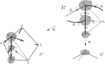
Figure 5.2. The local affine coordinates $\mathcal{U}_{1}$, $\mathcal{U}_{2}$ and their coordinate axes along singular lines with the projections to $Z_{1}^{sp}$ and $Z_{2}^{sp}$.

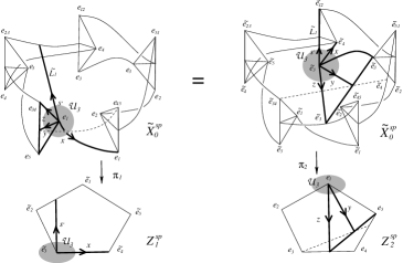
Figure 5.3. The local geometry $(\partial A_{1},\mathcal{U}_{3})$ with affine coordinates.

5.3.1. Resolution of $(3A_{1},\mathcal{U}_{1})$

We choose an affine coordinate $(s,t,u,v,\omega_{2,}\omega_{3,}\omega_{4,}\omega_{5})$ so that $s$, $t$ and $u$, respectively, coincide with the local parameters of the curves $Q_{5,}$ $\tilde{Q}_{1}$ and $\tilde{L}_{1},$ and also the origin represents the point $[\tilde{e}_{12}]\times[e_{1}]=[\tilde{e}_{1}-\frac{1}{a}\tilde{e}_{2}]\times[e_{1}].$ For this, we use the parametrization given in (5.2). Explicitly, we write the points on $Q_{5}$ by

$$\Bigl{[}a^{2}s\,\tilde{e}_{5}+(s+b)\tilde{e}_{12}\Bigr{]}\times\Bigl{[}se_{5}+e_{1}\Bigr{]} =\Bigl{[}\tilde{e}_{1}-\frac{1}{a}\tilde{e}_{2}-\frac{as}{s+b}\tilde{e}_{5}\Bigr{]}\times\Bigr{[}e_{1}+se_{5}\Bigr{]}$$

$$=\Bigl{[}\tilde{e}_{1}-\frac{1}{a}\tilde{e}_{2}+s\tilde{e}_{5}\Bigr{]}\times\Bigl{[}e_{1}-\frac{bs}{s+a}e_{5}\Bigr{]},$$

where we have changed $-\frac{as}{s+b}$ in the middle to $s$ using $Aut({\bf\mathbb{P}}^{1})$. Similarly, we can parametrize the points on $\tilde{Q}_{1}$ and $\tilde{L}_{1}$, respectively, by

$$\Bigl{[}\tilde{e}_{1}-\frac{1}{a}\tilde{e}_{2}+t\tilde{e}_{2}\Bigr{]}\times\Bigl{[}e_{1}-\frac{a}{b}t\,e_{2}+\frac{a}{b^{2}}t\,e_{3}\Bigr{]}\;,\;\;\Bigl{[}\tilde{e}_{1}-\frac{1}{a}\tilde{e}_{2}+u\tilde{e}_{3}\Bigr{]}\times\Bigl{[}e_{1}\Bigr{]}.$$

Introducing additional parameters $v,\omega_{2},\omega_{3},\omega_{4},\omega_{5}$, we take an affine coordinate of $\mathbb{C}^{4}\times\mathbb{C}^{4}\subset\mathbb{P}^{4}\times\mathbb{P}^{4}$ by

$$\Bigl{[}\tilde{e}_{1}+\bigl{(}t-\frac{1}{a}\bigr{)}\tilde{e}_{2}+u\tilde{e}_{3}+v\tilde{e}_{4}+s\tilde{e}_{5}\Bigr{]}\times\Bigl{[}e_{1}+\bigl{(}\omega_{2}-\frac{a}{b}t\bigr{)}e_{2}+\bigl{(}\omega_{3}+\frac{a}{b^{2}}t\bigr{)}e_{3}+\omega_{4}e_{4}+\bigl{(}\omega_{5}-\frac{bs}{s+a}\bigr{)}e_{5}\Bigr{]}.$$

In order to see the local geometry about the origin, we work in the local ring $\mathbb{C}[s,t,u,v,\omega_{2},..,\omega_{5}]_{m_{0}}$ with respect to the maximal ideal $m_{0}$ of the origin. Writing the defining equations of $\tilde{X}_{0}^{sp}$ in this ring, it is straightforward to see that the three equations (1st, 2nd and 5th equations in (2.3)) may be solved as $\omega_{2}=\omega_{5}=0$ and $\omega_{3}=-\frac{a^{3}tu}{b^{2}(1-at)}$. After substituting these into the remaining equation, we obtain

$$b^{3}(1-at)u\omega_{4}+at(u+av)(1-at-a^{2}u)=0,\;\omega_{4}(a+s)(as+v)-b^{2}sv=0.$$

Setting $\omega_{4}=w$, and focusing on the property near the origin, we have:

Proposition 5.5.

The local geometry $(3A_{1},\mathcal{U}_{1})$ near the singular point $[\tilde{e}_{12}]\times[e_{1}]$ is represented by the germ $(\{g_{1},g_{2}\},\mathbb{C}^{5})$ near the origin $(s,t,u,v,w)=(0,...,0)$ with

$$g_{1}=a\,t(u+a\,v)+b^{3}uw,\;\;g_{2}=aw(v+a\,s)-b^{2}sv.$$

Remark.

The coordinate $w=w_{4}$ has a special meaning related to the blow-up $\pi_{1}:\tilde{X}_{0}^{sp}\rightarrow Z_{1}^{sp}.$ In fact, in our affine coordinate $(s,t,u,v,\omega_{2,}\omega_{3,}\omega_{4,}\omega_{5})$, the exceptional divisor over the line $\tilde{q}_{1}$ can be written as

$$\Bigl{[}\tilde{e}_{1}-\frac{1}{a}\tilde{e}_{2}+t\tilde{e}_{2}\Bigr{]}\times\Bigl{[}e_{1}-\frac{a}{b}t\,e_{2}+\frac{a}{b^{2}}t\,e_{3}+\omega_{4}e_{4}\Bigr{]}\;\;(t,\omega_{4}\in\mathbb{C}).$$

Based on this, after eliminating the variable $w$ from the local equations by $\{g_{1},g_{2}\},$ we have a germ $(g_{3,}\mathbb{C}^{4})$ near the origin with

$$g_{3} =a^{2}\,t(u+a\,v)(v+a\,s)-b^{5}suv$$

$$=a^{3}\,stu+a^{4}\,stv+b^{5}\,suv+a^{2}\,tuv+a^{3}\,tv^{2},$$

where the polynomial $g_{3}$ coincides with the lowest oder terms of the defining (quintic) polynomial $Z_{1}^{sp}$ represented by the local parameters $(1,z_{2},z_{3},z_{4,}z_{5})=(1,t-\frac{1}{a},u,v,s)$. The $A_{1}$-singularity along $\tilde{Q}_{1}$ is the partial resolution of the $A_{2}$-singularity along $\tilde{q}_{1}$ in $Z_{2}^{sp}$. []

Let us consider the blowing-up $\tilde{\mathbb{C}}^{5}\rightarrow\mathbb{C}^{5}$ at the origin of the local geometry $(\{g_{1},g_{2}\},\mathbb{C}^{5})$, and denote the exceptional divisor by $E_{1}$. $E_{1}$ is the surface $\{g_{1}=g_{2}=0$} considered in $\mathbb{P}^{4}$ with the homogeneous coordinate $[S:T:U:V:W]$ corresponding to $(s,t,u,v,w)$.

Proposition 5.6.

$E_{1}$ is a singular del Pezzo surface of degree four with three nodal points, and has the Euler number $e(E_{1})=5$.

Proof.

The equations $g_{1}=g_{2}=0$ in $\mathbb{P}^{4}$ define a del Pezzo surface of degree 4. By evaluating the Jacobian ideal, it is immediate to see that this is singular at $[S:T:U:V:W]=[1:0:0:0:0],[0:1:0:0:0]$ and $[0:0:1:0:0]$, where the exceptional divisor $E_{1}$ intersects with the $s$-, $t$- and $u$-axes of $A_{1}$-singularities. Since $E_{1}$ is a singular Pezzo surface of degree 4 with three ordinary double points, it can be given as $\mathbb{P}^{2}$ blown-up at 5 points and then contracting three $(-2)$ curves [HW]. Therefore we have $e(E_{1})=8-3=5$.∎

Proposition 5.7.

After the blowing-up $(3A_{1},\mathcal{U}_{1})$ at the origin, the three singular lines separate from each other and intersect with $E_{1}$ at the three nodal points.

Proof.

We have chosen our coordinate of $\mathcal{U}_{1}$ so that $s$-, $t$-, $u$-axes coincide with the lines of $A_{1}$-singularity. The blowing-up $\tilde{\mathbb{C}}^{5}\rightarrow\mathbb{C}^{5}$ at the origin introduces the exceptional set $\mathbb{P}^{4}$, which separate the coordinate axes. Hence the blowing-up separates the $s$-, $t$-, $u$-axes of $A_{1}$-singularity from each other with introducing the exceptional divisor $E_{1}$. The intersection points of the (proper transforms of the) $s$-, $t$-, $u$-axes with $E_{1}$ coincides with the three nodal points of $E_{1}$. (This is similar to the case of the Barth-Nieto quintic [BaN].) ∎

Now, we blow-up all the 10 local geometries of type $(3A_{1},\mathcal{U}_{1})$ at their origins, and denote the blow-ups by $\varphi_{1}:\tilde{X}_{0}^{sp,(1)}\rightarrow\tilde{X}_{0}^{sp}$. Also we denote by $Q_{i}^{(1)},\tilde{Q}_{i}^{(1)},L_{i}^{(1)},\tilde{L}_{i}^{(1)}$ the proper transforms of the 20 lines $Q_{i},\tilde{Q}_{i},L_{i},\tilde{L}_{i}$ of $A_{1}$ singularity, respectively. Along these proper transforms of lines, we still have $A_{1}$ singularities. Also, these lines intersect at the origins of the 10 isomorphic local geometries of type $(2A_{1},\mathcal{U}_{2}^{(1)})$, which is isomorphic to $(2A_{1,}\mathcal{U}_{1})$ in $\tilde{X}_{0}^{sp}$. We also denote by $(\partial A_{1},\mathcal{U}_{3}^{(1)})\cong(\partial A_{1},\mathcal{U}_{3})$ the 10 isomorphic local geometries near the infinity points of the lines $L_{i}^{(1)},\tilde{L}_{i}^{(1)}$(see Fig. 5.2). The local geometries on each lines are now summarized as

(5.4) $$(\partial A_{1},\mathcal{U}_{3}^{(1)}),(2A_{1},\mathcal{U}_{2}^{(2)}) \text{ on each }\tilde{L}_{i}^{(1)},L_{i}^{(1)},$$

$$(2A_{1},\mathcal{U}_{1}^{(1)}) \text{ on each }\tilde{Q}_{i}^{(1)},Q_{i}^{(1)}.$$

5.3.2. Resolution of $(2A_{1},\mathcal{U}_{2}^{(1)})$

As in the previous case, we choose an affine coordinate $(s,t,u,v,\omega_{2},\omega_{3},\omega_{4},\omega_{5})$ centered at $[-a\,\tilde{e}_{12}+\tilde{e}_{3}]\times[e_{1}]$ with $s,t$ being along the lines $\tilde{L}_{1}^{(1)}$, $Q_{1}^{(1)}$ in $\tilde{X}_{0}^{sp,(1)}$. For this we parametrize the line $\tilde{L}_{1}^{(1)}$ by

$$\bigl{[}-a\tilde{e}_{12}+(1+s)\tilde{e}_{3}\bigr{]}\times[e_{1}]=\bigl{[}a^{2}\tilde{e}_{1}-a\tilde{e}_{2}+(1+s)\tilde{e}_{3}\bigr{]}\times[e_{1}],$$

and also the line $Q_{1}^{(1)}$ by

$$\bigl{[}a^{2}\tilde{e}_{1}+(1+t)\tilde{e}_{23}\bigr{]}\times\Bigl{[}e_{1}+\frac{1}{b}te_{2}\Bigr{]}=\bigl{[}a^{2}\tilde{e}_{1}-a(1+t)\tilde{e}_{2}+(1+t)\tilde{e}_{3}\bigr{]}\times\Bigl{[}e_{1}+\frac{t}{b}e_{2}\Bigr{]}.$$

Taking these forms into account, we introduce the affine coordinate by

$$\bigl{[}a^{2}\tilde{e}_{1}-a(1+t)\tilde{e}_{2}+(1+s+t)\tilde{e}_{3}+u\tilde{e}_{4}+v\tilde{e}_{5}\bigr{]}$$

$$\times\Bigl{[}e_{1}+\bigl{(}\omega_{2}+\frac{t}{b}\bigr{)}e_{2}+\omega_{3}e_{3}+\omega_{4}e_{4}+\omega_{5}e_{5}\Bigr{]}.$$

In the local ring $\mathbb{C}[s,t,u,v,\omega_{2},..,\omega_{5}]_{m_{0}}$, four of the five defining equations of $\tilde{X}_{0}^{sp,(1)}$ may be solved with respect to $\omega_{2},\omega_{3},\omega_{4},\omega_{5}$ and one equation leftover determines the germ about the origin.

Proposition 5.8.

The local geometry $(2A_{1},\mathcal{U}_{2}^{(1)})$ near the singular point $[-a\,\tilde{e}_{12}+\tilde{e}_{3}]\times[e_{1}]$ is represented by a germ $(h,\mathbb{C}^{4})$ near the origin $(s,t,u,v)=(0,0,0,0)$ with

(5.5) $$h=b^{5}uv+a^{3}\,stu+a^{4}\,stv+b^{5}suv+2b^{5}tuv.$$

We may derive the same form directly from the quintic equation of $Z_{1}^{sp}$ since the projection $\pi_{1}:\,\tilde{X}_{0}^{sp}\rightarrow Z_{1}^{sp}$ (composed with the blow-up $\tilde{X}_{0}^{sp,(1)}\rightarrow\tilde{X}_{0}^{sp})$ defines an isomorphism on the neighborhood $\mathcal{U}_{2}$, see Fig. 5.2. In the figure, the geometric meaning of the parameters $u$ and $v$ should be clear. By our choice of the coordinates, we have $A_{1}$-singularities along $s$- and $t$-axes, i.e., along the lines $\tilde{L}_{1}^{(1)}$ and $Q_{1}^{(1)}$, respectively. We will consider the blowing-up along $\tilde{L}_{1}^{(1)}$, which is locally described by the blowing-up $\mathbb{C}\times\tilde{\mathbb{C}}^{3}\rightarrow\mathbb{C}\times\mathbb{C}^{3}$ along the $s$-axis.

Proposition 5.9.

1) The exceptional divisor of the blow-up $\mathbb{C}\times\tilde{\mathbb{C}}^{3}\rightarrow\mathbb{C}\times\mathbb{C}^{3}$ of $(2\,A_{1},\mathcal{U}_{2}^{(1)})$ along the $s$-axis is a conic bundle over $s\in\mathbb{C}$ $(|s|\ll 1)$, which has a reducible fiber over $s=0$. This conic bundle is singular only at an ODP over $s=0$.

2) The conic bundle over $\mathbb{C}$ extends to a conic bundle $E_{2}\rightarrow\tilde{L}_{1}^{(1)}\cong\mathbb{P}^{1}$, which has reducible fibers over $s=0$ and $s=\infty$. This conic bundle is singular only at an ODP over $s=0,$ and also admits a section.

3) After the blowing-up of $(2A_{1},\mathcal{U}_{2}^{(1)})$, the singularity leftover near the local geometry is the $A_{1}$ singularity along the proper transform of the $t$-axis. The proper transform of $Q_{1}^{(1)}$ intersects with the conic bundle $E_{2}$ at the ODP over $s=0$.

Proof.

1) We introduce the coordinate $(s,[T,:U:V])$ for the exceptional set $\mathbb{C}\times\mathbb{P}^{2}$ of the blow-up $\mathbb{C}\times\tilde{\mathbb{C}}^{3}\rightarrow\mathbb{C}\times\mathbb{C}^{3}$. Then from the local equation of $(2A_{1},\mathcal{U}_{2})$, we have the equation of the exceptional divisor as

$$b^{5}UV+a^{3}sTU+a^{4}sTV+b^{5}sUV=0.$$

This defines a family of conics in $\mathbb{P}^{2}$ over $s\in\mathbb{C}\,(|s|\ll 1)$, which is reducible at $s=0$. Also we see that the conic bundle is singular only at an ODP over $s=0.$

2) To see the geometry of the exceptional divisor over $\mathbb{C}$($=\mathbb{P}^{1}\setminus\{s=\infty\}$), we need to have the equation (5.5) in all order in $s$ but with homogeneous of degree two for $t,u,v$. It is easy to have the equation from the defining equation of $Z_{1}^{sp}$. After some algebra, we have the equation for the exceptional divisor:

(5.6) $$(s+1)\left(b^{5}UV+a^{3}sTU+a^{4}sTV\right)=0,$$

which defines a conic bundle over $s\in\mathbb{C}\,(s\not=-1)$ with only one singular fiber over $s=0$. We see that $s=-1$ correspond to the intersection point of the exceptional divisor $E_{1}$ and the s-axis. Since this intersection point is one of the three nodal points on $E_{1}$, we see that the conic bundle extends to $s=-1$ with smooth fiber over it.

The point $s=\infty$ in the s-axis corresponds to the center of the local geometry $(\partial A_{1},\mathcal{U}_{3}^{(1)})$. We introduce the local parameters $s^{\prime}=\frac{1}{s},x,y,z$ to represent the relevant lines in this geometry, see Fig. 5.3. With other parameters $v_{1},v_{5}$ and $\omega_{2},\omega_{4}$, we consider the following affine coordinate centered at $[\tilde{e}_{3}]\times[e_{1}]$ of $\mathbb{P}^{4}\times\mathbb{P}^{4}:$

$$[(v_{1}-as^{\prime})\tilde{e}_{1}+s^{\prime}\tilde{e}_{2}+\tilde{e}_{3}+x\tilde{e}_{4}+v_{5}\tilde{e}_{5}]\times$$

$$[e_{1}+\omega_{2}e_{2}+(b^{2}y-z)e_{3}+(\omega_{4}-by+z)e_{4}+ye_{5}].$$

Writing the defining equations (2.3) in this coordinate, we can solve four equations with respect to $v_{1},v_{5},\omega_{2},\omega_{5}$ to obtain one equation $abxz+s^{\prime}(bxz+a^{4}yz-a^{4}by^{2})=0$ which describes the local geometry $(\partial A_{1},\mathcal{U}_{3}^{(1)})$ near the origin. Now we have the following local equation of the exceptional divisor of the blowing up along $s^{\prime}$-axis:

$$abXZ+s^{\prime}\left(bXZ+a^{4}YZ-a^{4}bY^{2}\right)=0\;\;(|s^{\prime}|\ll 1),$$

where $(s^{\prime},[X,Y,Z])$ represents the coordinates of the exceptional set $\mathbb{C}\times\mathbb{P}^{2}$ of the blow-up $\mathbb{C}\times\tilde{\mathbb{C}}^{3}\rightarrow\mathbb{C}\times\mathbb{C}^{3}$. From this equation, we see that the exceptional divisor is a conic bundle with reducible fiber over $s^{\prime}=0\,(s=\infty$) but smooth for $|s^{\prime}|\ll 1$.

Finally, from the equation (5.6), we see that $U=V=0$, for example, gives a section.

3) Let $(s,t,\tilde{u},\tilde{v})=(s,t,\frac{U}{T},\frac{V}{T})$ be the one of the affine coordinates of the blow-up. Then we have $u=\tilde{u}t,v=\tilde{v}t.$ Substituting these into the local equation $h$ of $(2A_{1},\mathcal{U}_{2}),$ i.e., for $|s|,|t|\ll 1$, we obtain

$$\tilde{h}=b^{5}\tilde{u}\tilde{v}+a^{3}s\tilde{u}+a^{4}s\tilde{v}+b^{5}s\tilde{u}\tilde{v}+2b^{5}t\tilde{u}\tilde{v}$$

with $h=t^{2}\tilde{h}$. If we set $t=0,$ then we have the equation of the exceptional divisor ($|s|\ll 1$) above. When we set $s=0,$ then we have $\tilde{h}=\tilde{u}\tilde{v}(b^{5}+2b^{5}t)$. This shows that the ODP of the exceptional divisor $E_{2}$ over $s=0$ merges to the $A_{1}$-singularity along the proper transform of the $t$-axis ( see Fig. 5.4). Since the singularity along the line $Q_{1}^{(1)}$ is of $A_{1}$-type except $t=0$, i.e., at the intersection $Q_{1}^{(1)}\cap\tilde{L}_{1}^{(1)}$, we now see that, near $t=0$, the singularity along the proper transform of $Q_{1}^{(1)}$ is of $A_{1}$-type. ∎

All the intersections of $Q_{i}^{(1)}$ and $\tilde{L}_{i}^{(1)}$ ($\tilde{Q}_{i}^{(1)}$ and $L_{i}^{(1)}$) have the local geometries isomorphic to $(2\,A_{1},\mathcal{U}_{2}^{(1)})$. We blow-up along all the 10 lines $\tilde{L}_{i}^{(1)}$ and $L_{i}^{(1)}$, and denote the blow-ups by $\varphi_{2}:\,\tilde{X}_{0}^{sp,(2)}\rightarrow\tilde{X}_{0}^{sp,(1)}$. We denote the proper transforms of the 10 lines $Q_{i}^{(1)}$ and $\tilde{Q}_{i}^{(1)}$, respectively, by $Q_{i}^{(2)}$ and $\tilde{Q}_{i}^{(2)}$.

5.3.3. Crepant Resolution $\tilde{X}_{0}^{*}\rightarrow\tilde{X}_{0}^{sp}$

We finally construct a crepant resolution.

Proposition 5.10.

1) All the singularities of $\tilde{X}_{0}^{sp,(2)}$ are along the non-intersecting 10 lines $Q_{i}^{(2)}$ and $\tilde{Q}_{i}^{(2)}$.

2) The singularities along $Q_{i}^{(2)}$ and $\tilde{Q}_{i}^{(2)}$ are of $A_{1}$-type. Blowing-up along each line of $Q_{i}^{(2)}$ and $\tilde{Q}_{1}^{(2)}$ resolves the singularity with introducing the exceptional divisor $E_{3}$ which is a $\mathbb{P}^{1}$-bundle with a section.

Proof.

1) Since each line of $Q_{i}$ and $\tilde{Q}_{i}$ intersects with others at the center of the local geometry $(3A_{1},\mathcal{U}_{1})$, it is clear that $Q_{i}^{(2)}$ and $\tilde{Q}_{i}^{(2)}$ are separated after the blow-ups (see Proposition 5.7).

2) By symmetry, it suffices to show the properties for a line, say $\tilde{Q}_{1}^{(2)}$. Note that $\tilde{Q}_{1}^{(2)}$ in $\tilde{X}_{0}^{sp,(2)}$ is given by the successive proper transform of the line $\tilde{Q}_{1}$ in $\tilde{X}_{0}^{sp}$ under the blow-ups of the local geometries, two $(3A_{1},\mathcal{U}_{1})$’s and one $(2A_{1},\mathcal{U}_{2})$ on the line. Therefore, the local geometry around $\tilde{Q}_{1}^{(2)}$ is isomorphic to that around the line $\tilde{Q}_{1}$ except the three centers of the blowing-ups on the line. We further note that the local geometry around the line $\tilde{Q}_{1}$ except the three centers is projected isomorphically to $Z_{2}^{sp}$ under the partial resolution $\pi_{2}:\tilde{X}_{0}^{sp}\rightarrow Z_{2}^{sp}$. The local geometry around $\pi_{2}(\tilde{Q}_{1})$ is easily analyzed by introducing the following affine coordinate:

$$[w_{1}:w_{2}:...:w_{5}]=[e_{1}+(u-bt)e_{2}+te_{3}+ve_{4}+we_{5}],$$

where $t$ parametrizes the line $\pi_{2}(\tilde{Q}_{1})$. Substituting this into the defining equation (2.6) of $Z_{2}^{sp}$and taking the polynomial of homogeneous degree up to two with respect to $u,v,w$ but all for $t$, we obtain

(5.7) $$bt\bigl{\{}a^{5}tvw-(1-b^{2}t)u(v+bw)\bigr{\}}=0,$$

which shows $A_{1}$-singularity along the $t$-axis except $t=0,\frac{1}{b^{2}}$ and $\infty$. These three values exactly correspond to the two local geometries $(3A_{1},\mathcal{U}_{1})$’s and one $(2A_{1},\mathcal{U}_{2})$ on the line $\tilde{Q}_{1}$, whose blowing-up we studied in Proposition 5.7 and Proposition 5.9. Combined with the results there, we conclude that the singularity along $\tilde{Q}_{1}^{(2)}$ is of $A_{1}$-type, and it is resolved by the blowing-up along the line with introducing an exceptional divisor $E_{3}$ which is isomorphic to a $\mathbb{P}^{1}$-bundle over the line. Also from the equation (5.7), it is easy to see that $E_{3}$ has a section (cf. Proposition 5.9 2) ). ∎

Let us now denote the blowing-up along the 10 lines by $\varphi_{3}:\tilde{X}_{0}^{sp,(3)}\rightarrow\tilde{X}_{0}^{sp,(2)}$. Defining $\tilde{X}_{0}^{*}:=\tilde{X}_{0}^{sp,(3)}$, we may summarize the whole process of the blowing-ups by

$$\varphi:\;\tilde{X}_{0}^{*}=\tilde{X}_{0}^{sp,(3)}\xrightarrow[\varphi_{3}]{}\tilde{X}_{0}^{sp,(2)}\xrightarrow[\varphi_{2}]{}\tilde{X}_{0}^{sp,(1)}\xrightarrow[\varphi_{1}]{}\tilde{X}_{0}^{sp},$$

where $\varphi:\tilde{X}_{0}^{*}\rightarrow\tilde{X}_{0}^{sp}$ represents the composition.

Theorem 5.11.

For $(a,b)\in(\mathbb{C}^{*})^{2}$ with non-vanishing discriminant (2.4), the blowing-up $\varphi:\tilde{X}_{0}^{*}\rightarrow\tilde{X}_{0}^{sp}$ is a crepant resolution and gives a smooth Calabi-Yau manifold with the Euler number $e(\tilde{X}_{0}^{*})=2(h^{1,1}(\tilde{X}_{0}^{*})-h^{2,1}(\tilde{X}_{0}^{*}))=100.$

Proof.

For the proof of $K_{\tilde{X}_{0}^{*}}\cong\mathcal{O}_{\tilde{X}_{0}^{*}}$, we show the existence of a nowhere vanishing holomorphic 3-form explicitly, although an abstract argument is possible. We first consider the blow-up, $\varphi_{1}:\tilde{X}_{0}^{sp,(1)}\rightarrow\tilde{X}_{0}^{sp}$ at the origin of the local geometries $(3A_{1},\mathcal{U}_{1})$. As before we introduce the affine coordinate $(s,t,u,v,w_{2},\cdots,w_{5})$. We start with the standard form of a nowhere vanishing holomorphic 3-form $\Omega(\tilde{X}_{0}^{sp})$ for the complete intersection Calabi-Yau variety $\tilde{X}_{0}^{sp}$ given in (6.1). In this affine coordinate, we have

$$\Omega(\tilde{X}_{0}^{sp})|_{\mathcal{U}_{1}}=Res_{f_{1}=\cdots=f_{5}=0}\Bigl{(}\frac{ds\wedge dt\wedge du\wedge dv\wedge dw_{2}\wedge\dots\wedge dw_{5}}{f_{1}f_{2}f_{3}f_{4}f_{5}}\Bigr{)}.$$

Evaluating the Jacobian $\frac{\partial(w_{2},w_{3},w_{5})}{\partial(f_{1},f_{2},f_{5})}=\frac{-a}{b^{2}(a+s)(1-at)}$, we calculate the residue as

(5.8) $$\Omega(\tilde{X}_{0}^{sp})|_{\mathcal{U}_{1}}=\frac{-1}{a}Res_{g_{1}=g_{2}=0}\Bigl{(}\frac{ds\wedge dt\wedge du\wedge dv\wedge dw}{g_{1}g_{2}}\Bigr{)},$$

where $w=w_{4}$ and $g_{1,}g_{2}$ are given in Proposition 5.5 (precisely $g_{1,}g_{2}$ here contain all higher order terms, but this does not affect the following arguments). Consider the blow-up $\varphi_{1}:\tilde{\mathbb{C}}^{5}\rightarrow\mathbb{C}^{5}$ at the origin, and one of the affine coordinate $(s,\tilde{t},\tilde{u},\tilde{v,}\tilde{w})=(s,\frac{T}{S},\frac{U}{S},\frac{V}{S},\frac{W}{S}$) with $t=\tilde{t}s,u=\tilde{u}s,v=\tilde{v}s,w=\tilde{w}s$. Then, pulling back the 3-form, it is immediate to have

(5.9) $$\varphi_{1}^{*}\Omega(\tilde{X}_{0}^{sp})\Bigl{|}_{\mathcal{U}_{1}^{(1)}}=\frac{-1}{a}Res_{\tilde{g}_{1}=\tilde{g}_{2}=0}\Bigl{(}\frac{ds\wedge d\tilde{t}\wedge d\tilde{u}\wedge d\tilde{v}\wedge d\tilde{w}}{\tilde{g}_{1}\tilde{g}_{2}}\Bigr{)},$$

where $g_{1}=s^{2}\tilde{g}_{1},g_{2}=s^{2}\tilde{g}_{2}$ and $\tilde{g}_{1}=\tilde{g}_{2}=0$ is the defining equation of the blow-up. Up to the non-vanishing constant, the right hand side is the holomorphic 3-form $\Omega(\tilde{X}_{0}^{sp,(1)})$ of $\tilde{X}_{0}^{sp,(1)}$. Calculations are similar for other affine coordinates, and we see that the pull-back $\varphi_{1}^{*}\Omega(\tilde{X}_{0}^{sp})$ coincides with $\Omega(\tilde{X}_{0}^{sp,(1)}),$ i.e., $\varphi_{1}$ is crepant. The next step $\varphi_{2}:\tilde{X}_{0}^{sp,(2)}\rightarrow\tilde{X}_{0}^{sp,(1)}$ has an effect on (5.9) as the blowing-up along the $s$-axis. Again, it is straightforward to see that $\Omega(\tilde{X}_{0}^{sp,(2)})\bigl{|}_{\mathcal{U}_{1}^{(2)}}=\varphi_{2}^{*}\Omega(\tilde{X}_{0}^{sp,(1)})\bigl{|}_{\mathcal{U}_{1}^{(2)}}$ holds up to a non-vanishing constant on all the affine coordinates. Doing similar calculations for the blow-up $\varphi_{3}$, we finally verify that $\Omega(\tilde{X}_{0}^{sp,(3)})\bigl{|}_{\mathcal{U}_{1}^{(3)}}=\varphi_{3}^{*}\Omega(\tilde{X}_{0}^{sp,(2)})\bigl{|}_{\mathcal{U}_{1}^{(3)}}$. Thus near the 10 points of the local geometry $(3A_{1,}\mathcal{U}_{1})$, we see that $\varphi:\tilde{X}_{0}^{*}\rightarrow\tilde{X}_{0}^{sp}$ is crepant.

For the local geometry $(2A_{1},\mathcal{U}_{2})$, since the first blow-up $\varphi_{1}$ has no effect, we start with $\Omega(\tilde{X}_{0}^{sp,(1)})\bigl{|}_{\mathcal{U}_{2}}=\Omega(\tilde{X}_{0}^{sp})\bigr{|}_{\mathcal{U}_{2}}$. As in the previous subsection, we introduce the affine coordinate $(s,t,u,v,w_{2},w_{3},w_{4})$. Evaluating the Jacobian $\frac{\partial(w_{2},w_{3},w_{4},w_{5})}{\partial(f_{1},f_{2},f_{3},f_{5})}$, we have

$$\Omega(\tilde{X}_{0}^{sp})\bigr{|}_{\mathcal{U}_{2}}=\frac{-1}{a}Res_{h=0}\Bigl{(}\frac{ds\wedge dt\wedge du\wedge dv}{h}\Bigr{)},$$

where $h$ is given in (5.5) (again, precisely $h$ should be understood with the higher order terms). Then $\varphi_{2}$ is the blow-up along the $s$-axis, see Proposition 5.9. Using one of the affine coordinate of the blow-up, $(s,t,\tilde{u},\tilde{v})=(s,t,\frac{U}{T},\frac{V}{T})$ with $u=\tilde{u}t,v=\tilde{v}t$, we evaluate the pull-back as

$$\varphi_{2}^{*}\Omega(\tilde{X}_{0}^{sp,(1)})\bigl{|}_{\mathcal{U}_{2}^{(2)}}=\frac{-1}{a}Res_{\tilde{h}=0}\Bigl{(}\frac{ds\wedge dt\wedge d\tilde{u}\wedge d\tilde{v}}{\tilde{h}}\Bigr{)},$$

with $h=t^{2}\tilde{h}$. Since $\tilde{h}=0$ is the local equation of the blow-up $\tilde{X}_{0}^{sp,(2)}$, we see that $\Omega(\tilde{X}_{0}^{sp,(2)})\bigl{|}_{\mathcal{U}_{2}^{(2)}}=\varphi_{2}^{*}\Omega(\tilde{X}_{0}^{sp,(1)})\bigl{|}_{\mathcal{U}_{2}^{(2)}}$ up to a non-vanishing constant. The next blow-up $\varphi_{3}$ is along the $t$-axis, and this is done locally by $(s,t,\tilde{u}^{\prime},\tilde{v}^{\prime})=(s,t,\frac{\tilde{U}}{\tilde{S}},\frac{\tilde{V}}{\tilde{S}})$ with $\tilde{u}=\tilde{u}^{\prime}s,\tilde{v}=\tilde{v}^{\prime}s.$ The local equation of the blow-up is given by $\tilde{h}^{\prime}=0$ with $\tilde{h}=s^{2}\tilde{h}^{\prime}$, and we have $\Omega(\tilde{X}_{0}^{sp,(3)})\bigl{|}_{\mathcal{U}_{2}^{(3)}}=\varphi_{3}^{*}\Omega(\tilde{X}_{0}^{sp,(2)})\bigl{|}_{\mathcal{U}_{2}^{(3)}}$, up to a non-vanishing constant. From the local equation $\tilde{h}^{\prime}=0$, we see that $\tilde{X}_{0}^{sp,(3)}=\tilde{X}_{0}^{*}$ is smooth. The calculations are valid for all the 10 points of the local geometry $(2A_{1},\mathcal{U}_{2})$.

Combined with the results for $(3A_{1,}\mathcal{U}_{1})$, we conclude that $\varphi:\tilde{X}_{0}^{*}\rightarrow\tilde{X}_{0}^{sp}$ is a crepant resolution.

Next we show that $\tilde{X}_{0}^{*}$ is a Calabi-Yau manifold, namely, i) $K_{\tilde{X}_{0}^{*}}\cong\mathcal{O}_{\tilde{X}_{0}^{*}}$ and ii) $h^{1}(\mathcal{O}_{\tilde{X}_{0}^{*}})=h^{2}(\mathcal{O}_{\tilde{X}_{0}^{*}})=0$. For the property i), we note that $K_{\tilde{X}_{0}^{sp}}\cong\mathcal{O}_{\tilde{X}_{0}^{sp}}$ since $\tilde{X}_{0}^{sp}$ is a complete intersection of $5$ divisors of $(1,1)$-type in $\mathbb{P}^{4}\times\mathbb{P}^{4}$. Then $K_{\tilde{X}_{0}^{*}}=\varphi^{*}K_{\tilde{X}_{0}^{sp}}\cong\mathcal{O}_{\tilde{X}_{0}^{*}}$ is immediate since $\varphi$ is crepant. For the second ii), we note that all the higher direct images $R^{i}\varphi_{*}\mathcal{O}_{\tilde{X}_{0}^{*}}\;(i>0)$ vanish by the Grauert-Riemenschneider vanishing since $\varphi$ is crepant. Then, by the Leray spectral sequence, we have $H^{i}(\mathcal{O}_{\tilde{X}_{0}^{*}})\cong H^{i}(\mathcal{O}_{\tilde{X}_{0}^{sp}})$$\,(i=1,2)$. Hence we have only to show that the r.h.s vanishes. Note that $\tilde{X}_{0}^{sp}$ is a complete intersection of $5$ divisors of $(1,1)$-type in $\mathbb{P}^{4}\times\mathbb{P}^{4}$, and consider the following Koszul resolution of $\mathcal{O}_{\tilde{X}_{0}^{sp}}$ :

$$0\to\mathcal{O}_{\mathbb{P}^{4}\times\mathbb{P}^{4}}(-5,-5)\to\mathcal{O}_{\mathbb{P}^{4}\times\mathbb{P}^{4}}(-4,-4)^{\oplus 4}\to\mathcal{O}_{\mathbb{P}^{4}\times\mathbb{P}^{4}}(-3,-3)^{\oplus 10}\to$$

$$\mathcal{O}_{\mathbb{P}^{4}\times\mathbb{P}^{4}}(-2,-2)^{\oplus 10}\to\mathcal{O}_{\mathbb{P}^{4}\times\mathbb{P}^{4}}(-1,-1)^{\oplus 5}\to\mathcal{O}_{\mathbb{P}^{4}\times\mathbb{P}^{4}}\to\mathcal{O}_{\tilde{X}_{0}^{sp}}\to 0.$$

As for the sheaves in this exact sequence except $\mathcal{O}_{\tilde{X}_{0}^{sp}}$, all the cohomology groups vanish except $H^{5}(\mathcal{O}_{\mathbb{P}^{4}\times\mathbb{P}^{4}}(-5,-5))\cong\mathbb{C}$ and $H^{0}(\mathcal{O}_{\mathbb{P}^{4}\times\mathbb{P}^{4}})\cong\mathbb{C}$ by the Kodaira vanishing theorem and the Serre duality. Now it is standard to see that $H^{2}(\mathcal{O}_{\tilde{X}_{0}^{sp}})\cong H^{5}(\mathcal{O}_{\mathbb{P}^{4}\times\mathbb{P}^{4}}(-5,-5))\cong\mathbb{C}$, $H^{0}(\mathcal{O}_{\tilde{X}_{0}^{sp}})\cong H^{0}(\mathcal{O}_{\mathbb{P}^{4}\times\mathbb{P}^{4}})\cong\mathbb{C}$ and $H^{i}(\mathcal{O}_{\tilde{X}_{0}^{sp}})\,(i=1,2)$ vanish.

Figure 5.4. Exceptional divisors $E_{1},E_{2},E_{3}$ of the blowing-ups $\varphi_{1},\varphi_{2},\varphi_{3}$, respectively. Only the local geometries around the line $\tilde{L}_{1}$ in $\tilde{X}_{0}^{sp}$ are depicted.

For the calculation of the Euler number, let us first note that we have $e(\tilde{X}_{0}^{sp})=e(Z_{2}^{sp})+5\times\bigl{(}e(\mathbb{P}^{2})-1\bigr{)}=-10+10=0$. This follows form Proposition 3.4 and Proposition 5.2, see also Fig. 5.1. Now we note that, under the blow-up, the origin of $(3A_{1,}\mathcal{U}_{1})$ is replaced by the exceptional divisor $E_{1}$ with its Euler number $e(E_{1})=5.$ Similarly for $(2\,A_{1},\mathcal{U}_{2}^{(1)})$, one line is replaced by a conic bundle $E_{2}$ over $\mathbb{P}^{1}$ with two reducible fibers, hence $e(E_{2})=6$. Since we have 10 isomorphic geometries for $(3A_{1,}\mathcal{U}_{1})$ and 10 for $(2\,A_{1},\mathcal{U}_{2}^{(1)})$, taking into account the final blow-ups of 10 lines, we evaluate the Euler number $e(\tilde{X}_{0}^{*}$) as

$$e(\tilde{X}_{0}^{*}) =10\times\bigl{(}e(E_{1})-1\bigr{)}+10\times\bigl{(}e(E_{2})-e(\mathbb{P}^{1})\bigr{)}+10\times\bigl{(}e(E_{3})-e(\mathbb{P}^{1})\bigr{)}$$

$$=40+10\times(6-2)+10\times 2=100.$$

∎

5.4. Hodge numbers

Recall that the crepant resolution is obtained as the composite of the blowing-ups $\varphi_{1}:\tilde{X}_{0}^{sp,(1)}\rightarrow\tilde{X}_{0}^{sp}$, $\varphi_{2}:\tilde{X}_{0}^{sp,(2)}\rightarrow\tilde{X}_{0}^{sp,(1)}$, $\varphi_{3}:\tilde{X}_{0}^{sp,(3)}\rightarrow\tilde{X}_{0}^{sp,(2)}$. The first blow-up $\varphi_{1}$ introduces the exceptional divisors $E_{1}(=:E_{1}^{(1)})$ in $\tilde{X}_{0}^{sp,(1)}$ which is a del Pezzo surfaces of degree 4 with three lines are contracted to three points. One of the three points is resolved in the proper transform $E_{1}^{(2)}$ under $\varphi_{2}$, and the other two are resolved in the proper transform $E_{1}^{(3)}$ under $\varphi_{3}$. Similarly, the resolution $\varphi_{2}$ introduces the conic bundle $E_{2}(=:E_{2}^{(2)})$ over $\mathbb{P}^{1}$ which has an ordinary double point (over $s=0$), and $\varphi_{3}$ resolves this singularity to have smooth ruled surface $E_{2}^{(3)}$ in $\tilde{X}_{0}^{sp,(3)}$. The final blow-up $\varphi_{3}$ introduces the divisor $E_{3}=E_{3}^{(3)}$ which is a $\mathbb{P}^{1}$-bundle over $\mathbb{P}^{1}$ with a section. Note that all these divisors $E_{1}^{(3)},E_{2}^{(3)}$ and $E_{3}^{(3)}$ are smooth in $\tilde{X}_{0}^{sp,(3)}=\tilde{X}_{0}^{*}$.

In this subsection, following [HSvGvS], we apply the Weil conjecture to determine the Hodge numbers of the resolution $\tilde{X}_{0}^{*}.$ We set our parameters to $a=b=1$ and consider the mod $p$ reduction of $\tilde{X}_{0}^{*}.$ We write $\mathbb{F}_{p}=\mathbb{Z}/p\mathbb{Z}$.

Lemma 5.12.

For all but finite primes, the reduction of $\tilde{X}_{0}^{*}$ modulo $p$ is smooth over $\mathbb{F}_{p}$.

Proof.

The smoothness of $\tilde{X}_{0}^{*}$ in the tori $(\mathbb{C}^{*})^{4}\times(\mathbb{C}^{*})^{4}$ follows from the discriminant (in Proposition 2.3) $dis(\tilde{X}_{0}^{sp}|_{(\mathbb{C}^{*})^{4}})=3\times 11^{3}$ for $a=b=1.$ The exceptional divisors $E_{1},E_{2}$ of the blowing-ups $\varphi_{1}$ and $\varphi_{2}$, respectively, are blown-up to smooth surfaces $E_{1}^{(3)}$ and $E_{2}^{(3)}$ in $\tilde{X}_{0}^{*}$, hence the resolution $\tilde{X}_{0}^{*}$ is smooth over $\mathbb{F}_{p}$ except finite primes $p$. ∎

Let $\tilde{X}_{0}^{*}(\mathbb{F}_{p})$ be the set of points in $\tilde{X}_{0}^{*}$ which are rational over $\mathbb{F}_{p}.$ We use the Lefschetz fixed point formula due to Grothendieck,

(5.10) $$\#\tilde{X}_{0}^{*}(\mathbb{F}_{p})=1-t_{1}+t_{2}-t_{3}+t_{4}-t_{5}+t_{6},$$

with $t_{j}=\text{tr (\text{Frob}}_{p}^{*}\bigl{|}H_{\acute{e}t}^{j}(\tilde{X}_{0}^{*},\mathbb{Q}_{\ell}))$ and $\text{Frob}_{p}:\tilde{X}_{0}^{*}\rightarrow\tilde{X}_{0}^{*}$ the Frobenius morphism. Since $\tilde{X}_{0}^{*}$ is a Calabi-Yau threefold, we have $t_{0}=1,t_{1}=t_{5}=0,t_{6}=p^{3}$. By the Weil conjecture (see [Har, Appendix C] for example), the eigenvalues of $\text{Frob}_{p}$ on $H_{\acute{e}t}^{j}(\tilde{X}_{0}^{*},\mathbb{Q}_{\ell})$ are algebraic integers, which do not dependent on $\ell,$ with absolute values $p^{j/2}$. Also, by the Weil conjecture again, $t_{j}$’s are (ordinary) integers and satisfy $|t_{j}|\leq b_{j}(\tilde{X}_{0}^{*})\;p^{j/2}$. We derive the following property following the arguments in [HSvGvS, Prop. 2.4] made for the Barth-Nieto quintic.

Proposition 5.13.

For every good prime $p$, all eigenvalues of $\text{Frob}_{p}$ on $H_{\acute{e}t}^{2}(\tilde{X}_{0}^{*},\mathbb{Q}_{\ell})$ are equal to $p$.

Proof.

Due to Lemma 5.14 below, we can use the Lefschetz hyperplane theorem [FK, Corollary I.9.4] and have the claimed property for $\tilde{X}_{0}^{sp}$. Then from the Leray spectral sequence associated to $\varphi_{1}:\tilde{X}_{0}^{sp,(1)}\rightarrow\tilde{X}_{0}^{sp},$ we obtain the claimed property for $\tilde{X}_{0}^{sp,(1)}$ (see [HSvGvS, Lemma 2.16]). To go further to $\tilde{X}_{0}^{sp,(2)}$, we use the Leray spectral sequence associated to $\varphi_{2}:\tilde{X}_{0}^{sp,(2)}\rightarrow\tilde{X}_{0}^{sp,(1)}$,

$$E_{2}^{j,2-j}=H_{\acute{e}t}^{j}(\tilde{X}_{0}^{sp,(1)},R^{2-j}{\varphi_{2}}_{*}(\mathbb{Q}_{\ell}))\Rightarrow H_{\acute{e}t}^{2}(\tilde{X}_{0}^{sp,(2)},\mathbb{Q}_{\ell}),$$

where $E_{2}^{2,0}=H_{\acute{e}t}^{2}(\tilde{X}_{0}^{sp,(1)},\mathbb{Q}_{\ell}),\;E_{2}^{1,1}=0$ and $E_{2}^{0,2}=H_{\acute{e}t}^{2}(\tilde{X}_{0}^{sp,(1)},R^{2}{\varphi_{2}}_{*}(\mathbb{Q}_{\ell}))$. Due to Lemma 5.15 below, we have the claimed property for $E_{2}^{0,2}$ as well as $E_{2}^{2,0}$, hence for $H_{\acute{e}t}^{2}(\tilde{X}_{0}^{sp,(2)},\mathbb{Q}_{\ell})$, too. To go from $\tilde{X}_{0}^{sp,(2)}$ to $\tilde{X}_{0}^{sp,(3)}=\tilde{X}_{0}^{*}$, we can use the argument in [ibid, Lemma 2.16] since the exceptional divisor $E_{3}(=E_{3}^{(3)})$ of $\varphi_{3}:\tilde{X}_{0}^{sp,(3)}\rightarrow\tilde{X}_{0}^{sp,(2)}$ is a $\mathbb{P}^{1}$-bundle over $\mathbb{P}^{1}$. Thus we obtain the claimed property for $H_{\acute{e}t}^{2}(\tilde{X}_{0}^{*},\mathbb{Q}_{\ell})$.∎

Lemma 5.14.

Consider $\tilde{X}_{0}^{sp}$ as the linear section $(\mathbb{P}^{4}\times\mathbb{P}^{4})\cap H_{1}\cap...\cap H_{5}$ in $\mathbb{P}^{24}$ by the Segre embedding with $H_{k}$ representing the defining equation $f_{k}=\,^{t}zA_{k}w\,(k=1,...,5)$. Then for all but finite primes $p$, there exists a sequence linear forms $H_{1}^{\prime},H_{2}^{\prime},...,H_{5}^{\prime}$ over $\mathbb{Z}$ with the following properties over $\mathbb{F}_{p}$: 1) Sing$(X_{i-1})$$\subset X_{i}$ holds for $i=2,..,5,$ where $X_{i}=(\mathbb{P}^{4}\times\mathbb{P}^{4})\cap H_{1}^{\prime}\cap..\cap H_{i}^{\prime}$ and Sing$(X_{i-1})$ is the singular loci of $X_{i-1}$. 2) $X_{5}=\tilde{X}_{0}^{sp}$.

Proof.

Since $f_{k}$’s are defined over $\mathbb{Z}$, it suffices to have the properties 1) and 2) over $\mathbb{C}$. We can verify explicitly that the sequence $H_{1}^{\prime},H_{2}^{\prime},...,H_{5}^{\prime}$ corresponding to $f_{1}+f_{3}+f_{5},f_{2}+f_{4},3f_{2}+f_{5},5f_{3}+f_{4},f_{5}$ satisfies the desired properties over $\mathbb{C}$. ∎

Lemma 5.15.

All the eigenvalues of $\mathrm{Frob}_{p}$ on $H_{\acute{e}t}^{0}(\tilde{X}_{0}^{sp,(1)},R^{2}{\varphi_{2}}_{*}(\mathbb{Q}_{l}))$ are equal to $p$ for every good prime $p$.

Proof.

Set $\rho_{1}:=\varphi_{2}|_{E_{2}^{(2)}}$. First note that $H_{\acute{e}t}^{0}(\tilde{X}_{0}^{sp,(1)},R^{2}{\varphi_{2}}_{*}\mathbb{Q}_{l})\simeq H_{\acute{e}t}^{0}(E_{2}^{(2)},R^{2}{\rho_{1}}_{*}\mathbb{Q}_{l})$. Let $\rho_{2}\colon E_{2}^{(3)}\to E_{2}^{(2)}$ be the blow-up of the ordinary double point of $E_{2}^{(2)}$ on the fiber of $E_{2}^{(2)}\to\mathbb{P}^{1}$ over $s=0$ (see Proposition 5.9). Denote by $\rho$ the composite of $\rho_{2}$ and $\rho_{1}$. We have the spectral sequence:

(5.11) $$E_{2}^{i,j}:=R^{i}{\rho_{1}}_{*}(R^{j}{\rho_{2}}_{*}\mathbb{Q}_{l})\Longrightarrow R^{i+j}\rho_{*}(\mathbb{Q}_{l}).$$

By standard calculations, we have

• $E_{2}^{2,0}=R^{2}{\rho_{1}}_{*}(\mathbb{Q}_{l}$).

• Since the nontrivial fiber of $\rho_{2}$ is a $\mathbb{P}^{1}$, we have $R^{1}{\rho_{2}}_{*}(\mathbb{Q}_{l})=0$. Hence $E_{2}^{1,1}=0$.

• $E_{2}^{0,2}\simeq H_{\acute{e}t}^{2}(\mathbb{P}^{1},\mathbb{Q}_{l})$, where $\mathbb{P}^{1}$ is the nontrivial fiber of $\rho_{2}$, and we consider $H_{\acute{e}t}^{2}(\mathbb{P}^{1},\mathbb{Q}_{l})$ as a skyscraper sheaf supported on $s=0$.

Then, by standard properties of the spectral sequence, we have the following exact sequence:

$$0\to R^{2}{\rho_{1}}_{*}(\mathbb{Q}_{l})\to R^{2}{\rho}_{*}(\mathbb{Q}_{l})\to H_{\acute{e}t}^{2}(\mathbb{P}_{1},\mathbb{Q}_{l})\to 0.$$

Therefore, to show the claimed property for $H_{\acute{e}t}^{0}(\tilde{X}_{0}^{sp,(1)},R^{2}{\varphi_{2}}_{*}(\mathbb{Q}_{l}))$, we have only to show that the claimed property holds for $H_{\acute{e}t}^{0}(E_{2}^{(2)},R^{2}{\rho}_{*}(\mathbb{Q}_{l}))$.

Let $\rho_{3}\colon E_{2}^{(3)}\to E_{2}^{\prime}$ be the contraction of three $(-1)$-curves on $E_{2}^{(3)}$, two of which are the strict transforms of the components of the fiber of $E_{2}^{(2)}\to\mathbb{P}^{1}$ over $s=0$, and the remaining one of which is one component of the fiber of $E_{2}^{(2)}\to\mathbb{P}^{1}$ over $s=\infty$ (see Proposition 5.9). Denote by $\rho_{4}\colon E_{2}^{\prime}\to\mathbb{P}^{1}$ the natural induced morphism, which defines a $\mathbb{P}^{1}$-bundle structure. We have the spectral sequence:

(5.12) $$R^{i}{\rho_{4}}_{*}(R^{j}{\rho_{3}}_{*}(\mathbb{Q}_{l}))\Longrightarrow R^{i+j}\rho_{*}(\mathbb{Q}_{l}).$$

By similar considerations to those for (5.11), we have the following exact sequence:

$$0\to R^{2}{\rho_{4}}_{*}(\mathbb{Q}_{l})\to R^{2}{\rho}_{*}(\mathbb{Q}_{l})\to H_{\acute{e}t}^{2}(\mathbb{P}^{1},\mathbb{Q}_{l})^{\oplus 3}\to 0.$$

Note that all eigenvalues of $\mathrm{Frob}_{p}$ on $H_{\acute{e}t}^{2}(\mathbb{P}_{1},\mathbb{Q}_{l})^{\oplus 3}$ are equal to $p$. Therefore, to show that the claimed property holds for $H_{\acute{e}t}^{0}(E_{2}^{(2)},R^{2}{\rho}_{*}(\mathbb{Q}_{l}))$, we have only to show that the claimed property holds for $H_{\acute{e}t}^{0}(E_{2}^{\prime},R^{2}{\rho_{4}}_{*}(\mathbb{Q}_{l}))$.

Now we consider the Leray spectral sequence:

$$H_{\acute{e}t}^{i}(\mathbb{P}^{1},R^{j}{\rho_{4}}_{*}(\mathbb{Q}_{l}))\Longrightarrow H_{\acute{e}t}^{i+j}(E_{2}^{\prime},\mathbb{Q}_{l}).$$

Since $\rho_{4}$ is a $\mathbb{P}^{1}$-bundle, we have $R^{1}{\rho_{4}}_{*}(\mathbb{Q}_{l})=0$. Therefore, in a similar way as above, we have the following exact sequence:

$$0\to H_{\acute{e}t}^{2}(\mathbb{P}^{1},\mathbb{Q}_{l})\to H_{\acute{e}t}^{2}(E_{2}^{\prime},\mathbb{Q}_{l})\to H_{\acute{e}t}^{0}(E_{2}^{\prime},R^{2}{\rho_{4}}_{*}(\mathbb{Q}_{l}))\to 0.$$

Since $\rho_{1}\colon E_{2}^{(2)}\to\mathbb{P}^{1}$ has a section defined over $\mathbb{Q}$, due to 2) in Proposition 5.9 applied to $a,b\in\mathbb{Z}$, so does $\rho_{4}\colon E_{2}^{\prime}\to\mathbb{P}^{1}$. Therefore $H_{\acute{e}t}^{2}(E_{2}^{\prime},\mathbb{Q}_{l})$ is generated by the classes of divisors defined over $\mathbb{Q}$, which are a section and a fiber. Hence all eigenvalues of $\mathrm{Frob}_{p}$ on $H_{\acute{e}t}^{2}(E_{2}^{\prime},\mathbb{Q}_{l})$ are equal to $p$ [vGN], and then the claimed property holds for $H_{\acute{e}t}^{0}(E_{2}^{\prime},R^{2}{\rho_{4}}_{*}(\mathbb{Q}_{l}))$.

∎

Figure 5.5.

From the Proposition 5.13 and the fixed point formula (5.10), we have

(5.13) $$\bigl{|}1+(50+h^{21})(p+p^{2})+p^{3}-\#\tilde{X}_{0}^{*}(\mathbb{F}_{p})\bigr{|}\leq(2+2\,h^{21})p^{\frac{3}{2}},$$

where we have used $b_{2}=b_{4}$ by the Poincaré duality and also expressed $b_{2}=h^{11}=(50+h^{21})$ from $e(\tilde{X}_{0}^{*})=2(h^{11}-h^{21})=100.$

Proposition 5.16.

The number of rational points $\#\tilde{X}_{0}^{*}(\mathbb{F}_{p})$ is given by

$$\#\tilde{X}_{0}^{*}(\mathbb{F}_{p})=\#Z_{2}^{sp}(\mathbb{F}_{p})+10\times\#E_{1}(\mathbb{F}_{p})+30\,p^{2}+40\,p-10,$$

where $\#Z_{2}^{sp}(\mathbb{F}_{p})$ and $\#E_{1}(\mathbb{F}_{p})$ are the numbers of rational points over $\mathbb{F}_{p}$ for the determinantal quintic (2.6) and the singular del Pezzo surface in Proposition 5.5, respectively, with $a=b=1$.

Proof.

The projection $\pi_{2}:\tilde{X}_{0}^{sp}\rightarrow Z_{2}^{sp}$ is isomorphic outside the coordinate lines $q_{i}$ ( see Fig. 5.1). Since the fibers over the coordinate point $[e_{i}]$ and $q_{i}\setminus\{[e_{i}],[e_{i+1}]\}$ are $\mathbb{P}^{2}$ and $\mathbb{P}^{1},$ respectively, we obtain

$$\#\tilde{X}_{0}^{sp}(\mathbb{F}_{p}) =\#Z_{2}^{sp}(\mathbb{F}_{p})+5\times(N_{\mathbb{P}^{2}}-1)+5\times(N_{\mathbb{P}^{1}}-1)(N_{\mathbb{P}^{1}}-2)$$

$$=\#Z_{2}^{sp}(\mathbb{F}_{p})+10p^{2},$$

where $N_{\mathbb{P}^{2}}=p^{2}+p+1$ and $N_{\mathbb{P}^{1}}=p+1$, respectively, count the number of rational points in $\mathbb{P}^{2}$ and $\mathbb{P}^{1}$ over $\mathbb{F}_{p}$. We count the number of rational points on the conic bundle $E_{2}$ (with two reducible fibers) over $\mathbb{P}^{1}$ as

$$\#E_{2}(\mathbb{F}_{p})=(p+1)(p-1)+(2p+1)\times 2=p^{2}+4p+1.$$

The counting for $E_{3}$ is given by $\#E_{3}(\mathbb{F}_{p})=(p+1)^{2}$. Now summarizing all, we obtain

$$\#\tilde{X}_{0}^{*}(\mathbb{F}_{p}) =\#\tilde{X}_{0}^{sp}(\mathbb{F}_{p})+10\times\bigl{(}\#E_{1}(\mathbb{F}_{p})-1\bigr{)}$$

$$\qquad\qquad+10\times\bigl{(}\#E_{2}(\mathbb{F}_{p})-(p+1)\bigr{)}+10\times\bigl{(}\#E_{3}(\mathbb{F}_{p})-(p+1)\bigr{)}$$

$$=\#Z_{2}^{sp}(\mathbb{F}_{p})+10\times\#E_{1}(\mathbb{F}_{p})+30\,p^{2}+40\,p-10.$$

∎

Writing a straightforward computer codes, we have evaluated the number $\#\tilde{X}_{0}^{*}(\mathbb{F}_{p})$. After the computations in several minutes, we verify the inequality (5.13) for $p\leq 97$ with $h^{2,1}=2$ or $3.$ For example, we obtain $\#\tilde{X}_{0}^{*}(\mathbb{F}_{p})=669880,\,1118250$ and 1408330 for $p=73,\,89$ and $97$, respectively. We observe that the inequality (5.13) holds only if $h^{2,1}=2$ for $p=59,61,71,73,89,97$. Also we can verify that these are good primes by analyzing the Jacobian ideals over the field $\mathbb{F}_{p}.$ Since the inequality holds for all good primes, we conclude that:

Theorem 5.17.

The smooth Calabi-Yau manifold $\tilde{X}_{0}^{*}$ has Hodge numbers;

$$h^{1,1}(\tilde{X}_{0}^{*})=52,\;\;\;h^{2,1}(\tilde{X}_{0}^{*})=2.$$

In particular this is mirror symmetric to the generic complete intersection $\tilde{X}_{0}$ with $h^{1,1}(\tilde{X}_{0})=2,\,h^{2,1}(\tilde{X}_{0})=52$.

 

6. Picard-Fuchs equations and monodromy matrices

6.1. Picard-Fuchs differential equations

We consider a family of Calabi-Yau manifolds $\tilde{X}_{0}^{*}$ defined over $(\mathbb{C}^{*})^{2}\ni(a,b)$. Here we briefly introduce a natural compactification of $(\mathbb{C}^{*})^{2}$ to $\mathbb{P}^{2}$ which follows from the differential equations satisfied by the period integrals, see [HKTY] and [HT] for details. To formulate the set of differential operators, we slightly modify the defining equations (2.3) to

$$f_{i}=c_{i}z_{i}w_{i}+a_{i}z_{i+1}w_{i}+b_{i}z_{i}w_{i+1}\;\;(i=1,...,5),$$

where the indices are considered modulo five as before. Clearly, the original forms are recovered by setting $a_{i}=a,b_{i}=b,c_{i}=1$. Since we have $\tilde{X}_{0}^{*}|_{(\mathbb{C}^{*})^{4}\times(\mathbb{C}^{*})^{4}}\simeq\tilde{X}_{0}^{sp}|_{(\mathbb{C}^{*})^{4}\times(\mathbb{C}^{*})^{4}}$ for $(\mathbb{C}^{*})^{4}\times(\mathbb{C}^{*})^{4}\subset\mathbb{P}^{4}\times\mathbb{P}^{4}$, a holomorphic 3-form of the crepant resolution $\tilde{X}_{0}^{*}$ may be given by the corresponding 3-form of $\tilde{X}_{0}^{sp}$ if the 3-cycles of the period integrals are contained in $(\mathbb{C}^{*})^{4}\times(\mathbb{C}^{*})^{4}$. For the complete intersection $\tilde{X}_{0}^{sp}$, the following expression of a holomorphic 3-form is well-known [Gr]:

(6.1) $$\Omega(\tilde{X}_{0}^{sp})=Res_{f_{1}=...=f_{5}=0}\left(\frac{d\mu_{1}\wedge d\mu_{2}}{f_{1}f_{2}\cdots f_{5}}\right),$$

where

$$d\mu_{1}=-\sum_{i=1}^{5}(-1)^{i}z_{i}dz_{1}\wedge\cdots\wedge\widehat{dz_{i}}\wedge\cdots\wedge dz_{5},$$

and similar definition for $d\mu_{2}$ with the coordinates $w_{k}$’s . The period integral $\int_{\Gamma}\Omega(\tilde{X}_{0}^{*})$ for a 3-cycle $\Gamma\in H_{3}(\tilde{X}_{0}^{*},\mathbb{Z})$ satisfies a system of differential equations, the so-called Picard-Fuchs differential equations, see [Mo], [DGJ] for example. In the present case, assuming that the cycle $\Gamma$ is contained in $(\mathbb{C}^{*})^{4}\times(\mathbb{C}^{*})^{4}$, we can describe the system by noting rather trivial algebraic relations represented in terms of differential operators, e.g.,

$$\left\{\frac{\partial\;}{\partial c_{1}}\frac{\partial\;}{\partial c_{2}}\frac{\partial\;}{\partial c_{3}}\frac{\partial\;}{\partial c_{4}}\frac{\partial\;}{\partial c_{5}}-\frac{\partial\;}{\partial a_{1}}\frac{\partial\;}{\partial a_{2}}\frac{\partial\;}{\partial a_{3}}\frac{\partial\;}{\partial a_{4}}\frac{\partial\;}{\partial a_{5}}\right\}\Omega(\tilde{X}_{0}^{sp})=0,$$

which represents $\Pi_{i=1}^{5}z_{i}w_{i}-\Pi_{i=1}^{5}z_{i+1}w_{i}=0$. We should also note that the holomorphic 3-form is invariant under the $(\mathbb{C}^{*})^{4}$-action $z_{i}\mapsto t_{i}z_{i}$, $(t_{1}t_{2}\cdots t_{5}=1)$ and similar $(\mathbb{C}^{*})^{4}$-action on the coordinates $w_{i}$’s. We note further that $\Omega(\tilde{X}_{0}^{sp})$ has a simple scaling property under $f_{i}\mapsto r_{i}f_{i}$ $(r_{i}\in\mathbb{C}^{*})$. All these properties of invariance (or covariance) may be expressed by the corresponding linear differential operators, and may be used to reduce the enlarged parameters to the original $a$ and $b$. The system of differential operators which we obtain in this way is an example of the Gel’fand-Kapranov-Zelevinski (GKZ) system [GKZ] for which a natural compactification of the parameters is known. In the present case, from the $\mathbb{C}^{*}$-actions above and the form of the defining equations (2.3), it is rather easy to deduce that $(\mathbb{C}^{*})^{2}\ni(a,b)$ is compactified to $\mathbb{P}^{2}\ni[a^{5}:b^{5}:1]$. According to the mirror symmetry calculations formulated in [HKTY], we actually come to the affine charts $\{(x,y),\mathcal{A}_{0}\},\{(x_{1},y_{1}),\mathcal{A}_{1}\}$ and $\{(x_{2},y_{2}),\mathcal{A}_{2}\}$ defined by

$$x=-a^{5},y=-b^{5};\;x_{1}=-\frac{b^{5}}{a^{5}},y_{1}=-\frac{1}{a^{5}};\;x_{2}=-\frac{a^{5}}{b^{5}},y_{2}=-\frac{1}{b^{5}}.$$

Up to signs, these relations are in accord with the standard relations $[a^{5}:b^{5}:1]=[1:\frac{b^{5}}{a^{5}}:\frac{1}{a^{5}}]=[\frac{a^{5}}{b^{5}}:1:\frac{1}{b^{5}}]$ of the affine coordinates of $\mathbb{P}^{2}$. The extra minus signs follows from the general definition given in [HKTY].

Proposition 6.1.

On the affine chart $\{(x,y),\mathcal{A}_{0}\}$, the following differential operators determine the period integrals as the solutions:

$$\mathcal{D}_{1}(x,y) =2\theta_{x}^{3}-3\theta_{x}^{2}\theta_{y}+3\theta_{x}\theta_{y}^{2}-2\theta_{y}^{3}-(\theta_{x}+\theta_{y})^{2}\bigl{\{}(2\theta_{x}+3\theta_{y})x-(3\theta_{x}+2\theta_{y})y\bigr{\}},$$

$$\mathcal{D}_{2}(x,y) =2\theta_{x}^{2}-3\theta_{x}\theta_{y}+2\theta_{y}^{2}-(2\theta_{x}^{2}+7\theta_{x}\theta_{y}+7\theta_{y}^{2})x-(7\theta_{x}^{2}+7\theta_{x}\theta_{y}+2\theta_{y}^{2})y,$$

where $\theta_{x}=x\frac{\partial\;}{\partial x},\theta_{y}=y\frac{\partial\;}{\partial y}.$ On the other affine charts the differential operators are given by the following gauge transforms of the operators $\mathcal{D}_{1}(x,y),\mathcal{D}_{2}(x,y)$:

$$\mathcal{D}^{\prime}_{1}(x_{1},y_{1}):=x_{1}\mathcal{D}_{1}(x_{1},y_{1})x_{1}^{-1},\;\mathcal{D}^{\prime}_{2}(x_{1},y_{1}):=\mathcal{D}_{2}(x_{1},y_{1})\;\;\text{on\;}\{(x_{1},y_{1}),\mathcal{A}_{1}\}$$

and

$$\mathcal{D}^{\prime\prime}_{1}(x_{2},y_{2}):=x_{2}\mathcal{D}_{1}(x_{2},y_{2})x_{2}^{-1},\;\mathcal{D}^{\prime\prime}_{2}(x_{2},y_{2}):=\mathcal{D}_{2}(x_{2},y_{2})\;\;\text{on}\;\{(x_{2},y_{2}),\mathcal{A}_{2}\}.$$

Proof.

For the derivation of the differential operators $\mathcal{D}_{1},\mathcal{D}_{2}$, we refer to [HKTY]. Also see Prop.2.6 in [HT]. Note that the parameters $(a_{i},b_{i},c_{i})$ in [HT, (2.6) ] should be read as $(c_{i},a_{i},b_{i})$ here (see the defining equations $f_{i}$ ). ∎

6.2. Determinantal quintics

For the determinantal quintics $Z_{2}^{sp},$ and $\tilde{X}_{0}^{sp,\sharp}$, we have the following standard forms of holomorphic 3-forms:

(6.2) $$\Omega(Z_{2}^{sp})=Res_{F_{w}=0}\left(\frac{d\mu_{2}}{F_{w}}\right),\;\;\Omega(\tilde{X}_{0}^{sp,\sharp})=Res_{F_{\lambda}=0}\left(\frac{d\mu_{\lambda}}{F_{\lambda}}\right),$$

where $Z_{2}^{sp}=\{F_{w}=0\}$ and $\tilde{X}_{0}^{sp,\sharp}=\{F_{\lambda}=0\}$ (see (2.6)). We may derive these holomorphic 3-forms from (6.1) by evaluating the residue integrals: Let us take an affine coordinate $[z_{1}:z_{2}:z_{3}:z_{4}:1]$ of $\mathbb{P}^{4}$, and regard the relations $f_{1}=\cdots=f_{4}=0$ as linear equations for $z_{1,}...,z_{4}$ with fixed $w_{k}$’s, i.e.,

$$B\left(\begin{smallmatrix}z_{1}\\ z_{2}\\ z_{3}\\ z_{4}\end{smallmatrix}\right)=\left(\begin{smallmatrix}0\\ 0\\ 0\\ -aw_{4}\end{smallmatrix}\right).$$

Then, changing the variables to $\,{}^{t}(\xi_{1},...,\xi_{4})=B\,^{t}(z_{1,}...,z_{4})$ and taking into account the Jacobian factor $dz_{1}\wedge...\wedge dz_{4}=\frac{1}{detB}d\xi_{1}\wedge...\wedge d\xi_{4},$ we obtain

$$\Omega(\tilde{X}_{0}^{sp})=Res_{f_{5}=0}\left(\frac{d\mu_{2}}{\det B\;f_{5}}\right).$$

Since we can verify the equality $\det B\;f_{5}=F_{w}$, we see that $\Omega(\tilde{X}_{0}^{sp})=\Omega(Z_{2}^{sp})$ holds. By changing the roles of $z_{k}$’s with $w_{k}$’s, we have a similar result for $\Omega(Z_{1}^{sp}).$ The threefolds $\tilde{X}_{1}^{sp}$ and $\tilde{X}_{2}^{sp}$ in the diagram (5.1) also have the form of complete intersections of five $(1,1)$-divisors. The same formal arguments as above apply to the cases of $\tilde{X}_{1}^{sp}$ and $\tilde{X}_{2}^{sp}$ starting from $\Omega(\tilde{X}_{1}^{sp})$ and $\Omega(\tilde{X}_{2}^{sp})$, respectively. By evaluating the residues, the holomorphic 3-forms $\Omega(\tilde{X}_{i}^{sp})\,(i=1,2)$ can also be connected to the holomorphic 3-form $\Omega(\tilde{X}_{0}^{sp,\sharp})$ as well as $\Omega(\tilde{Z}_{i}^{sp})$. Noting that there are 3-cycles contained in the tori (see the next subsection), we have:

Proposition 6.2.

The period integrals of $Z_{1}^{sp},Z_{2}^{sp}$,$\tilde{X}_{1}^{sp},\tilde{X}_{2}^{sp}$, and $\tilde{X}_{0}^{sp,\sharp}$ with the holomorphic 3-forms $\Omega(Z_{1}^{sp}),\,\Omega(Z_{2}^{sp}),\,\Omega(\tilde{X}_{1}^{sp}),\,\Omega(\tilde{X}_{2}^{sp})$ and $\Omega(\tilde{X}_{0}^{sp,\sharp})$, respectively, satisfy the same Picard-Fuchs differential equations as in Proposition 6.1.

6.3. Integral, symplectic basis and monodromy matrices

As in [CdOGP], we can evaluate the period integral of $\Omega(Z_{2}^{sp})$ over certain torus cycles. Let us first note that $\Gamma_{0}=\{[w_{1}:w_{2}:w_{3}:w_{4}:1]\in S_{sp}||w_{1}|=|w_{2}|=|w_{3}|=\varepsilon\}$ defines a 3-cycle in $Z_{2}^{sp}$. This simply follows by observing that the substitution of $w_{k}=\varepsilon e^{\sqrt{-1}\theta_{k}}(k=1,2,3)$ (in the affine coordinate $w_{5}=1$) into the defining equation of $Z_{2}^{sp}$ entails a quadratic equation for $w_{4}$, and one of the two roots goes to zero when $\varepsilon\rightarrow 0.$ Choosing this vanishing root defines a 3-cycle $\Gamma_{0}$. Combined with the residues contained in the definition of $\Omega(Z_{2}^{sp})$, one obtain

(6.3) $$\int_{\Gamma_{0}}\Omega(Z_{2}^{sp})=\frac{1}{(2\pi i)^{4}}\int_{\gamma_{0}}\frac{d\mu_{2}}{F_{w}},$$

where $\gamma_{0}=\{|w_{1}|=\cdots=|w_{4}|=\varepsilon,w_{5}=1\}$ is a torus cycle in $\mathbb{P}^{4}.$

Proposition 6.3.

The period integral (6.3) can be evaluated in three different ways depending on the (relative) magnitudes of $a$ and $b$:

$$\int_{\Gamma_{0}}\Omega(Z_{2}^{sp})=w_{0}\bigl{(}-a^{5},-b^{5}\bigr{)},\;\;\frac{1}{a^{5}}w_{0}\bigl{(}\frac{-1}{a^{5}},-\frac{b^{5}}{a^{5}}\bigr{)},\;\;\frac{1}{b^{5}}w_{0}\bigl{(}-\frac{a^{5}}{b^{5}},\frac{-1}{b^{5}}\bigr{)},$$

where we set $w_{0}(x,y)=\sum_{n,m\geq 0}\frac{((n+m)!)^{5}}{(n!)^{5}(m!)^{5}}x^{n}y^{m}$. The series $w_{0}(x,y)$ converges absolutely for $|x|,|y|<\frac{1}{2^{5}}$.

Proof.

Since the cycle $\gamma_{0}$ is contained in the affine coordinate $w_{5}=1$ (in fact $\gamma_{0}\subset(\mathbb{C}^{*})^{4}$), we may use $\frac{d\mu_{2}}{F_{w}}=\frac{dw_{1}\wedge\cdots\wedge dw_{4}}{F_{w}(w_{1},\cdots,w_{4},1)}$ for the evaluations. The claimed expansions follow from the three different ways of handling $\frac{1}{F_{w}}$: The first one is obtained by

$$\frac{dw_{1}\wedge\cdots\wedge dw_{4}}{F_{w}}=\left(1+\left(\frac{F_{w}}{w_{1}w_{2}w_{3}w_{4}}-1\right)\right)^{-1}\frac{dw_{1}\wedge\cdots\wedge dw_{4}}{w_{1}w_{2}w_{3}w_{4}}$$

and taking the residue integrals about $|w_{k}|=\varepsilon$, see [BaCo] for example. Similarly, the second one follows from

$$\frac{dw_{1}\wedge\cdots\wedge dw_{4}}{F_{w}}=\frac{1}{a^{5}}\left(1+\left(\frac{F_{w}}{a^{5}w_{1}w_{2}w_{3}w_{4}}-1\right)\right)^{-1}\frac{dw_{1}\wedge\cdots\wedge dw_{4}}{w_{1}w_{2}w_{3}w_{4}}.$$

For the third one, we simply replace the $a^{5}$’s by $b^{5}$’s in the above equation.

Since the convergence follows from the standard estimates using the duplication formula of the $\Gamma$-functions, our derivation may be brief here. Assume $|x|,|y|<r,$ then we have

$$\sum_{d\geq 0}\sum_{{n+m=d\atop n,m\geq 0}}c_{n,m}|x^{n}||y^{m}|\leq 1+\sum_{d\geq 1}(d+1)c_{[\frac{d}{2}],[\frac{d+1}{2}]}r^{d}\leq 1+\sum_{d\geq 1}(d+1)\left(\frac{2^{d}}{\sqrt{\pi}}\right)^{5}r^{d},$$

where $c_{n,m}=\bigl{(}\frac{(n+m)!}{n!m!}\bigr{)}^{5}$, and the duplication formula is used to have the second inequality. Since the last series converges for $2^{5}r<1,$ we obtain the claim. ∎

It should be clear that the three different series expansions of the period integral originate from the symmetry of the defining equations $f_{i}$ of $\tilde{X}_{0}^{sp}$, which we started with. Also, we can observe here the natural compactification of the deformations by $(a,b)\in(\mathbb{C}^{*})^{2}$ to $[a^{5}:b^{5}:1]\in\mathbb{P}^{2}$ discussed above. Moreover, we may observe that the three infinity points $[0:0:1],[0:1:0]$ and $[1:0:0]$ are all isomorphic up to suitable factors or “gauge” transformations as claimed in Proposition 6.1.

In the next subsection, we set up a canonical integral, symplectic basis for the solutions which follows from the mirror symmetry.

6.3.1. Canonical integral and symplectic basis

The space of the solutions of the Picard-Fuchs differential equation is endowed with an integral and symplectic structure in their monodromy property which come from those in $H_{3}(\tilde{X}_{0}^{*},\mathbb{Z})$. Using the mirror symmetry of $\tilde{X}_{0}^{*}$ to $\tilde{X}_{0}$, we have a canonical form of the (conjectural) integral and symplectic basis of the solutions [Ho1, Prop.1], [Ho2, Conj.2.2].

Recall that, under the mirror symmetry, the integral and symplectic structure in $H_{3}(\tilde{X}_{0}^{*},\mathbb{Z})$ is conjecturally isomorphic to those in the (numerical) Grothendieck group $K(\tilde{X}_{0})$ of the mirror Calabi-Yau manifold $\tilde{X}_{0}$ to $\tilde{X}_{0}^{*}$ [Ko]. Note that the Euler characteristic $\chi(\mathcal{E},\mathcal{F})=\sum_{i}(-1)^{i}\dim Ext_{\mathcal{O}_{\tilde{X}_{0}}}^{i}(\mathcal{E},\mathcal{F})$ of coherent sheaves $\mathcal{E},$$\mathcal{F}$ on $\tilde{X}_{0}$ defines a skew symmetric form on the Grothendieck group $K(\tilde{X}_{0})$ due to the fact that $\tilde{X}_{0}$ is a Calabi-Yau threefold. This skew symmetric form (as well as the integral structure) in $K(\tilde{X}_{0})$ may be transferred into $H^{even}(\tilde{X}_{0},\mathbb{Q})$ by the Chern character homomorphism: $\text{ch}:K(\tilde{X}_{0})\rightarrow H^{even}(\tilde{X}_{0},\mathbb{Q})$ and the Riemann-Roch formula for $\chi(\mathcal{E},\mathcal{F})$. Explicitly, the skew form on $H^{even}(\tilde{X}_{0},\mathbb{Q})$ may be written by $(\alpha,\beta)=\int_{\tilde{X}_{0}}(\alpha_{0}-\alpha_{2}+\alpha_{4}-\alpha_{6})\cup(\beta_{0}+\beta_{2}+\beta_{4}+\beta_{6})\cup Td_{\tilde{X}_{0}}$, where $Td_{\tilde{X}_{0}}$ represents the Todd class and $\alpha=\alpha_{0}+\alpha_{2}+\alpha_{4}+\alpha_{6}$ represents the decomposition with respect to $H^{even}(\tilde{X}_{0},\mathbb{Q})=\oplus_{i=0}^{3}H^{2i}(\tilde{X}_{0},\mathbb{Q})$ and similarly for $\beta=\beta_{0}+\beta_{2}+\beta_{4}+\beta_{6}$.

The Calabi-Yau manifold $\tilde{X}_{0}$ is a smooth complete intersection of five generic $(1,1)$-divisors in $\mathbb{P}^{4}\times\mathbb{P}^{4}$. The cohomology $H^{even}(\tilde{X}_{0},\mathbb{Q})$ is generated by the hyperplane classes $J_{1},J_{2}$ from the respective projective spaces $\mathbb{P}^{4}$ with the ring structure compatible with their intersection numbers $(\int_{\tilde{X}_{0}}J_{1}^{3},\int_{\tilde{X}_{0}}J_{1}^{2}J_{2},\int_{\tilde{X}_{0}}J_{2}J_{1}^{2},\int_{\tilde{X}_{0}}J_{2}^{3})=(5,10,10,5).$ Using this ring structure in $H^{even}(\tilde{X}_{0},\mathbb{Q})$, the mirror symmetry stated above can be summarized into the following cohomology-valued hypergeometric series [Ho2, Sect.2]:

(6.4) $$\omega\left(x,y;\frac{J_{1}}{2\pi i},\frac{J_{2}}{2\pi i}\right)=\sum_{n,m\geq 0}\frac{\Gamma(1+n+m+\frac{J_{1}}{2\pi i}+\frac{J_{2}}{2\pi i})^{5}}{\Gamma(1+n+\frac{J_{1}}{2\pi i})^{5}\Gamma(1+m+\frac{J_{2}}{2\pi i})^{5}}x^{n+\frac{J_{1}}{2\pi i}}y^{m+\frac{J_{2}}{2\pi i}},$$

where the right hand side is defined by the series expansion with respect to the nilpotent elements $J_{1},J_{2}$ in the cohomology ring. By this series expansion in the cohomology ring, we effectively generate the solutions of the Picard-Fuch differential equations formulated in [HLY], [HKTY]. Then the (conjectural) claim made in [Ho1, Prop.1], [Ho2, Conj.2.2] is as follows: In this form of the cohomology-valued hypergeometric series, the integral and symplectic structure in $H^{even}(\tilde{X}_{0},\mathbb{Q})$ is transformed canonically to that of the hypergeometric series representing the period integrals. The canonical integral, symplectic structure may be read by arranging $\omega\left(x,y;\frac{J_{1}}{2\pi i},\frac{J_{2}}{2\pi i}\right)$ as follows:

$$w_{0}(x,y)1+\sum_{k}w_{k}^{(1)}(x,y)\bigl{(}J_{k}-\sum_{l}C_{kl}K_{l}\bigr{)}Td_{\tilde{X}}^{-1}+\sum_{k}w_{k}^{(2)}(x,y)K_{k}+w^{(3)}(x,y)V_{\tilde{X}},$$

where $Td_{\tilde{X}_{0}}=1+\frac{c_{2}(\tilde{X}_{0})}{12}$ is the Todd class and $K_{k}=\frac{1}{5}J_{k}^{2},V_{\tilde{X}_{0}}=-\frac{1}{10}(J_{1}^{3}+J_{2}^{3}).$ Here, $K_{k}$ and $V_{\tilde{X}_{0}}$ are defined so that we have $\int_{\tilde{X}_{0}}J_{k}K_{l}=\delta_{kl}$ and $\int_{\tilde{X}_{0}}V_{\tilde{X}_{0}}=-1.$ $C_{kl}$’s are constants satisfying $C_{kl}=C_{lk}$ which must be fixed (by hand) from the explicit monodromy calculations of the hypergeometric series (Proposition 6.6). The integral structure on $H^{even}(\tilde{X}_{0},\mathbb{Q})$ can be introduced through the basis $\{1,\bigl{(}J_{k}-\sum_{l}C_{kl}K_{l}\bigr{)}Td_{\tilde{X}}^{-1},K_{k},V_{\tilde{X}}\}$ by noting ${\rm ch}(\mathcal{O}_{\tilde{X}_{0}})=1$, ${\rm ch}(\mathcal{O}_{p})=-V_{\tilde{X}_{0}}$, etc. Then, with respect to this basis, the symplectic form $(*,*):H^{even}(\tilde{X}_{0},\mathbb{Q})\times H^{even}(\tilde{X}_{0},\mathbb{Q})\rightarrow\mathbb{Z}$ described above takes the following form:

(6.5) $$\Sigma_{0}=\left(\begin{smallmatrix}0&0&0&0&0&1\\ 0&0&0&0&1&0\\ 0&0&0&1&0&0\\ 0&0&-1&0&0&0\\ 0&-1&0&0&0&0\\ -1&0&0&0&0&0\end{smallmatrix}\right)$$

with no dependence on $C_{kl}$. From the above calculations of the cohomology-valued hypergeometric series, we read the (conjectural) integral, symplectic basis of the period integrals as

$$\Pi(x,y)=\,^{t}(w_{0}(x,y),w_{1}^{(1)}(x,y),w_{2}^{(1)}(x,y),w_{2}^{(2)}(x,y),w_{1}^{(2)}(x,y),w^{(3)}(x,y)).$$

For notational simplicity, we will understand by

$$\Pi(x,y)=\,^{t}(w_{0}(x,y),w_{k}^{(1)}(x,y),w_{l}^{(2)}(x,y),w^{(3)}(x,y)),\;\;\;(k,l=1,2)$$

the period integrals arranged in the above order.

We observed in Proposition 6.1 that there appear two other local structures on $\{(x_{1},y_{1}),\mathcal{A}_{1}\}$ and $\{(x_{2},y_{2}),\mathcal{A}_{2}\}$. It has been noted in [HT] that these local structures correspond to $\tilde{X}_{1}$ and $\tilde{X}_{2}$, respectively, both of which are smooth complete intersections of $(1,1)$-divisors and birational to $\tilde{X}_{0}(\not\simeq\tilde{X}_{i},i=1,2)$. By symmetry, up to the gauge transformations, we have the corresponding cohomology valued hypergeometric series

$$x_{1}\omega\left(x_{1},y_{1};\frac{J^{\prime}_{1}}{2\pi i},\frac{J^{\prime}_{2}}{2\pi i}\right),\;\;x_{2}\omega\left(x_{2},y_{2};\frac{J^{\prime\prime}_{1}}{2\pi i},\frac{J^{\prime\prime}_{2}}{2\pi i}\right)\;$$

under the integral, symplectic structures on $H^{even}(\tilde{X}_{1},\mathbb{Q})$ and $H^{even}(\tilde{X}_{2},\mathbb{Q})$, respectively. The definitions and the calculations of these cohomology valued hypergeometric series are parallel to (6.4) with the corresponding generators $J^{\prime}_{k}$ and $J^{\prime\prime}_{k}$. We read the canonical symplectic form $\mathtt{\Sigma_{0}}$ as above, and the canonical integral, symplectic basis of the period integrals as

$$\Pi^{\prime}(x_{1,}y_{1}) =\,^{t}(x_{1}w_{0}(x_{1},y_{1}),x_{1}w_{k}^{(1)}(x_{1},y_{1}),x_{1}w_{l}^{(2)}(x_{1},y_{1}),x_{1}w^{(3)}(x_{1},y_{1})),$$

$$\Pi^{\prime\prime}(x_{2},y_{2}) =\,^{t}(x_{2}w_{0}(x_{2},y_{2}),x_{2}w_{k}^{(1)}(x_{2},y_{2}),x_{2}w_{l}^{(2)}(x_{2},y_{2}),x_{2}w^{(3)}(x_{2},y_{2})).$$

Note that $\Pi(x,y),\Pi^{\prime}(x_{1},y_{1})$ and $\Pi^{\prime\prime}(x_{2},y_{2})$ contain the same unknown constants $C_{kl}$ in common, which will be fixed later in Proposition 6.6.

To make the Taylor expansion of the cohomology valued hypergeometric series (6.4), let us introduce the following notation:

$$\partial_{\rho_{k}}w(x,y) =\frac{\partial\;}{\partial\rho_{k}}w\bigl{(}x,y;\frac{\rho_{1}}{2\pi i},\frac{\rho_{2}}{2\pi i}\bigr{)}\bigl{|}{}_{\rho=0},$$

$$\partial_{\rho_{k}}\partial_{\rho_{l}}w(x,y) =\frac{\partial^{2}\;}{\partial\rho_{k}\partial\rho_{l}}w\bigl{(}x,y;\frac{\rho_{1}}{2\pi i},\frac{\rho_{2}}{2\pi i}\bigr{)}\bigl{|}_{\rho=0},\cdots$$

with formal variables $\rho_{1},\rho_{2}$. Using the intersection numbers $\int_{\tilde{X}_{0}}J_{1}^{3}=\int_{\tilde{X}_{0}}J_{2}^{3}=5,$ $\int_{\tilde{X}_{0}}J_{1}^{2}J_{3}=\int_{\tilde{X}_{0}}J_{1}J_{2}^{2}=10$, and also the values $\int_{\tilde{X}_{0}}c_{2}J_{1}=\int_{\tilde{X}_{0}}c_{2}J_{2}=50,$ we have the explicit form of the period integral $\Pi(x,y)$:

(6.6) $$\Pi(x,y)=\left(\begin{smallmatrix}w_{0}(x,y)\\ \partial_{\rho_{1}}w(x,y)\\ \partial_{\rho_{2}}w(x,y)\\ 5\partial_{\rho_{1}}^{2}w+10\partial_{\rho_{1}}\partial_{\rho_{2}}w+\frac{5}{2}\partial_{\rho_{2}}^{2}w+\sum_{b}C_{2b}\partial_{\rho_{b}}w\\ \frac{5}{2}\partial_{\rho_{1}}^{2}w+10\partial_{\rho_{1}}\partial_{\rho_{2}}w+5\partial_{\rho_{2}}^{2}w+\sum_{b}C_{1b}\partial_{\rho_{b}}w\\ -\frac{5}{6}(\partial_{\rho_{1}}^{3}w+\partial_{\rho_{2}}^{3}w)-5(\partial_{\rho_{1}}^{2}\partial_{\rho_{2}}w+\partial_{\rho_{1}}\partial_{\rho_{2}}^{2}w)-\frac{50}{12}(\partial_{\rho_{1}}w+\partial_{\rho_{2}}w)\end{smallmatrix}\right),$$

and similar forms for $\Pi^{\prime}(x_{1},y_{1})$ and $\Pi^{\prime\prime}(x_{2,}y_{2})$. In the following calculations, we use the powerseries expansions of these period integrals to sufficiently higher orders.

6.3.2. Analytic continuations

Let us consider the analytic continuations of the three isomorphic local structures noted in Proposition 6.1 to the ’center’ $[1:1:1]$ of $\mathbb{P}^{2}.$ We introduce a local coordinate $s=x+1,t=y+1$ of $\mathcal{A}_{0}$ which locates the center $[1:1:1]$ at the origin, and write the Picard-Fuchs differential equations as $\mathcal{D}_{1}\varphi_{k}(s,t)=\mathcal{D}_{2}\varphi_{k}(s,t)=0$ $(k=0,...,5).$ We arrange the solutions into the column vector

$$\varphi(s,t)=\,^{t}(\varphi_{0}(s,t),\varphi_{1}(s,t),\varphi_{2}(s,t),\varphi_{3}(s,t),\varphi_{4}(s,t),\varphi_{5}(s,t)).$$

Similarly we consider the local solutions satisfying $\mathcal{D}^{\prime}_{1}\varphi_{k}^{\prime}(s_{1},t_{1})=\mathcal{D}^{\prime}_{2}\varphi_{k}^{\prime}(s_{1},t_{1})=0$ with the local coordinates $s_{1}=x_{1}+1,t_{1}=y_{1}+1$ of $\mathcal{A}_{1}$, and also $\mathcal{D}^{\prime\prime}_{1}\varphi_{k}^{\prime\prime}(s_{2},t_{2})=\mathcal{D}^{\prime\prime}_{2}\varphi_{k}^{\prime\prime}(s_{2},t_{2})=0$ with $s_{2}=x_{2}+1,t_{2}=y{}_{2}+1$ of $\mathcal{A}_{2}$. Since the center $[1:1:1]$ is a regular point of the differential equations $\mathcal{D}_{1}\varphi_{k}(s,t)=\mathcal{D}_{2}\varphi_{k}(s,t)=0$ (see Proposition 6.5), we have 6 power series solutions. After some calculations, we see that the following leading behaviors determine the local solutions uniquely:

$$\varphi_{0}(s,t) =1+c_{11}^{(0)}st+\cdots, \varphi_{1}(s,t) =t+c_{11}^{(1)}st+\cdots,$$

(6.7) $$\varphi_{2}(s,t) =s+c_{11}^{(2)}st+\cdots, \varphi_{3}(s,t) =s^{2}+c_{11}^{(3)}st+\cdots,$$

$$\varphi_{4}(s,t) =t^{2}+c_{11}^{(4)}st+\cdots, \varphi_{5}(s,t) =s^{3}+\cdots,$$

where $\cdots$ represent higher order terms (degree $\geq 3$) which do not contain the $s^{3}$-term. Since the differential operators $\mathcal{D}_{i}^{\prime}$ and $\mathcal{D}_{i}^{\prime\prime}$ are related to $\mathcal{D}_{i}$ as in Proposition 6.1, the corresponding local solutions are simply given by

(6.8) $$\varphi_{i}^{\prime}(s_{1},t_{1})=(s_{1}-1)\varphi_{i}(s_{1},t_{1})\;,\;\;\varphi_{i}^{\prime\prime}(s_{2},t_{2})=(s_{2}-1)\varphi_{i}(s_{2},t_{2}).$$

Proposition 6.4.

The three local solutions are related by

$$\varphi^{\prime}(s_{1},t_{1})=M_{1}\;\varphi(s,t)\;,\;\;\varphi^{\prime\prime}(s_{2},t_{2})=M_{2}\;\varphi(s,t)\,,$$

with

$$M_{1}=\left(\begin{smallmatrix}-1&0&-1&-\frac{7}{11}&0&-\frac{58}{121}\\ 0&-1&1&0&0&-\frac{3}{11}\\ 0&0&0&1&0&-\frac{6}{11}\\ 0&0&0&1&0&\frac{26}{11}\\ 0&0&0&1&-1&\frac{13}{11}\\ 0&0&0&0&0&-1\end{smallmatrix}\right), M_{2}=\left(\begin{smallmatrix}-1&-1&0&0&-\frac{7}{11}&0\\ 0&1&-1&0&0&\frac{3}{11}\\ 0&1&0&0&0&-3\\ 0&0&0&0&1&\frac{13}{11}\\ 0&0&0&-1&1&-\frac{13}{11}\\ 0&0&0&0&0&-1\end{smallmatrix}\right).$$

Proof.

Since $[-x:-y:1]=[1:-y_{1}:-x_{1}]=[-y_{2}:1:-x_{2}]$ by definition, we have $[1-s:1-t:1]=[1:1-t_{1}:1-s_{1}]=[1-t_{2}:1:1-s_{2}]$ and

$$s_{1}=\frac{-s}{1-s},\;t_{1}=\frac{t-s}{1-s}\;;\;\;s_{2}=\frac{-t}{1-t},\;t_{2}=\frac{s-t}{1-t}.$$

Then we should have

$$\varphi^{\prime}\bigl{(}\frac{-s}{1-s},\frac{t-s}{1-s}\bigr{)}=M_{1}\varphi(s,t)\;,\;\;\varphi^{\prime\prime}\bigl{(}\frac{-t}{1-t},\frac{s-t}{1-t}\bigr{)}=M_{2}\varphi(s,t),$$

for $|s|,|t|\ll 1$. Using the relations (6.8) for the left hand sides, we obtain the claimed form of the matrices $M_{1},M_{2}$. ∎

Now by Proposition 6.4, the connection problems of the three period integrals $\Pi(x,y),\Pi^{\prime}(x_{1},y_{1})$, $\Pi^{\prime\prime}(x_{2},y_{2})$ to each other may be solved by the analytic continuations of each to the corresponding local solutions around the center. By symmetry, we note that connecting $\Pi(x,y)$ to $\varphi(s,t)$ is sufficient for our purpose.

Proposition 6.5.

The singular loci of the Picard-Fuchs differential equations consist of the three coordinate lines of $\mathbb{P}^{2}$and an irreducible nodal rational curve of genus 6. The defining equation of the nodal curve in the affine chart $\{(x,y),\mathcal{A}_{0}\}$ has the following form

$$dis_{0}=(1-x-y)^{5}-5^{4}xy(1-x-y)^{2}+5^{5}xy(xy-x-y).$$

Proof.

This follows from calculating the characteristic variety of the differential operators $\mathcal{D}_{1}(x,y)$, $\mathcal{D}_{2}(x,y)$, see [HT, Remark 2.7]. ∎

Since the irreducible component $dis_{0}=0$ is rational, this can be parametrized globally by $\mathbb{P}^{1}$. In fact, we can verify that the equation $dis_{0}=0$ follows from the discriminant $dis(\tilde{X}_{0}^{sp}|_{(\mathbb{C}^{*})^{4}})=0$ determined in Proposition 2.3 eliminating the variables $a$ and $b$ under the relations $x=-a^{5},y=-b^{5}.$ Hence as a global parameter of the curve we can adopt an affine line $a+b+1=0$ in $(\mathbb{C}^{*})^{2}$ (which we compactify to $\mathbb{P}^{1}$ with infinity). Using this, we have depicted a schematic picture of the singular loci in Fig.6.1. In the figure, the curve $dis_{0}(x,y)=0$ of complex-one dimension is reduced to the corresponding real curve by imposing a condition ${\rm Im}(x)={\rm Im}(y)$. The real plane curves drawn in the figure are the projection of the space curve $\{({\rm Re}(x),{\rm Re}(y),{\rm Im}(x))|\,dis_{0}(x,y)=0\}$ to the first two coordinates. Also, the three affine coordinates are taken “outward direction” from the standard right-triangular shape of the moment polytope of $\mathbb{P}^{2}$ whose vertices represent the three affine coordinates $[a^{5}:b^{5}:1]=[1:\frac{b^{5}}{a^{5}}:\frac{1}{a^{5}}]=[\frac{a^{5}}{b^{5}}:1:\frac{1}{b^{5}}]$.

Figure 6.1. Singular loci of the Picard-Fuchs differential equations. Each loop represents the monodromy transformation with a base point near $(x,y)=(0,0)$ and a path taken over the lines $\ell_{i}$ (${\rm Im}(x)={\rm Im}(y)>0)$.

6.3.3. Monodromy transformations shown in Fig.6.1

As explained above, the defining equation $dis_{0}(x,y)=0$ can be solved by the line $a+b+1=0$. We set $a=\frac{1}{2}+(\alpha+i\beta),$ $b=\frac{1}{2}-(\alpha+i\beta)$ and solve the additional condition ${\rm Im}(x)={\rm Im}(y)$ $(x=-a^{5},y=-b^{5})$ for $\beta$ to have the space curve

$$\{({\rm Re}(x(\alpha)),{\rm Re}(y(\alpha)),{\rm Im}(x(\alpha)))|-\infty<\alpha<+\infty\}.$$

Solving the equation ${\rm Im}(x)={\rm Im}(y)$ for $\beta$ introduces five branches for the solutions. Each of the solutions determines a partial parametrization of the curve by $\alpha$. As shown in Fig.6.1, we have two connected components for the real space (plane) curve in this way. One component comes from the obvious solution $\beta=0$, and this is represented by the component that consists of 3 solid-bold (hyperbola-shaped) lines and 3 broken lines. Due to the repetition of the regions in the coordinate planes, each of the 3 broken lines should be identified with the solid-bold line in the opposite side. The other component contains the 6 nodes. It is left to readers to draw a picture of real Riemannian surface of genus 6 with 6 nodes whose real hyperplane section is given by the plane curves shown in Fig.6.1.

In Fig. 6.1, we have also drawn three lines $\ell_{i}$ :

$$\ell_{0}:(x=y),\;\ell_{1}:(x_{1}=y_{1}),\;\ell_{2}:(x_{2}=y_{2})$$

which intersect at the center $[1,:1:1]$. Each line intersects with the curve at the two nodal points, and transversally at one point, as shown in the figure. We name all these points of the intersection by $p_{1},p_{2},p_{3};p^{\prime}_{1},p_{2}^{\prime},p_{3}^{\prime};p_{1}^{\prime\prime},p_{2}^{\prime\prime},p_{3}^{\prime\prime}$ with their explicit coordinates:

$$p_{1}:[-\rho_{{}_{-}}:-\rho_{{}_{-}}:1], \;\;p_{2}:\bigl{[}\frac{-1}{32}:\frac{-1}{32}:1\bigr{]}, \;\;p_{3}:[-\rho_{{}_{{}_{+}}}:-\rho_{{}_{{}_{+}}}:1],$$

$$p_{1}^{\prime}:[1:-\rho_{{}_{-}}:-\rho_{{}_{-}}], \;\;p_{2}^{\prime}:\bigl{[}1:\frac{-1}{32}:\frac{-1}{32}\bigr{]}, \;\;p_{3}^{\prime}:[1:-\rho_{{}_{+}}:-\rho_{{}_{+}}],$$

$$p_{1}^{\prime\prime}:[-\rho_{{}_{-}}:1:-\rho_{{}_{-}}], \;\;p_{2}^{\prime\prime}:\bigl{[}\frac{-1}{32}:1:\frac{-1}{32}\bigr{]}, \;\;p_{3}^{\prime\prime}:[-\rho_{{}_{+}}:1:-\rho_{{}_{+}}],$$

where $\rho_{{}_{\mp}}=\frac{11\mp\sqrt{5}}{2}$.

For the monodromy calculation of the period integral $\Pi(x,y)$, we take a base point $\mathbf{o}$ near the origin $(x,y)=(0,0)$. We fix it to be a real point near $(0,0)$ and $1\gg{\rm Im}(x)>0$ in the figure. Starting this base point, we define the monodromy transformations $T_{x,}T_{y}$ around the coordinate axes via the loops shown. Similarly we define monodromy transformations $T_{p_{1},1,}T_{p_{1},2};$$T_{p_{2}};$ $T_{p_{3},1},T_{p_{3},2};$$T_{z}$ by connecting the small loops shown in the figure with the paths ’over’ the line $\ell_{0}$ (a line near $\ell_{0}$ with ${\rm Im}(x)={\rm Im}(y)>0\text{)}$ from the base point. We define the monodromy representation, $\rho:\pi_{1}(\mathbb{P}^{2}\setminus\mathcal{D}_{PF},\mathbf{o})\rightarrow Sp(6,\mathbb{Z})$ with $\mathcal{D}_{PF}$ representing the singular loci of the Picard-Fuchs differential operators and

$$Sp(6,\mathbb{Z})=\{\,P\in GL(6,\mathbb{Z})\,|\,\,^{t}P\Sigma_{0}P=\Sigma_{0}\,\}$$

with respect to the symplectic form $\Sigma_{0}$ in (6.5). We adopt the convention that, for example, $T_{x}.\Pi(x,y)=\rho(T_{x})\Pi(x,y)$ represents the analytic continuation $T_{x}.\Pi(x,y)$ of the local solution $\Pi(x,y)$ along the path with the loop $T_{x}$ in terms of the local solution $\Pi(x,y)$. Thus under our convention, the monodromy representation $\rho$ is an anti-homomorphism satisfying $\rho(T_{1}T_{2})=\rho(T_{2})\rho(T_{1})$.

Proposition 6.6.

When we take $C_{11}=C_{22}=-\frac{1}{2},C_{12}=C_{21}=0$ in the canonical integral, symplectic basis $\Pi(x,y)$ in (6.6), all the monodromy transformations above are represented by the elements $\rho(T_{*})$ in $Sp(6,\mathbb{Z})$. Explicitly, the corresponding monodromy matrices acting on the period integral $\Pi(x,y)$ are given by:

$$T_{x}:\left(\begin{smallmatrix}1&0&0&0&0&0\\ 1&1&0&0&0&0\\ 0&0&1&0&0&0\\ 5&10&10&1&0&0\\ 2&5&10&0&1&0\\ \text{-}5&\text{-}3&\text{-}5&0&\text{-}1&1\end{smallmatrix}\right),T_{y}:\left(\begin{smallmatrix}1&0&0&0&0&0\\ 1&1&0&0&0&0\\ 1&0&1&0&0&0\\ 2&10&5&1&0&0\\ 5&10&10&0&1&0\\ \text{-}5&\text{-}5&\text{-}3&\text{-}1&0&1\end{smallmatrix}\right),T_{z}:\left(\begin{smallmatrix}41&\text{-}17&\text{-}17&6&6&15\\ 4&0&\text{-}6&\text{-}2&3&1\\ 4&\text{-}6&0&3&\text{-}2&1\\ \text{-}72&28&23&\text{-}13&\text{-}9&\text{-}28\\ \text{-}72&23&28&\text{-}9&\text{-}13&\text{-}28\\ \text{-}30&18&18&\text{-}4&\text{-}4&\text{-}9\end{smallmatrix}\right),$$

$$T_{p_{1},1}:\left(\begin{smallmatrix}\text{-}4&5&2&\text{-}1&0&\text{-}1\\ 0&1&0&0&0&0\\ \text{-}5&5&3&\text{-}1&0&\text{-}1\\ \text{-}10&10&4&\text{-}1&0&\text{-}2\\ \text{-}25&25&10&\text{-}5&1&\text{-}5\\ 25&\text{-}25&\text{-}10&5&0&6\end{smallmatrix}\right),T_{p_{1},2}:\left(\begin{smallmatrix}6&\text{-}2&\text{-}5&0&1&1\\ 5&\text{-}1&\text{-}5&0&1&1\\ 0&0&1&0&0&0\\ 25&\text{-}10&\text{-}25&1&5&5\\ 10&\text{-}4&\text{-}10&0&3&2\\ \text{-}25&10&25&0&\text{-}5&\text{-}4\end{smallmatrix}\right),T_{p_{2}}:\left(\begin{smallmatrix}1&0&0&0&0&1\\ 0&1&0&0&0&0\\ 0&0&1&0&0&0\\ 0&0&0&1&0&0\\ 0&0&0&0&1&0\\ 0&0&0&0&0&1\end{smallmatrix}\right),$$

$$T_{p_{3},1}:\left(\begin{smallmatrix}41&\text{-}4&\text{-}20&0&12&16\\ 30&\text{-}2&\text{-}15&0&9&12\\ 0&0&1&0&0&0\\ 50&\text{-}5&\text{-}25&1&15&20\\ 10&\text{-}1&\text{-}5&0&4&4\\ \text{-}100&10&50&0&\text{-}30&\text{-}39\end{smallmatrix}\right),T_{p_{3},2}:\left(\begin{smallmatrix}\text{-}39&20&4&\text{-}12&0&\text{-}16\\ 0&1&0&0&0&0\\ \text{-}30&15&4&\text{-}9&0&\text{-}12\\ \text{-}10&5&1&\text{-}2&0&\text{-}4\\ \text{-}50&25&5&\text{-}15&1&\text{-}20\\ 100&\text{-}50&\text{-}10&30&0&41\end{smallmatrix}\right).$$

Proof.

Our proof is based on numerical calculations except for $T_{x}$ and $T_{y}$. To have the matrix of $T_{p_{1},1}$, for example, we generate the power series for $\Pi(x,y)$ in (6.6) up to total degree 60. From the base point to a small loop for $T_{p_{1},1}$, we may take a path over the line $\ell_{0}$, i.e., a real line near $\ell_{0}$ with ${\rm Im}(x)={\rm Im}(y)>0.$ This choice of path, however, is not efficient to attain numerically high accuracy due to the ’degeneration’ of the period integrals which we see in $w_{1}^{(k)}(x,y)=w_{2}^{(k)}(x,y)$ when $x=y$. To avoid this degeneration, we deform the path satisfying ${\rm Im}(x)={\rm Im}(y)$ to that satisfying ${\rm Im}(y)=0$ by making use of the homotopy $\varepsilon{\rm Im}(x)={\rm Im}(y),\varepsilon\in[0,1]$. Thereby, we verify that the path does not intersect the singular loci $\mathcal{D}_{PF}$ at any $\varepsilon\in[0,1]$. The path for our actual calculation is a path over the $\ell_{0}$ satisfying ${\rm Im}(y)=0$. We divide the deformed line into 200 segments and also the small loop into 100 arcs. Then, for each endpoint of them, we have constructed the local solutions imposing the same leading behavior in (6.7). The monodromy matrix, by definition, follows by relating these solutions at each ends along the path. We obtained the claimed integral, symplectic matrix for $T_{p_{1},1}$ in the accuracy $10^{-5}\sim 10^{-6}.$ Other monodromies are determined in the same way with the same level of accuracy in their numerical calculations. ∎

We now consider the analytic continuation of the local solution $\Pi(x,y)$ from the base point to the center $[1,:1:1]$ along (over) the line $\ell_{0},$ and further continue to a point near $(x_{1},y_{1})=(0,0)$ along (over) the line $\ell_{1}$. We express the local solution $\Pi^{\prime}(x_{1,}y_{1})$ in terms of the analytically continued solution $\Pi(x,y)$ by $\Pi^{\prime}(x_{1},y_{1})=\mathcal{C}_{10}\Pi(x,y)$. In a similar way, we consider the analytic continuation of $\Pi(x,y)$ along the line $\ell_{0}$ followed by $\ell_{2}$, and define the relation $\Pi^{\prime\prime}(x_{2},y_{2})=\mathcal{C}_{20}\Pi(x,y)$.

Proposition 6.7.

The above relations $\Pi^{\prime}(x_{1},y_{1})=\mathcal{C}_{10}\Pi(x,y)$ and $\Pi^{\prime\prime}(x_{2},y_{2})=\mathcal{C}_{20}\Pi(x,y)$ are solved by

$$\mathcal{C}_{10}=\left(\begin{matrix}\text{-}4&8&4&\text{-}2&1&0\\ \text{-}4&4&2&\text{-}1&0&\text{-}1\\ 3&2&1&0&1&2\\ 6&4&0&1&2&4\\ 17&0&\text{-}4&2&4&8\\ 0&\text{-}17&\text{-}6&3&\text{-}4&\text{-}4\end{matrix}\right),\;\; \mathcal{C}_{20}=\left(\begin{matrix}4&\text{-}4&\text{-}8&\text{-}1&2&0\\ 4&\text{-}2&\text{-}4&0&1&1\\ \text{-}3&\text{-}1&\text{-}2&\text{-}1&0&\text{-}2\\ \text{-}6&0&\text{-}4&\text{-}2&\text{-}1&\text{-}4\\ \text{-}17&4&0&\text{-}4&\text{-}2&\text{-}8\\ 0&6&17&4&\text{-}3&4\end{matrix}\right).$$

Proof.

As in the previous proposition, we do numerically the analytic continuation of $\Pi(x,y)$ to $\varphi(s,t)$ along $\ell_{0}$, and $\Pi^{\prime}(x_{1},y_{1})$ to $\varphi^{\prime}(s_{1},t_{1})$ along $\ell_{1}$. Then use Proposition 6.4 to relate $\varphi(s,t)$ and $\varphi^{\prime}(s_{1},t_{1})$, and obtain the claimed matrix $\mathcal{C}_{10}$. The matrix $\mathcal{C}_{20}$ follows in the same way. ∎

Since the three local forms of the period integral $\Pi(x,y),\Pi^{\prime}(x_{1},y_{1})$ and $\Pi^{\prime\prime}(x_{2},y_{2})$ are governed by the isomorphic system of differential equations (see Proposition 6.1) and also from the obvious symmetry in Fig.6.1, the entire monodromy properties of the period integral $\Pi(x,y)$ can be described by the monodromy transformations

$$\{\xi_{m}\}:=\{T_{x,}T_{y},T_{p_{1},1,}T_{p_{1},2},T_{p_{2}},T_{p_{3},1},T_{p_{3},2},T_{z}\},$$

or the corresponding transformations:

$$\{\xi^{\prime}_{m}\} :=\{T_{x_{1}},T_{y_{1}},T_{p^{\prime}_{1},1,}T_{p_{{}^{\prime}1},2},T_{p^{\prime}_{2}},T_{p^{\prime}_{3},1},T_{p^{\prime}_{3},2},T_{z^{\prime}}\},\text{ or}$$

$$\{\xi^{\prime\prime}_{m}\} :=\{T_{x_{2}},T_{y_{2}},T_{p^{\prime\prime}_{1},1,}T_{p^{\prime\prime}_{1},2},T_{p^{\prime\prime}_{2}},T_{p^{\prime\prime}_{3},1},T_{p^{\prime\prime}_{3},2},T_{z^{\prime\prime}}\}.$$

Proposition 6.8.

1) For the monodromy matrices we have

$$\rho(\xi^{\prime}_{m})=\mathcal{C}_{10}^{-1}\rho(\xi_{m})\mathcal{C}_{10},\;\;\rho(\xi^{\prime\prime}_{m})=\mathcal{C}_{20}^{-1}\rho(\xi_{m})\mathcal{C}_{20}.$$

2) The following relations can be observed:

$$\rho(T_{p_{1},1}) =\rho(T_{y}^{-1}T_{p_{2}}^{-1}T_{y})\;\;,\;\;\rho(T_{p_{1},2})=\rho(T_{x}^{-1}T_{p_{2}}T_{x})$$

$$\rho(T_{p_{3},1}) =\mathcal{C}_{10}\,\rho(T_{x}T_{y}^{-1}T_{p_{2}}T_{y}T_{x}^{-1})\,\mathcal{C}_{10}^{-1},$$

$$\rho(T_{p_{3},2}) =\mathcal{C}_{20}\,\rho(T_{x}T_{y}^{-1}T_{p_{2}}^{-1}T_{y}T_{x}^{-1})\,\mathcal{C}_{20}^{-1}.$$

3) We have $\rho(T_{z})=\rho(T_{p_{1}^{\prime},2}^{-1}T_{x_{1}}T_{p_{1}^{\prime},2})=\rho(T_{p_{1}^{\prime\prime},2}^{-1}T_{x_{2}}T_{p_{1}^{\prime\prime},2})$.

4) The image of the monodromy transformations in $Sp(6,\mathbb{Z})$ is given by

$$\langle\rho(T_{x}^{\pm 1}),\rho(T_{y}^{\pm 1}),\rho(T_{p_{2}}^{\pm 1}),\mathcal{C}_{10}^{\pm 1},\mathcal{C}_{20}^{\pm 1}\rangle.$$

Proof.

1) By the symmetry summarized in Proposition 6.1 and the definitions of $\mathcal{C}_{10}$ and $\mathcal{C}_{20}$, the first claim follows. For 2), we verify directly the claimed relations using the monodromy matrices in Proposition 6.6. When doing this, we should note that $\rho$ is defined as an anti-homomorphism, $\rho(T_{\alpha}T_{\beta})=\rho(T_{\beta})\rho(T_{\alpha})$. Using the results 1) and 2), we verify the relation 3). We can also verify 3) by deforming the contours of the analytic continuations (see Fig. 6.1). The property 4) follows from 1) to 3).∎

Remark.

In the claim 3) of Proposition 6.8, not all monodromy relations which we read from Fig. 6.1 are written out. By deforming the paths in the figure, it is easy to deduce relations, for example:

$$\rho(T_{p_{1},1}T_{y}T_{p_{1},1}^{-1})=\rho(T_{z^{\prime\prime}}),\;\rho(T_{z}^{-1}T_{p_{3},1}T_{z})=\rho(T_{p_{1}^{\prime},1}^{-1}),\;\rho(T_{z^{\prime\prime}}^{-1}T_{p_{3}^{\prime\prime},2}T_{z^{\prime\prime}})=\rho(T_{p_{3,2}}).$$

We can also observe relations among the generators in the claim 4), for example,

$$\rho(T_{p_{1},1})\mathcal{C}_{10}\mathcal{C}_{20}\rho(T_{p_{1},2})=\mathcal{C}_{10}\mathcal{C}_{20}.$$

The determination of the minimal set of relations is left for a future study. Also some simplifications in the matrix expressions, like $\mathcal{C}_{10}\mathcal{C}_{20}=(\text{-}1)\oplus\left(\begin{smallmatrix}0&\text{-}1\\ \text{-}1&0\end{smallmatrix}\right)\oplus\left(\begin{smallmatrix}0&\text{-}1\\ \text{-}1&0\end{smallmatrix}\right)\oplus(\text{-}1)$, may have some interpretations. []

6.4. Mirror symmetry of Reye congruences

Over the line $\ell_{0}:x=y=0$ the six period integrals contained in $\Pi(x,y)$ reduce to four independent integrals due to the degeneration $w_{1}^{(k)}(x,x)=w_{2}^{(k)}(x,x)$ $(k=1,2)$. This is related to the symmetry under the exchange $z_{i}\leftrightarrow w_{i}$ of the defining equations $f_{i}=0$ of $\tilde{X}_{0}^{sp}$ when $a=b$. More generally, taking the automorphisms of $\tilde{X}_{0}^{sp}$ into account, this symmetry appears when $a=\mu^{k}b$ with $\mu^{5}=1$, i.e., when $x=y$.

Proposition 6.9.

When $x=y\not=\frac{1}{32}$, the involution $z_{i}\leftrightarrow w_{i}$($\cong\mathbb{Z}_{2}$) acting on $\tilde{X}_{0}^{sp}$ has no fixed point. This action naturally lifts to a fixed point free $\mathbb{Z}_{2}$ action on the crepant resolution $\tilde{X}_{0}^{*}$. Taking a quotient by this, we obtain a Calabi-Yau threefold $X^{*}=\tilde{X}_{0}^{*}/\mathbb{Z}_{2}$ with the Hodge numbers $h^{1,1}(X^{*})=26,\,h^{2,1}(X^{*})=1.$

Proof.

As above, it is clear from the form of the defining equations that the involution $z_{i}\leftrightarrow w_{i}$ acts on $\tilde{X}_{0}^{sp}$ when $a=b$ ($a=\mu^{k}b$ in general). It is also straightforward to see that if $a=b\not=-\frac{1}{2}$, there is no solution for $f_{i}=0$ with $z_{i}=w_{i}$ except $z_{i}=w_{i}=0\,(i=1,...,5)$. Clearly the involution acts on the singular loci. Hence it lifts to a fixed point free $\mathbb{Z}_{2}$ action on the crepant resolution $\tilde{X}_{0}^{*}$ when $x=y\not=\frac{1}{32}$. Since $h^{0,1}(\tilde{X}_{0}^{*})=h^{0,2}(\tilde{X}_{0}^{*})=0$ for the resolution, we have $h^{0,1}(X^{*})=h^{0,2}(X^{*})=0$ for the quotient. The calculations $e(X^{*})=e(\tilde{X}_{0}^{*})/2=50$ and $\#X^{*}(\mathbb{F}_{p})=\#\tilde{X}_{0}^{*}(\mathbb{F}_{p})/2$ are valid for the free quotient. Hence the proof of Proposition 5.13 applies to the present case, and we have $h^{1,1}(X^{*})=26,h^{2,1}(X^{*})=1$. ∎

In [HT, Propositions 2.9,2.10], we observed that, when $x=y=\frac{1}{32}$, one ordinary double point appears in $\tilde{X}_{0}^{sp}$ as a fixed point of the involution, and this results in a singular point of $X^{*}$ where a lens space ($\cong S_{3}/\mathbb{Z}_{2}$) vanishes. In fact, this property has been predicted by noting a specific form of the Picard-Lefschetz monodromy [EvS] in their study of 4th order differential equations (see also [AEvSZ]). In order to connect the vanishing lens space directly with the Picard-Lefschetz monodromy, let us introduce the following monodromy matrices:

(6.9) $$\begin{matrix}R_{\alpha_{1}}=\rho(T_{p_{1},1}^{-1}T_{p_{1},2}),\;R_{0}=\rho(T_{x}T_{y}),\;R_{\frac{1}{32}}=\rho(T_{p_{2}}),\;\\ R_{\alpha_{2}}=\rho(T_{p_{3},2}^{-1}T_{p_{3},1}),\;R_{\infty}=\rho(T_{z}).\end{matrix}$$

As we see in Fig.6.1, these represent the monodromy transformations of $\Pi(x,y)$ around the intersections of $\ell_{0}\cong\mathbb{P}^{1}$ with the discriminant, and satisfy a relation

$$R_{\infty}R_{\alpha_{2}}R_{\alpha_{1}}R_{0}R_{\frac{1}{32}}=id.$$

These correspond to the matrices $M_{\alpha_{1}},M_{0},M_{\frac{1}{32}},M_{\alpha_{2}},M_{\infty}$ of $\Pi(x)$ given in [HT, Table 1]. Explicitly we evaluate the matrices (6.9) as follows:

$$R_{\alpha_{1}}:\left(\begin{smallmatrix}11&\text{-}7&\text{-}7&1&1&2\\ 5&\text{-}1&\text{-}5&0&1&1\\ 5&\text{-}5&\text{-}1&1&0&1\\ 35&\text{-}20&\text{-}29&3&5&7\\ 35&\text{-}29&\text{-}20&5&3&7\\ \text{-}50&35&35&\text{-}5&\text{-}5&\text{-}9\end{smallmatrix}\right),\;R_{0}:\left(\begin{smallmatrix}1&0&0&0&0&0\\ 1&1&0&0&0&0\\ 1&0&1&0&0&0\\ 17&20&15&1&0&0\\ 17&15&20&0&1&0\\ \text{-}20&\text{-}18&\text{-}18&\text{-}1&\text{-}1&1\end{smallmatrix}\right),\;R_{\frac{1}{32}}:\left(\begin{smallmatrix}1&0&0&0&0&1\\ 0&1&0&0&0&0\\ 0&0&1&0&0&0\\ 0&0&0&1&0&0\\ 0&0&0&0&1&0\\ 0&0&0&0&0&1\end{smallmatrix}\right),$$

$$R_{\infty}R_{\alpha_{2}}R_{\infty}^{-1}:\left(\begin{smallmatrix}1&5&5&0&0&2\\ 0&2&\text{-}1&\text{-}2&2&0\\ 0&\text{-}1&2&2&\text{-}2&0\\ 0&\text{-}12&\text{-}13&0&1&\text{-}5\\ 0&\text{-}13&\text{-}12&1&0&\text{-}5\\ 0&0&0&0&0&1\end{smallmatrix}\right),\;R_{\infty}:\left(\begin{smallmatrix}41&\text{-}17&\text{-}17&6&6&15\\ 4&0&\text{-}6&\text{-}2&3&1\\ 4&\text{-}6&0&3&\text{-}2&1\\ \text{-}72&28&23&\text{-}13&\text{-}9&\text{-}28\\ \text{-}72&23&28&\text{-}9&\text{-}13&\text{-}28\\ \text{-}30&18&18&\text{-}4&\text{-}4&\text{-}9\end{smallmatrix}\right),$$

where we consider $R_{\infty}R_{\alpha_{2}}R_{\infty}^{-1}$ instead of $R_{\alpha_{2}}$ since the matrices in [HT, Table 1] satisfy $M_{\alpha_{2}}M_{\infty}M_{\alpha_{1}}M_{0}M_{\frac{1}{32}}=id$. Now we define $\tilde{\Pi}(x,y)$ by

$$\,{}^{t}\Bigl{(}w_{0},\frac{1}{2}(w_{1}^{(1)}+w_{2}^{(1)}),\frac{1}{2}(w_{1}^{(2)}+w_{2}^{(2)}),\frac{1}{2}w^{(3)}\Bigr{)}\oplus\,^{t}\Bigl{(}\frac{1}{2}(w_{1}^{(1)}-w_{1}^{(1)}),\frac{1}{2}(w_{1}^{(2)}-w_{2}^{(2)})\Bigr{)}$$

so that the second summand becomes $\,{}^{t}(0,0)$ on the line $\ell_{0}$($x=y$). It is straightforward to see the following property:

Proposition 6.10.

In terms of the period integral $\tilde{\Pi}(x,y)=\mathcal{P}\,\Pi(x,y)$, we have the decomposition

$$\tilde{R}_{k}=M_{k}\oplus N_{k}\;\;(k=1,..,5),$$

where $N_{k}$’s are $2\times 2$ matrices and we set $\tilde{R}_{k}=\mathcal{P}R_{k}\mathcal{P}^{-1}$ with $\{R_{k}\}_{k=1}^{4}=\{R_{\alpha_{1}},R_{0},$ $R_{\frac{1}{32}},R_{\infty}R_{\alpha_{2}}R_{\infty}^{-1},R_{\infty}\}$ and $\{M_{k}\}_{k=1}^{4}=\{M_{\alpha_{1}},M_{0},M_{\frac{1}{32}},M_{\alpha_{2}},M_{\infty}\}$.

From the explicit forms of (6.9), it is clear that $R_{\frac{1}{32}}$ represents the Picard-Lefschetz monodromy of the vanishing cycle which appears in the fiber over $x=y=\frac{1}{32}$, from which we identify $w^{(3)}(x,y)$ as the period integral of the vanishing cycle. We note that $w^{(3)}(x,y)$ is contained in $\tilde{\Pi}(x,y)$ with the prefactor $\frac{1}{2}$. (If this prefactor were taken to be 1, $\mathcal{P}$ should be symplectic with respect to $\Sigma_{0}$.) From the above proposition and Proposition 6.9, we can now identify $M_{\frac{1}{32}}$ with the Picard-Lefschetz monodromy of the vanishing lens space ($S_{3}/\mathbb{Z}_{2}$) in $X^{*}$ for $x=y=\frac{1}{32}$ which we described above.

Finally we remark that both $R_{0}$ and $R_{\infty}$ have the same Jordan normal form $J(1,4)\oplus J(1,2)$ with eigenvalues $1$. Proposition 6.10 implies that the period integral $\tilde{\Pi}(x,y)$ is compatible with the Jordan decomposition and the first summand of $\tilde{\Pi}(x,y)$ shows the maximally unipotent monodromies both at $x=0$ and $\infty$. The mirror geometry which arises from $x=0$ has been identified with the Reye congruence Calabi-Yau threefold, and that from $x=\infty$ has been identified with a new Calabi-Yau manifold which doubly covers the generic Hessian quintic with ramification locus being a smooth curve of genus 26 and degree 20.

7. Special families of Steinerian and Hessian quintics

7.1. Steinerian and Hessian quintics.

Here we discuss the special family of the Steinerian and Hessian quintics defined by (2.6) and (2.7), respectively, for $a=b$. Together with the mirror family $\mathfrak{X}_{\mathbb{P}^{1}}^{*}$, we summarize the related families over $\mathbb{P}^{1}$ by writing the generic fibers$:$

(7.1) $$\begin{matrix}\lx@xy@svg{\hbox{\raise 0.0pt\hbox{\kern 8.93471pt\hbox{\ignorespaces\ignorespaces\ignorespaces\hbox{\vtop{\kern 0.0pt\offinterlineskip\halign{\entry@#!@&&\entry@@#!@\cr&&&&&\\&&&&\crcr}}}\ignorespaces{\hbox{\kern-7.17778pt\raise 0.0pt\hbox{\hbox{\kern 0.0pt\raise 0.0pt\hbox{\hbox{\kern 3.0pt\raise 0.0pt\hbox{$\textstyle{\tilde{X}_{0}^{*}\ignorespaces\ignorespaces\ignorespaces\ignorespaces\ignorespaces\ignorespaces\ignorespaces\ignorespaces}$}}}}}}}\ignorespaces\ignorespaces\ignorespaces\ignorespaces{}{\hbox{\lx@xy@droprule}}\ignorespaces\ignorespaces\ignorespaces{\hbox{\kern 14.76666pt\raise-5.18748pt\hbox{{}\hbox{\kern 0.0pt\raise 0.0pt\hbox{\hbox{\kern 3.0pt\hbox{\hbox{\kern 0.0pt\raise-0.8264pt\hbox{$\scriptstyle{\varphi}$}}}\kern 3.0pt}}}}}}\ignorespaces{\hbox{\kern 32.93471pt\raise 0.0pt\hbox{\hbox{\kern 0.0pt\raise 0.0pt\hbox{\lx@xy@tip{1}\lx@xy@tip{-1}}}}}}{\hbox{\lx@xy@droprule}}{\hbox{\lx@xy@droprule}}\ignorespaces\ignorespaces\ignorespaces\ignorespaces{}{\hbox{\lx@xy@droprule}}\ignorespaces\ignorespaces\ignorespaces{\hbox{\kern 0.0pt\raise-20.31248pt\hbox{{}\hbox{\kern 0.0pt\raise 0.0pt\hbox{\hbox{\kern 3.0pt\hbox{\hbox{\kern 0.0pt\raise-1.75pt\hbox{$\scriptstyle{/\mathbb{Z}_{2}}$}}}\kern 3.0pt}}}}}}\ignorespaces{\hbox{\kern 0.0pt\raise-29.48888pt\hbox{\hbox{\kern 0.0pt\raise 0.0pt\hbox{\lx@xy@tip{1}\lx@xy@tip{-1}}}}}}{\hbox{\lx@xy@droprule}}{\hbox{\lx@xy@droprule}}{\hbox{\kern 32.93471pt\raise 0.0pt\hbox{\hbox{\kern 0.0pt\raise 0.0pt\hbox{\hbox{\kern 3.0pt\raise 0.0pt\hbox{$\textstyle{\tilde{X}_{0}^{sp}\ignorespaces\ignorespaces\ignorespaces\ignorespaces}$}}}}}}}\ignorespaces\ignorespaces\ignorespaces{}\ignorespaces\ignorespaces{\hbox{\lx@xy@drawline@}}\ignorespaces{\hbox{\kern 71.29027pt\raise-31.47867pt\hbox{\hbox{\kern 0.0pt\raise 0.0pt\hbox{\lx@xy@tip{1}\lx@xy@tip{-1}}}}}}\ignorespaces\ignorespaces{\hbox{\lx@xy@drawline@}}\ignorespaces{\hbox{\lx@xy@drawline@}}{\hbox{\kern 77.36568pt\raise 0.0pt\hbox{\hbox{\kern 0.0pt\raise 0.0pt\hbox{\hbox{\kern 3.0pt\raise 0.0pt\hbox{$\textstyle{}$}}}}}}}{\hbox{\kern 113.44109pt\raise 0.0pt\hbox{\hbox{\kern 0.0pt\raise 0.0pt\hbox{\hbox{\kern 3.0pt\raise 0.0pt\hbox{$\textstyle{\ignorespaces\ignorespaces\ignorespaces\ignorespaces U_{sp}\ignorespaces\ignorespaces\ignorespaces\ignorespaces}$}}}}}}}\ignorespaces\ignorespaces\ignorespaces{}\ignorespaces\ignorespaces{\hbox{\lx@xy@drawline@}}\ignorespaces{\hbox{\kern 89.44109pt\raise-32.00157pt\hbox{\hbox{\kern 0.0pt\raise 0.0pt\hbox{\lx@xy@tip{1}\lx@xy@tip{-1}}}}}}\ignorespaces\ignorespaces{\hbox{\lx@xy@drawline@}}\ignorespaces{\hbox{\lx@xy@drawline@}}\ignorespaces\ignorespaces\ignorespaces{}\ignorespaces\ignorespaces{\hbox{\lx@xy@drawline@}}\ignorespaces{\hbox{\kern 156.80162pt\raise-31.13461pt\hbox{\hbox{\kern 0.0pt\raise 0.0pt\hbox{\lx@xy@tip{1}\lx@xy@tip{-1}}}}}}\ignorespaces\ignorespaces{\hbox{\lx@xy@drawline@}}\ignorespaces{\hbox{\lx@xy@drawline@}}{\hbox{\kern 157.35022pt\raise 0.0pt\hbox{\hbox{\kern 0.0pt\raise 0.0pt\hbox{\hbox{\kern 3.0pt\raise 0.0pt\hbox{$\textstyle{Y_{sp}\ignorespaces\ignorespaces\ignorespaces\ignorespaces}$}}}}}}}\ignorespaces\ignorespaces\ignorespaces\ignorespaces{}{\hbox{\lx@xy@droprule}}\ignorespaces\ignorespaces\ignorespaces{\hbox{\kern 167.08536pt\raise-20.31248pt\hbox{{}\hbox{\kern 0.0pt\raise 0.0pt\hbox{\hbox{\kern 3.0pt\hbox{\hbox{\kern 0.0pt\raise-2.25555pt\hbox{$\scriptstyle{2:1}$}}}\kern 3.0pt}}}}}}\ignorespaces{\hbox{\kern 167.08536pt\raise-30.79166pt\hbox{\hbox{\kern 0.0pt\raise 0.0pt\hbox{\lx@xy@tip{1}\lx@xy@tip{-1}}}}}}{\hbox{\lx@xy@droprule}}{\hbox{\lx@xy@droprule}}{\hbox{\kern 201.3691pt\raise 0.0pt\hbox{\hbox{\kern 0.0pt\raise 0.0pt\hbox{\hbox{\kern 3.0pt\raise 0.0pt\hbox{$\textstyle{\ignorespaces\ignorespaces\ignorespaces\ignorespaces Y^{*}}$}}}}}}}\ignorespaces\ignorespaces\ignorespaces\ignorespaces{}{\hbox{\lx@xy@droprule}}\ignorespaces\ignorespaces\ignorespaces{\hbox{\kern 183.62463pt\raise-5.18748pt\hbox{{}\hbox{\kern 0.0pt\raise 0.0pt\hbox{\hbox{\kern 3.0pt\hbox{\hbox{\kern 0.0pt\raise-0.8264pt\hbox{$\scriptstyle{\rho}$}}}\kern 3.0pt}}}}}}\ignorespaces{\hbox{\kern 176.82051pt\raise 0.0pt\hbox{\hbox{\kern 0.0pt\raise 0.0pt\hbox{\lx@xy@tip{1}\lx@xy@tip{-1}}}}}}{\hbox{\lx@xy@droprule}}{\hbox{\lx@xy@droprule}}{\hbox{\kern-8.93471pt\raise-40.62497pt\hbox{\hbox{\kern 0.0pt\raise 0.0pt\hbox{\hbox{\kern 3.0pt\raise 0.0pt\hbox{$\textstyle{X^{*}}$}}}}}}}{\hbox{\kern 37.11249pt\raise-40.62497pt\hbox{\hbox{\kern 0.0pt\raise 0.0pt\hbox{\hbox{\kern 3.0pt\raise 0.0pt\hbox{$\textstyle{}$}}}}}}}{\hbox{\kern 71.29027pt\raise-40.62497pt\hbox{\hbox{\kern 0.0pt\raise 0.0pt\hbox{\hbox{\kern 3.0pt\raise 0.0pt\hbox{$\textstyle{S_{sp}}$}}}}}}}{\hbox{\kern 120.12135pt\raise-40.62497pt\hbox{\hbox{\kern 0.0pt\raise 0.0pt\hbox{\hbox{\kern 3.0pt\raise 0.0pt\hbox{$\textstyle{}$}}}}}}}{\hbox{\kern 156.80162pt\raise-40.62497pt\hbox{\hbox{\kern 0.0pt\raise 0.0pt\hbox{\hbox{\kern 3.0pt\raise 0.0pt\hbox{$\textstyle{H_{sp}}$}}}}}}}\ignorespaces}}}}\ignorespaces\end{matrix}. \textstyle{\tilde{X}_{0}^{*}\ignorespaces\ignorespaces\ignorespaces\ignorespaces\ignorespaces\ignorespaces\ignorespaces\ignorespaces} \scriptstyle{\varphi} \scriptstyle{/\mathbb{Z}_{2}} \textstyle{\tilde{X}_{0}^{sp}\ignorespaces\ignorespaces\ignorespaces\ignorespaces} \textstyle{\ignorespaces\ignorespaces\ignorespaces\ignorespaces U_{sp}\ignorespaces\ignorespaces\ignorespaces\ignorespaces} \textstyle{Y_{sp}\ignorespaces\ignorespaces\ignorespaces\ignorespaces} \scriptstyle{2:1} \textstyle{\ignorespaces\ignorespaces\ignorespaces\ignorespaces Y^{*}} \scriptstyle{\rho} \textstyle{X^{*}} \textstyle{S_{sp}} \textstyle{H_{sp}} \textstyle{\tilde{X}_{0}^{*}\ignorespaces\ignorespaces\ignorespaces\ignorespaces\ignorespaces\ignorespaces\ignorespaces\ignorespaces} \scriptstyle{\varphi} \scriptstyle{/\mathbb{Z}_{2}} \textstyle{\tilde{X}_{0}^{sp}\ignorespaces\ignorespaces\ignorespaces\ignorespaces} \textstyle{\ignorespaces\ignorespaces\ignorespaces\ignorespaces U_{sp}\ignorespaces\ignorespaces\ignorespaces\ignorespaces} \textstyle{Y_{sp}\ignorespaces\ignorespaces\ignorespaces\ignorespaces} \scriptstyle{2:1} \textstyle{\ignorespaces\ignorespaces\ignorespaces\ignorespaces Y^{*}} \scriptstyle{\rho} \textstyle{X^{*}} \textstyle{S_{sp}} \textstyle{H_{sp}}$$

The Steinerian quintic $S_{sp}$ is defined as the determinantal quintics $Z_{1}^{sp}=Z_{2}^{sp}$ for $a=b$. $U_{sp}$ in the diagram provides a partial resolutions of $S_{sp}$, and is given as $\tilde{X}_{2}^{sp}$ for $a=b.$ There is a natural projection from $U_{sp}$ to the Hessian quintic $H_{sp}$, i.e., the determinantal quintic $\tilde{X}_{0}^{sp,\sharp}$ for $a=b$.

In what follows, we describe the singularity of the Hessian quintic $H_{sp}$ for generic $a=b$, i.e., $a=b\in\mathbb{C}^{*}$ with $\prod_{k,l=0}^{4}(\mu^{k}\,a+\mu^{l}\,b+1)\not=0$. Then we define the double covering $Y_{sp}\rightarrow H_{sp}$ branched along the singular loci of $H_{sp}$. It is expected that there is a crepant resolution $\rho:Y_{sp}^{*}\rightarrow Y_{sp}$.

7.2. Singular loci of $H_{sp}$

The Hessian quintic $H_{sp}$ is defined in $\mathbb{P}_{\lambda}^{4}$ by the equation (2.7) with $a=b\in\mathbb{C}^{*}$, which may be written $\det A_{\lambda}=0$. We note that this is actually defined for $x=-a^{5}\in\mathbb{P}^{1}$ due to the automorphism $H_{sp}\subset\mathbb{P}_{\lambda}^{4}$. Since $H_{sp}$ is a hypersurface, it is rather easy to determine the singular loci by the Jacobian criterion. To describe the singular loci, let us denote the projective space by $\mathbb{P}_{\lambda}^{4}=\langle e_{1}^{*},e_{2}^{*},...,e_{5}^{*}\rangle$ choosing a $\mathbb{C}$-bases $e_{i}^{*}(i=1,...,5)$. As before, we denote the coordinate points and lines, respectively, by $[e_{i}^{*}]$ and $L_{ij}=\langle e_{i}^{*},e_{j}^{*}\rangle$. We also introduce the lines:

$$M_{i}=\langle e_{i-2}^{*}+ab\,e_{i-1}^{*},e_{i}^{*}\rangle\;(i=1,2,...,5),$$

where the indices are considered cyclic or modulo 5.

Proposition 7.1.

For generic $a=b$, we have: 1) the singular loci of $H_{sp}$ contain a component of a curve $C_{E}$ given by the $4\times 4$ Pfaffians of

(7.2) $$\left(\begin{array}[]{ccccc}0&\lambda_{2}&-a\lambda_{5}&-a\lambda_{1}&\lambda_{5}\\ -\lambda_{2}&0&\lambda_{4}&-a\lambda_{2}&-a\lambda_{3}\\ a\lambda_{5}&-\lambda_{4}&0&\lambda_{1}&-a\lambda_{4}\\ a\lambda_{1}&a\lambda_{2}&-\lambda_{1}&0&\lambda_{3}\\ -\lambda_{5}&a\lambda_{3}&a\lambda_{4}&-\lambda_{3}&0\end{array}\right).$$

2) $C_{E}$ is a smooth genus one curve of degree 5 in $\mathbb{P}_{\lambda}^{5}$ , i.e., an elliptic normal quintic.

Proof.

Our proof of 1) is based on the calculations of the primary decomposition of the Jacobian ideal. As we describe below, there appear 10 lines in the irreducible components of the singular loci. It is efficient to take the saturations repeatedly with respect to the ideals representing these lines. The claimed matrix form of the ideal may be deduced from the minimal resolution of the ideal, and has been determined by taking suitable linear combinations of the generators.

The claim 2) is a consequence of 1), since $C_{E}$ is a Pfaffian variety of $5\times 5$ anti-symmetric matrices which may be identified as a linear section of the Grassmannian $G(2,5)$. The smootheness is verified by the Jacobian criterion. ∎

Remark 7.2.

When $a^{10}+11a^{5}-1=0$, $C_{E}$ becomes nodal at one point (at $[1:1:1:1:1]$ up to automorphisms of $H_{sp}\subset\mathbb{P}_{\lambda}^{4}$ for every solution $a$). When $a=0$ (resp. $\infty$), $C_{E}$ becomes reducible: $C_{E}=L_{13}\cup L_{35}\cup L_{52}\cup L_{24}\cup L_{41}$ (reps. $C_{E}=L_{12}\cup L_{23}\cup L_{34}\cup L_{45}\cup L_{51}$). See [Hu] for the geometry of elliptic normal quintics. []

Figure 7.1. The partial resolution $U_{sp}\rightarrow H_{sp}$ of the Hessian quintic and the double covering $Y_{sp}\rightarrow H_{sp}$ for a generic $a=b\in\mathbb{C}^{*}$. $C_{E}$ is an elliptic normal quintic. By the partial resolution, the $A_{1}$ singularities along the lines $M_{i}(i=1,..,5)$ and $C_{E}$ are resolved in $U_{sp}$. The $A_{3}$ singularities along the coordinate lines $L_{i\,i+1}$ are blown up to $A_{1}$ singularities along two lines for each $L_{i\,i+1}$. In each $p_{2}^{-1}([e_{i}^{*}])\cong\mathbb{P}^{2}$, there exist $A_{1}$-singularities along the broken lines and the coordinate line $\langle e_{i+2},e_{i+3}\rangle$.

By studying the Jacobian ideal of $H_{sp}$ in details, we obtain the structure of the singularities in the special Hessian quintic for generic $a=b$ as follows:

Proposition 7.3.

1) For generic $a=b\in\mathbb{C}^{*}$, the special Hessian quintic $H_{sp}$ is singular along the 5 coordinate lines $L_{i\,i+1}$ and 5 lines $M_{i}$ (i=1,..,5) and also the smooth elliptic normal quintic $C_{E}$. The type of singularities are of $A_{3}$-type along the lines $L_{i\,i+1}$ and of $A_{1}$-type along the lines $M_{i}$ and $C_{E}$. These irreducible components intersect at 10 points as shown schematically in Fig. 7.1.

2) The singular loci of $H_{sp}$ coincide set-theoretically with $\{[\lambda]\in\mathbb{P}_{\lambda}^{4}\mid rk(A_{\lambda})\leq 3\}$.

Proof.

1) Singular loci are determined by studying the Jacobian ideal as described in the proof of the previous proposition. The type of the singularities are determined by taking the local coordinates of the normal bundle at generic points of the irreducible components. 2) The loci of $rk(A_{\lambda})\leq 3$ are determined by the ideal generated by the $4\times 4$ minors of $A_{\lambda}$. We compare the primary decompositions of this ideal with that of the Jacobian ideal. The claim follows since we verify that the radicals of each component coincide. ∎

Remark 7.4.

The Hessian quintic $H_{sp}$ is the special quintic hypersurface $\tilde{X}_{0}^{sp,\sharp}$ with $a=b$. If $a\not=b$ (more generally $a\not=\mu^{k}b$ with $\mu^{5}=1)$, it is easy to observe that the irreducible component $C_{E}$ disappears from the singular loci. This explains the additional factor $\prod_{k=0}^{4}(a-\mu^{k}b)$ in the discriminant (2.9). We note that the $A_{1}$-singularities in $H_{sp}$ (resp. $\tilde{X}_{0}^{sp,\sharp}$) are resolved by the partial resolution $p_{2}:U_{sp}\rightarrow H_{sp}$ (resp. $p_{2}:\tilde{X}_{2}^{sp}\rightarrow\tilde{X}_{0}^{sp,\sharp}$). The configuration of the singularities in $U_{sp}$ is depicted in Fig. 7.1. As depicted in the figure, there appear the following 25 lines along which $U_{sp}$ has $A_{1}$-singularities: Three lines in each fiber $p_{2}^{-1}([e_{i}^{*}])=\langle e_{i+2}^{*},e_{i+3}^{*},e_{i+4}^{*}\rangle$ given by

$$\langle e_{i+2},-be_{i+3}+e_{i+4}\rangle,\;\langle-be_{i+2}+e_{i+3},e_{i+4}\rangle,\;\langle e_{i+2},e_{i+3}\rangle\;(i=1,...,5),$$

and two lines in each inverse image $p_{2}^{-1}(L_{i\,i+1})\,(i=1,...,5)$ given by

$$[e_{i+3}]\times L_{i\,i+1},\;[-b\,e_{i+3}+e_{i+4}]\times L_{i\,i+1}\;(i=1,...,5).$$

Since determining these singular loci is essentially the same as we did for $\tilde{X}_{0}^{sp}$ in Proposition 5.3, we omit the details. Inspecting the configuration shown in Fig. 7.1, it is immediate to have the Euler number of $U_{sp}$ by using $e(H_{sp})$. $\qquad[]$

Proposition 7.5.

The Euler number $e(U_{sp})=0$.

Proof.

We evaluate $e(U_{sp})$ from the projection $p_{2}:U_{sp}\rightarrow H_{sp}$ shown in Fig. 7.1. We note that $e(p_{2}^{-1}([e_{i}^{*}])=e(\mathbb{P}^{2})=3$. Also we note that for the generic point $z$ of the coordinate line $L_{i\,i+1}$ (resp. the line $M_{i}$), we have $e(p_{2}^{-1}(z))=3e(\mathbb{P}^{1})-2=4$ (resp. $e(p_{2}^{-1}(z))=e(\mathbb{P}^{1})=2$ ). We also note that $M_{i}\cap M_{j}=\phi$. Now inspecting the Fig. 7.1 carefully, we can evaluate the Euler number as

$$e(U_{sp})=e(H_{sp})+5\{e(\mathbb{P}^{2})-1\}+\{e(C_{E})-5\}\{e(\mathbb{P}^{1})-1\}=-5+10-5=0,$$

where we use the result $e(H_{sp})=-5$ obtained in Proposition 3.6. ∎

7.3. The ramified covering $Y_{sp}\rightarrow H_{sp}$

For the generic Hessian quintic $H$, we have found a ramified double covering $Y\rightarrow H$ which gives us a smooth Calabi-Yau threefold [HT, Theorem 3.14] with $h^{2,1}(Y)=h^{2,1}(X)=26$. The diagram (2.2) shows relations among the generic fibers of the related families over the $26$-dimensional deformation space. We obtain the diagram (7.1) by restricting (2.2) to the special families over $\mathbb{P}^{1}$.

We recall that our special family of the Hessian is defined by $H_{sp}=\bigl{\{}[\lambda]\in\mathbb{P}_{\lambda}^{4}\mid$${\rm det}A_{\lambda}=0\bigr{\}}$ with $A_{\lambda}=\sum_{k=1}^{5}\lambda_{k}A_{k}$ for generic $a=b\in\mathbb{C}^{*}$.

Definition 7.6.

Consider the weighted projective space $\mathbb{P}^{9}(2^{5},1^{5})$ with its (weighted) homogeneous coordinate $[\xi:\lambda]=[\xi_{1}:...:\xi_{5}:\lambda_{1}:...:\lambda_{5}]$. We denote by $\bar{\varphi}_{\lambda}:\mathbb{P}^{9}(2^{5},1^{5})\dashrightarrow\mathbb{P}_{\lambda}^{4}$ the natural projection to the second half of the components. We define $Y_{sp}\subset\mathbb{P}^{9}(2^{5},1^{5})$ by the following (weighted) homogeneous equations:

(7.3) $$\begin{array}[]{l}\xi_{i}\xi_{j}=\Delta(A_{\lambda})_{ij}\;\;(1\leq i,j\leq 5),\\ A_{\lambda}\xi=\mathbf{0},\end{array}$$

where $\Delta(A_{\lambda})_{ij}(=:\Delta_{ij})$ represents the $ij$-cofactor of the symmetric matrix $A_{\lambda}$. $\>[]$

We read the above definition from [Ca, Sect.3]. We note that if ${\rm det}(A_{\lambda})\not=0$, then we have $\xi=0$ hence $\Delta(A_{\lambda})_{ij}=0\,(1\leq i,j\leq 5)$, which is a contradiction. Therefore we have a map $\varphi_{\lambda}:Y_{sp}\rightarrow H_{sp}$ which follows from $\bar{\varphi}{}_{\lambda}:\mathbb{P}^{9}(2^{5},1^{5})\dashrightarrow\mathbb{P}_{\lambda}^{4}$.

Proposition 7.7.

1) The map $\varphi_{\lambda}:Y_{sp}\rightarrow H_{sp}$ is surjective. Moreover it is a double covering ramified along the singular loci of $H_{sp}$ (see Proposition 7.3).

2) The singular loci of $Y_{sp}$ consist of 5 lines $\tilde{L}_{i\,i+1}(i=1,...,5)$ of $A_{1}$-singularities, where $\tilde{L}_{i\,i+1}$ represents the coordinate line $L_{i\,i+1}\subset H_{sp}$ considered in $Y_{sp}$.

3) The Euler number of $Y_{sp}$ is given by $e(Y_{sp})=-10.$

Proof.

1) The singular loci $Sing\,H_{sp}$ of $H_{sp}$ coincides with the loci with $rk(A_{\lambda})\leq 3$ due to 2) of Proposition 7.3. If $rk(A_{\lambda})\leq 3$, then $\Delta_{ij}=0\,(1\leq i,j\leq 5)$. Hence, from (7.3), we have $\xi_{i}=0$, which implies that $\varphi_{\lambda}$ is bijective over $Sing\,H_{sp}$. Now take a point $[\lambda]\in H_{sp}$ such that $rk(A_{\lambda})=4$, then we have $rk(\Delta_{ij})=1$ for the matrix of the cofactors. Then there exists $\xi$ such that $(\Delta_{ij})=(\xi_{i}\xi_{j})$. We may assume, without loss of generality, that $\Delta_{11}\not=0$. Solving $\xi_{1}^{2}=\Delta_{11},$ we obtain $\varphi_{\lambda}^{-1}([\lambda])=\bigl{\{}[\pm\frac{\Delta_{11}}{\sqrt{\Delta_{11}}}:...:\pm\frac{\Delta_{15}}{\sqrt{\Delta_{11}}}:\lambda_{1}:...:\lambda_{5}]\bigr{\}}$ . This completes the proof.

2) Let us denote by $\mathcal{S}_{i}(i=1,...,5)$ the affine subsets $\{[\xi,\lambda]\mid\lambda_{i}\not=0\}$ in the weighted projective space $\mathbb{P}^{9}(2^{5},1^{5})$. We note that $\mathcal{S}_{i}\simeq\mathbb{C}^{9}(i=1,...,5)$ are in the smooth loci of the weighted projective space, and $Y_{sp}$ is contained in the union $\cup_{i}\mathcal{S}_{i}$ of these affine subsets. Here we study the singular loci of $Y_{sp}$ on the affine subset $\mathcal{S}_{5}$ with the affine coordinates $[\xi_{1}:...:\xi_{5}:\lambda_{1}:...:\lambda_{4}:1]$, but the calculations on the other $\mathcal{S}_{i}$’s are quite parallel due to the symmetry of the defining equations $Y_{sp}$ and $H_{sp}$.

We obtain 20 equation from the defining equations (7.6) expressed by the affine coordinates of $\mathcal{S}_{5}$. We observe that one of the 5 equations from $A_{\lambda}\xi=0$ can be solved by $\xi_{5}=-\xi_{1}-\lambda_{4}\xi_{4}$. Eliminating $\xi_{5}$ by this, we have 19 equations for $(\xi_{1},\xi_{2},\xi_{3},\xi_{4},\lambda_{1},\lambda_{2},\lambda_{3},\lambda_{4})$ and make the Jacobian matrix of size $8\times 19$. Since $\dim Y_{sp}$=3, the Jacobian ideal of $Y_{sp}$ is generated by $5\times 5$ minors of the Jacobi matrix. By studying this Jacobian ideal in a straightforward way, we obtain $\tilde{L}_{45}\cup\tilde{L}_{51}$ for the singular loci of $Y_{sp}$ restricted on $\mathcal{S}_{5}$. Combined with the similar calculations for the other $\mathcal{S}_{i}$’s, we determine the singular loci of $Y_{sp}$ as claimed.

To determine the type of singularity, we work with the affine coordinates $[\xi_{1}:...:\xi_{5}:$ $\lambda_{1}:...:\lambda_{4}:1]$ and focus on the line $\tilde{L}_{51}$. Note that the corresponding line $L_{51}\subset H_{sp}$ intersects with the line $M_{2}$ at $[\lambda]=[a^{2}:0:0:0:1].$ We describe the local geometry around the point $[\xi:\lambda]=[0^{5}:a^{2}:0:0:0:1]$ by introducing the affine coordinates by $[x_{1}:...:x_{5}:a^{2}+y_{1}:y_{2}:y_{3}:y_{4}:1]$. We work on the defining equations (7.6) in the local ring $\mathbb{C}[x_{1},x_{2},x_{3},x_{4},x_{5,}y_{1},y_{2},y_{3},y_{4}]_{m_{0}}$ at the origin. By inspecting the defining equations of $Y_{sp}$, we see that $x_{1},x_{2},y_{3}$ as well as $x_{5}$ can be solved by other variables in the local ring. After eliminating these variables, we study the (eliminated) ideal of $Y_{sp}$ in the local ring $\mathbb{C}[x_{3},x_{4},y_{1},y_{2},y_{4}]_{m^{\prime}_{0}}$ at the origin. It turns out that the local geometry of $Y_{sp}$ is described by the two equations $g_{1}=g_{2}=0$ with $g_{1},g_{2}\in\mathbb{C}[x_{3},x_{4},y_{1},y_{2},y_{4}]_{m^{\prime}_{0}}$ and $g_{2}$ is quadric with respect to $y_{4}$. Solving the quadric equation $g_{2}=0$, we eliminate $y_{4}$ from $g_{1}$. Choosing suitable branch of the solutions, we obtain

$$g_{1}=x_{3}x_{4}+x_{4}^{2}+y_{1}y_{2}^{2}+y_{2}x_{3}^{2}-y_{1}y_{2}x_{3}^{2}+\cdots,$$

where $\cdots$ represents the higher order terms of the total degree greater than four. From this local equation, we read the singularities along the line $\tilde{L}_{51}$ are of $A_{1}$-type generically. (We may also observe that, as before, the blowing-up along $\tilde{L}_{51}$ introduces a smooth conic bundle with reducible fiber at the origin, i.e., over the intersection point of $L_{51}$ and $M_{2}$. )

3) The singular loci $Sing\,H_{sp}$, i.e., the ramification loci of $Y_{sp}\rightarrow H_{sp}$, consists of 10 lines $L_{i\,i+1},M_{i}$ and the curve $C_{E}$ which intersect as shown in Fig. 7.1. Combined with $e(H_{sp})=-5$ in Proposition 3.6, we have

$$e(Y_{sp})=2\left\{e(H_{sp})-e(Sing\,H_{sp})\right\}+e(Sing\,H_{sp})=2\times(-5-0)+0=-10.$$

∎

Remark 7.8.

The $A_{1}$-singularities along the ramification loci of $H_{sp}$ are resolved by the covering $Y_{sp}\rightarrow H_{sp}.$ This is, in fact, a general property valid for a normal variety $Y_{sp}$. If we consider the generic Hessian quintic $H$ with a regular linear system $P=|A_{1},A_{2},...,A_{k}|$ and $A_{\lambda}=\sum_{k=1}^{5}\lambda_{k}A_{k}$, then the singular loci of $H$ consist of a curve of $A_{1}$-singularity. Hence, Definition 7.6 applied for generic Hessian quintic $H$ gives us a smooth Calabi-Yau threefold ramified along the curve, which is $Y$ in the theorem of the subsection 2.1, see also the diagram (2.5). This explicit realization of the geometry $Y$ in $\mathbb{P}^{4}(2^{5},1^{5})$ should have corresponding descriptions in physics [Hor], [JKLMR]. []

As is shown in the diagram (7.1), we expect a crepant resolution $\rho:Y_{sp}^{*}\rightarrow Y_{sp}$ with a Calabi-Yau manifold $Y_{sp}^{*}$ which satisfies $(h^{1,1}(Y_{sp}^{*}),h^{2,1}(Y_{sp}^{*}))=(h^{1,1}(X^{*}),$ $h^{2,1}(X^{*}))=(26,1)$ for the Hodge numbers. The existence of $Y_{sp}^{*}$ with these expected properties is left for future study.

Graduate School of Mathematical Sciences, University of Tokyo, Meguro-ku, Tokyo 153-8914, Japan

e-mail addresses: hosono@ms.u-tokyo.ac.jp, takagi@ms.u-tokyo.ac.jp

References

- [AEvSZ] G. Almkvist, C. van Enckevort, D. van Straten, W. Zudilin, Tables of Calabi–Yau equations, arXiv:math/0507430.
- [AGV] V.I. Arnold, S.M. Gusein-Zade and A.N. Varchenko, Singularities of Differential Maps, Volume I. Birkhäuser (1985).
- [BaN] W. Barth and I. Nieto, Abelian Surfaces of type (1,3) and Quartic Surfaces with 16 Skew Lines, J. Alg. Geom. 3 (1994) 173-222.
- [Ba] V. Batyrev, Dual polyhedra and mirror symmetry for Calabi-Yau hypersurfaces in toric varieties, J. Alg. Geom. 3(1994), 493-535.
- [BaBo] V. Batyrev and L. Borisov, On Calabi-Yau Complete Intersections in Toric Varieties, Higher-dimensional complex varieties (Trento, 1994), 39–65, de Gruyter, Berlin, 1996.
- [BaCo] V. Batyrev and D.A. Cox, On the Hodge structure of projective hypersurfaces in toric varieties, Duke Math. J. 75 (1994) 293–338.
- [BeH] P. Berglund and T. Hübsch, A generalized construction of mirror manifolds, Nuclear Phys. B 393 (1993), no. 1-2, 377–391.
- [BoCa] L. Borisov and A. Caldararu, The Pfaffian-Grassmannian derived equivalence, J. Algebraic Geom. 18 (2009), no. 2, 201–222.math/0608404.
- [CdOGP] P. Candelas, X.C. de la Ossa, P.S. Green, and L.Parkes, A pair of Calabi-Yau manifolds as an exactly soluble superconformal theory, Nucl.Phys. B356(1991), 21-74.
- [Ca] F. Catanese, Commutative algebra methods and equations of regular surfaces. Algebraic geometry, Bucharest 1982 (Bucharest, 1982), 68–111, Lecture Notes in Math., 1056, Springer, Berlin, 1984.
- [Co] F. Cossec, Reye congruence, Transactions of the A.M.S. 280 (1983), 737–751.
- [DGPS] W. Decker, G.-M. Greuel, G. Pfister and H. Schönemann, Singular 3-1-3 — A computer algebra system for polynomial computations, http://www.singular.uni-kl.de (2011).
- [DGJ] C. Doran, B. Greene and S. Judes, Families of quintic Calabi-Yau 3-folds with discrete symmetries, Comm. Math. Phys. 280 (2008), no. 3, 675–725
- [EvS] C. Enckevort and D. van Straten, Monodromy calculations of fourth order equations of Calabi-Yau type,in Mirror symmetry. V, 539–559, AMS/IP Stud. Adv. Math., 38, Amer. Math. Soc., Providence, RI, 2006, math.AG/0412539.
- [FK] E. Freitag and R. Kiehl, Etale Cohomology and The Weil Conjecture, Springer-Verlag, Berlin and New York (1988).
- [GS] D. R. Grayson and M. E. Stillman, Macaulay2, a software system for research in algebraic geometry, Available at http://www.math.uiuc.edu/Macaulay2/.
- [vGN] B. van Geemen and N. O. Nygaard, On the Geometry and Arithmetics of Some Siegel Modular Threefolds, Jour. of Number Theory 53(1995), 45–87.
- [Gep] D.Gepner, Exactly solvable string compactifications on manifolds of SU(n) holonomy, Phys.Lett.199B(1987)380.
- [GP] B.R.Greene and M.R.Plesser, Duality in Calabi-Yau moduli space, Nucl.Phys. B338 (1990) 15-37.
- [GKZ] I.M. Gel’fand, A. V. Zelevinski, and M.M. Kapranov, Equations of hypergeometric type and toric varieties, Funktsional Anal. i. Prilozhen. 23 (1989), 12–26; English transl. Functional Anal. Appl. 23(1989), 94–106.
- [Gr] P. A. Griffiths, On the periods of certain rational integrals. I, II. Ann. of Math. (2) 90 (1969), 460-495; ibid. (2) 90 1969 496–541.
- [Har] R. Hartshorne, Algebraic geometry. Graduate Texts in Mathematics 52, Springer-Verlag, New York, Heidelberg, Berlin, 1977.
- [Ho1] S. Hosono, Local Mirror Symmetry and Type IIA Monodromy of Calabi-Yau Manifolds, Adv. Theor. Math. Phys. 4 (2000), 335–376.
- [Ho2] S. Hosono, Central charges, symplectic forms, and hypergeometric series in local mirror symmetry, in “Mirror Symmetry V”, S.-T.Yau, N. Yui and J. Lewis (eds), IP/AMS (2006), 405–439.
- [HKTY] S. Hosono, A. Klemm, S. Theisen and S.-T. Yau, Mirror Symmetry, Mirror Map and Applications to complete Intersection Calabi-Yau Spaces, Nucl. Phys. B433(1995)501–554.
- [HLY] S. Hosono, B.H. Lian, and S.-T. Yau, GKZ-Generalized hypergeometric systems in mirror symmetry of Calabi-Yau hypersurfaces, Commun. Math. Phys. 182 (1996) 535–577.
- [HT] S. Hosono and . H. Takagi, Mirror Symmetry and Projective Geometry of Reye congruences I, preprint arXiv:1101.2746(2011) to appear in J. Alg. Geom.
- [HW] F. Hidaka, K. Watanabe, Normal Gorenstein surfaces with ample anti-canonical divisor, Tokyo J. Math. 4 (1981), no. 2, 319–330.
- [Hor] K. Hori, Duality In Two-Dimensional (2,2) Supersymmetric Non-Abelian Gauge Theories, arXiv:1104.2853, hep-th.(2011).
- [Hu] K. Hulek, Projective geometry of elliptic curves, Astérisque No. 137 (1986), 143 pp.
- [HSvGvS] K. Hulek, J. Spandaw, B. van Geemen, and D. van Straten, The modularity of the Barth-Nieto quintic and its relatives, Adv. Geom. 1 (2001) 263–289.
- [JKLMR] H. Jockers, V. Kumar, J. M. Lapan, D. R. Morrison, M. Romo, Nonabelian 2D Gauge Theories for Determinantal Calabi-Yau Varieties, arXiv:hep-th/1205.3192.
- [Ko] M. Kontsevich, Homological algebra of mirror symmetry, Proceedings of the Interna- tional Congress of Mathematicians (Zürich, 1994) Birkhäuser (1995) pp. 120 –139.
- [Ku] A. Kuznetsov, Homological projective duality for Grassmannians of lines, arXiv:math/0610957.
- [Mo] D. R. Morrison, Picard-Fuchs equations and mirror maps for hypersurfaces, in “Essays on Mirror Manifolds”, Ed. S.-T.Yau, International Press, Hong Kong (1992) 241-264.
- [Ol] C. Oliva, Algebraic cycles and Hodge theory on generalized Reye congruences, Compositio Math. 92(1994), 1–22.
- [Ro] E.A. Rødland, The Pfaffian Calabi-Yau, its Mirror and their link to the Grassmannian , Compositio Math. 122 (2000), no. 2, 135–149, math.AG/9801092.
- [Ty] A.N. Tyurin, On intersections of quadrics, Russian Math. Surveys 30 (1975), 51–105.
- [Yau] “Essays on Mirror Manifolds”, Ed. S.-T.Yau, International Press, Hong Kong (1992).