Worst-Case Source for Distributed
Compression with Quadratic Distortion

Abstract

We consider the $k$-encoder source coding problem with a quadratic distortion measure. We show that among all source distributions with a given covariance matrix ${\bf K}$, the jointly Gaussian source requires the highest rates in order to meet a given set of distortion constraints.

I Introduction

The characterization of the rate-distortion region for the $k$-encoder source coding problem, depicted in Figure 1, is one of the central open problems in network information theory. In this problem, $k$ encoders observe different components of a random vector-valued source. Then, without cooperating, the encoders transmit messages over rate-constrained, noiseless channels to a central decoder, which, based on the $k$ received messages, tries to reproduce the original source. The goal is to determine which rate tuples $(R_{1},...,R_{k})$ allow the decoder to reproduce the source so that distortion constraints placed on each of the $k$ components are satisfied.

Most of the work on this problem has focused on the case $k=2$, and, for some specific distortion constraints, the rate-distortion region has been completely characterized. When both sources must be reconstructed losslessly, we have the classical Slepian-Wolf problem [1]. When one of the two sources is available to the decoder as side-information, the rate-distortion region was characterized in [2, 3, 4] under different distortion constraints. The case where one of the sources must be reconstructed losslessly while the other must satisfy an arbitrary distortion constraint was solved by Berger and Yeung [5], and generalizes all the previous cases.

In [6], the rate-distortion region for the two-encoder source coding problem with quadratic distortion constraints and Gaussian sources was completely characterized. A by-product of this result was the characterization of the Gaussian source as the worst-case source for the two-encoder quadratic source coding problem, generalizing the well known fact that the Gaussian source has the largest rate-distortion function for a given variance [7, Example 9.7].

The importance of characterizing the Gaussian source as the worst-case source is two-fold. First, it justifies the study of distributed source coding problems for Gaussian sources as a way of obtaining a worst-case analysis for more practical data source models. The second important aspect is to establish the existence of optimal codes for Gaussian sources which are robust to changes in the source distribution, i.e., they have the same performance guarantees if the sources are non-Gaussian.

However, for the general k-encoder quadratic Gaussian source coding problem, it is still unknown whether the jointly Gaussian source is the worst-case source. The proof that the jointly Gaussian sources are the worst-case sources for the two-encoder problem in [6] follows from the fact that the Berger-Tung separation-based architecture [8, 9] is shown to be optimal for jointly Gaussian sources, and this architecture can achieve the same rate region for any source distribution with a given covariance matrix ${\bf K}$. Since this separation-based architecture is not known to be optimal for the general $k$-encoder problem, the same arguments cannot be extended to the general case. Furthermore, it is in general unclear what kind of performance guarantees can be obtained when codes designed for the $k$-encoder source coding problem with Gaussian sources are employed with non-Gaussian sources. Therefore, in order to address these problems, new techniques must be introduced.

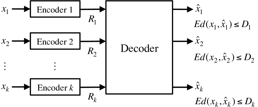
Figure 1: The $k$-encoder source coding problem.

Recently, it was shown in [10] that the Gaussian noise is the worst-case noise for general multi-hop multi-flow wireless networks. The main idea was to apply an OFDM-like scheme at all transmitters and receivers in the network in order to “mix” different noise realizations over time. This mixing, if performed over sufficiently long blocks, allows the Central Limit Theorem to kick in, effectively creating a new network where the additive noises are approximately Gaussian. This allows a coding scheme designed for a wireless network with Gaussian noise terms to achieve the same rates of reliable communication on a network with non-Gaussian noises.

In this paper, we show that similar ideas to the ones used in [10] can be used in the quadratic $k$-encoder source coding problem, if the source is not Gaussian. By having each encoder apply a DFT-based unitary linear transformation to its vector of source symbols, it is possible to create an approximately Gaussian source with the same covariance matrix. This allows us to prove that, for a given covariance matrix, the jointly Gaussian source is indeed the worst-case source for the $k$-encoder source coding problem. Moreover, this technique can be seen as a way of modifying codes designed for Gaussian sources so that they can be applied to non-Gaussian sources and still have a performance guarantee.

II Problem Setup and Main Result

We consider the $k$-encoder rate-distortion problem with a quadratic distortion measure. In this problem, $k$ encoders observe different components of a vector-valued i.i.d. sequence $\{(x_{1}[i],...,x_{k}[i])\}_{i=0}^{n-1}$. We assume that $(x_{1}[0],...,x_{k}[0])$ has an arbitrary distribution with zero mean and covariance matrix ${\bf K}$. Encoder $m$ maps ${\bf x}_{m}=(x_{m}[0],...,x_{m}[n-1])$ to an integer $f_{m}({\bf x}_{m})\in\{1,...,2^{nR_{m}}\}$, which is transmitted noiselessly to a central decoder. Given the $k$ integers $f_{m}({\bf x}_{m})$, $m=1,...,k$, the decoder uses decoding functions $g_{1},...,g_{m}$ in order to obtain estimates $(\hat{x}_{m}[0],...,\hat{x}_{m}[n-1])=g_{m}\left(f_{1}({\bf x}_{1}),...,f_{k}({\bf x}_{k})\right)$, for $m=1,...,k$. A code for the $k$-Encoder Rate-Distortion problem is comprised of a set of encoding and decoding functions $\left(f_{1},...,f_{m},g_{1},...,g_{k}\right)$ for a given blocklength $n$.

Definition 1.

Rate-distortion vector $(R_{1},...,R_{k},D_{1},...,D_{k})$ is achievable if, for some blocklength $n$, there exists a code $(f_{1},...,f_{m},g_{1},...,g_{m})$ for which

$$\tfrac{1}{n}E\left[\left\|{\bf x}_{m}-g_{m}(f_{1}({\bf x}_{1}),...,f_{k}({\bf x}_{k}))\right\|^{2}\right]\leq D_{m},$$ (1)

for $m=1,...,k$.

The following result establishes that the jointly Gaussian distribution is the worst-case source distribution among those with covariance matrix $\bf K$.

Theorem 1.

If rate-distortion vector $(R_{1},...,R_{k},D_{1},...,D_{k})$ is achievable when $(x_{1}[0],...,x_{k}[0])$ is jointly Gaussian with covariance matrix ${\bf K}$, then, for any $\epsilon>0$, rate-distortion vector $(R_{1}+\epsilon,...,R_{k}+\epsilon,D_{1}+\epsilon,...,D_{k}+\epsilon)$ is achievable when $(x_{1}[0],...,x_{k}[0])$ has any arbitrary distribution with covariance matrix ${\bf K}$.

III Proof of Main Result

In order to prove Theorem 1, we will need the following lemma, whose proof is in the Appendix.

Lemma 1.

Assume $(x_{1}[0],...,x_{k}[0])$ is jointly Gaussian. For any code $(f_{1},...,f_{k},g_{1},...,g_{k})$ that achieves rate-distortion vector $(R_{1},...,R_{k},D_{1},...,D_{k})$ and any $\epsilon,\epsilon^{\prime}>0$, one can find another code $(\tilde{f}_{1},...,\tilde{f}_{k},\tilde{g}_{1},...,\tilde{g}_{k})$ that achieves the rate-distortion vector $(R_{1}+\epsilon,...,R_{k}+\epsilon,D_{1}+\epsilon^{\prime},...,D_{k}+\epsilon^{\prime})$ for which the set of discontinuities of each $\tilde{f}_{m}$, $m=1,...,k$, has Lebesgue measure zero.

Proof of Theorem 1.

Suppose the rate-distortion vector $(R_{1},...,R_{k},D_{1},...,D_{k})$ is achievable in the case where $(x_{1}[0],...,x_{k}[0])$ is jointly Gaussian with covariance matrix ${\bf K}$. Fix $\epsilon>0$. From Lemma 1, we can assume that we have a code $(f_{1},...,f_{k},g_{1},...,g_{k})$ with blocklength $n$, which achieves rate-distortion vector $(R_{1}+\epsilon,...,R_{k}+\epsilon,D_{1}+\epsilon/2,...,D_{k}+\epsilon/2)$ if $(x_{1}[0],...,x_{k}[0])$ is jointly Gaussian, and such that the set of discontinuities of each $f_{m}$, $m=1,...,k$, has Lebesgue measure zero. We will then construct new encoding functions $\tilde{f}_{1},...,\tilde{f}_{k}$ with blocklength $nb$, for a large integer $b$, where $\tilde{f}_{m}$ is applied to the source sequence ${\bf x}_{m}=(x_{m}[0],...,x_{m}[nb-1])$, for $m=1,...,k$. The construction of these new encoding functions is illustrated in Figure 2.

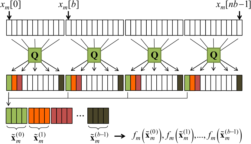
Figure 2: Illustration of the new encoding procedure for encoder $m$.

Encoder $m$ starts by applying a unitary ($2$-norm preserving) linear transformation ${\bf Q}$ (defined later) to each block of length $b$. The $n$ resulting blocks of length $b$ are then interleaved, generating $b$ length-$n$ vectors $\tilde{{\bf x}}_{m}^{(0)},...,\tilde{{\bf x}}_{m}^{(b-1)}$, as shown in Figure 2. The original encoding function $f_{m}$ (which takes as input a length-$n$ vector) is then individually applied to each $\tilde{{\bf x}}_{m}^{(i)}$, for $i=0,...,b-1$. This generates $b$ integers in $\{1,...,2^{n(R_{m}+\epsilon)}\}$ which can then be combined into a single integer from $\{1,...,2^{nb(R_{m}+\epsilon)}\}$ to produce the encoder output $\tilde{f}_{m}({\bf x}_{m})$.

At the decoder side, each $\tilde{f}_{m}({\bf x}_{m})$, for $m=1,...,k$, is first broken into the $b$ original integers from $\{1,...,2^{n(R_{m}+\epsilon)}\}$. Then, using the original decoding function $g_{m}$, the decoder obtains estimates of ${\bf\tilde{x}}_{m}^{(i)}$, for $i=0,...,b-1$, which can then be converted to an estimate of ${\bf x}_{m}$ by applying ${\bf Q}^{-1}$ $n$ times. This defines the new decoding functions $\tilde{g}_{m}$, $m=1,...,k$.

We define the unitary matrix ${\bf Q}$ by having the entry in the $(i+1)$th row and $(j+1)$th column be

$$Q{(i,j)}=\left\{\begin{array}[]{ll}1/\sqrt{b}&\text{if $i=0$}\\ \sqrt{2/b}\cos\left(\frac{2\pi j\ell}{b}\right)&\text{if $i=1,...,\frac{b}{2}-1$}\\ (-1)^{j}/\sqrt{b}&\text{if $i=\frac{b}{2}$}\\ \sqrt{2/b}\sin\left(\frac{2\pi j(\ell-b/2)}{b}\right)&\text{if $i=\frac{b}{2}+1,...,b-1$}\end{array}\right.$$

for $i,j\in\{0,...,b-1\}$. We point out that applying the linear transformation ${\bf Q}$ to a vector ${\bf x}$ can be seen as first taking the DFT of ${\bf x}$, then separating the real and imaginary parts of the resulting vector, and renormalizing them so that the resulting transformation is unitary. Checking that ${\bf Q}$ is a unitary transformation, i.e., that $\|{\bf Q}{\bf x}\|=\|{\bf x}\|$ for any ${\bf x}\in{\mathbb{R}}^{b}$, is straightforward and thus omitted.

Our next goal is to show that, by choosing $b$ large enough, we can make the distortion of this new code arbitrarily close to the distortion of the original code applied to the Gaussian source. We start by noticing that, since ${\bf Q}$ is a unitary linear transformation, the distortion of our new code can be written in terms of ${{\bf\tilde{x}}}_{m}^{(\ell)}$ for $\ell=0,...,b-1$ as

$$\frac{1}{b}\sum_{\ell=0}^{b-1}\frac{1}{n}\left\|{\bf\tilde{x}}_{m}^{(\ell)}-g_{m}\left(f_{1}({\bf\tilde{x}}_{1}^{(\ell)}),...,f_{k}({\bf\tilde{x}}_{k}^{(\ell)})\right)\right\|^{2}.$$

For each $b=1,2,...$, we will let

$$\ell_{b}=\arg\max_{0\leq\ell\leq b-1}E\left\|{\bf\tilde{x}}_{m}^{(\ell)}-g_{m}\left(f_{1}({\bf\tilde{x}}_{1}^{(\ell)}),...,f_{k}({\bf\tilde{x}}_{k}^{(\ell)})\right)\right\|^{2},$$

i.e., the $\ell_{b}$th length-$n$ block has the largest expected distortion. Note that $\left\{\left(\tilde{x}_{1}^{(\ell_{b})}[i],...,\tilde{x}_{k}^{(\ell_{b})}[i]\right)\right\}_{i=0}^{n-1}$ is an i.i.d. sequence of length-$k$ random vectors. We will show that it converges in distribution to a sequence of i.i.d. jointly Gaussian random vectors with covariance matrix ${\bf K}$, as $b\to\infty$. Clearly, it suffices to show that $\left(\tilde{x}_{1}^{(\ell_{b})}[0],...,\tilde{x}_{k}^{(\ell_{b})}[0]\right)$ converges in distribution to a jointly Gaussian random vector with covariance matrix ${\bf K}$, as $b\to\infty$. In order to use the Cramér-Wold Theorem, we fix an arbitrary vector $(t_{1},...,t_{k})\in{\mathbb{R}}^{k}$ and we notice that

$$\sum_{m=1}^{k}t_{m}\tilde{x}_{m}^{(\ell_{b})}[0] =\sum_{m=1}^{k}t_{m}\sum_{j=0}^{b-1}x_{m}[j]~{}Q(\ell_{b},j)$$

$$=\sum_{j=0}^{b-1}\left(\sum_{m=1}^{k}t_{m}x_{m}[j]\right)Q(\ell_{b},j).$$ (2)

To characterize the convergence in distribution of (2), we will need the following result.

Theorem 2 (Lindeberg’s Central Limit Theorem [11]).

Suppose that for each $b=1,2,...$, the random variables $Y_{b,1},Y_{b,2},...,Y_{b,b}$ are independent. In addition, suppose that, for all $b$ and $i\leq b$, $E[Y_{b,i}]=0$, and let

$$s_{b}^{2}=\sum_{i=1}^{b}E\left[Y_{b,i}^{2}\right].$$ (3)

Then, if for all $\varepsilon>0$, Lindeberg’s condition

$$\frac{1}{s_{b}^{2}}\sum_{i=1}^{b}E\left(Y_{b,i}^{2}\,{\mathds{1}}\left\{|Y_{b,i}|\geq\varepsilon s_{b}\right\}\right)\rightarrow 0\text{ as $b\rightarrow\infty$}$$ (4)

holds, we have that

$$\frac{\sum_{i=1}^{b}Y_{b,i}}{s_{b}}\stackrel{{\scriptstyle d}}{{\rightarrow}}{\mathcal{N}}(0,1).$$

To apply Lindeberg’s CLT, we will let, for $j=0,...,b-1$,

$$Y_{b,j+1}=\sqrt{b}\left(\sum_{m=1}^{k}t_{m}x_{m}[j]\right)Q(\ell_{b},j).$$

Then, if we let ${\bf K}_{u,v}$ be the entry in the $u$th row and $v$th column of ${\bf K}$, we have

$$s_{b}^{2} =\sum_{j=1}^{b}E\left[Y_{b,j}^{2}\right]=b\sum_{j=1}^{b}Q^{2}(\ell_{b},j-1)$$

$$\quad\quad\quad\times E\left(\sum_{m=1}^{k}t_{m}x_{m}[j-1]\right)^{2}$$

$$=b\sum_{1\leq u,v\leq k}t_{u}t_{v}{\bf K}_{u,v}\sum_{j=1}^{b}Q^{2}(\ell_{b},j-1)$$

$$=b\sum_{1\leq u,v\leq k}t_{u}t_{v}{\bf K}_{u,v},$$

regardless of the value of $\ell_{b}$. In order to verify Lindeberg’s condition, we define $\sigma^{2}=\sum_{1\leq u,v\leq k}t_{u}t_{v}{\bf K}_{u,v}$ and we let $U_{b,j}=Y_{b,j}^{2}\,{\mathds{1}}\left\{|Y_{b,j}|\geq\varepsilon s_{b}\right\}=Y_{b,j}^{2}\,{\mathds{1}}\left\{|Y_{b,j}|\geq\varepsilon\sigma\sqrt{b}\right\}$. Consider any sequence $j_{b}$, for $b=1,2,...$, such that $j_{b}\in\{1,...,b\}$, and any $\delta>0$. Then we have that

$$\Pr\left(U_{b,j_{b}}<\delta\right) \geq\Pr\left(|Y_{b,j_{b}}|<\varepsilon\sigma\sqrt{b}\right)$$

$$\geq\Pr\left(\left|\sum_{m=1}^{k}t_{m}x_{m}[j_{b}-1]\right|\sqrt{2}<\varepsilon\sigma\sqrt{b}\right)$$

$$=\Pr\left(\left|\sum_{m=1}^{k}t_{m}x_{m}[0]\right|<\varepsilon\sigma\sqrt{b/2}\right)\rightarrow 1,$$

as $b\rightarrow\infty$, which means that $U_{b,j_{b}}\stackrel{{\scriptstyle p}}{{\rightarrow}}0$ as $b\rightarrow\infty$. Moreover, we have that

$$\Pr\left(|U_{b,j_{b}}|\geq t\right) \leq\Pr\left[2\left(\sum_{m=1}^{k}t_{m}x_{m}[j_{b}-1]\right)^{2}\geq t\right]$$

$$=\Pr\left[2\left(\sum_{m=1}^{k}t_{m}x_{m}[0]\right)^{2}\geq t\right]$$

for $t>0$, and

$$E\left[2\left(\sum_{m=1}^{k}t_{m}x_{m}[0]\right)^{2}\right]=2\sigma^{2}<\infty,$$

and by the Dominated Convergence Theorem [11, pages 338-339], we have that $E[U_{b,j_{b}}]\rightarrow 0$ as $b\to\infty$. We conclude that

$$\frac{1}{s_{b}^{2}}\sum_{i=1}^{b}E\left(Y_{b,j}^{2}\,{\mathds{1}}\left\{|Y_{i}|\geq\varepsilon s_{b}\right\}\right) =\frac{1}{\sigma^{2}b}\sum_{j=1}^{b}E\left[U_{b,j}\right]$$

$$\leq\frac{1}{\sigma^{2}}\max_{1\leq j\leq b}E\left[U_{b,j}\right]\to 0,$$

as $b\to\infty$, and Lindeberg’s condition (4) is satisfied for any $\varepsilon>0$. Hence, from Theorem 2, we have that

$$\frac{\sum_{i=1}^{b}Y_{b,j}}{\sigma\sqrt{b}}\stackrel{{\scriptstyle d}}{{\rightarrow}}{\mathcal{N}}(0,1),$$

which implies, from (2), that

$$\sum_{m=1}^{k}t_{m}\tilde{x}_{m}^{(\ell_{b})}[0] =\sum_{j=0}^{b-1}\left(\sum_{m=1}^{k}t_{m}x_{m}[j]\right)Q(\ell_{b},j)$$

$$=\frac{\sum_{j=1}^{b}Y_{b,j}}{\sqrt{b}}\stackrel{{\scriptstyle d}}{{\rightarrow}}{\mathcal{N}}(0,\sigma^{2}).$$

Finally, since for a jointly Gaussian vector $(y_{1},...,y_{k})$ with mean zero and covariance matrix ${\bf K}$, we have $\sum_{m=1}^{k}t_{m}y_{m}\sim{\mathcal{N}}(0,\sigma^{2})$, we conclude, from the Cramér-Wold Theorem that $\left(\tilde{x}_{1}^{(\ell_{b})}[0],...,\tilde{x}_{k}^{(\ell_{b})}[0]\right)$ converges in distribution to a jointly Gaussian random vector with zero mean and covariance matrix ${\bf K}$, as $b\to\infty$.

Now, since the set of discontinuities of $f_{m}$, for $m=1,...,k$, has Lebesgue measure zero, it is easy to see that the mapping

$$\left\{{\bf\tilde{x}}_{m}^{(\ell)}\right\}_{m=1}^{k}\mapsto\left\|{\bf\tilde{x}}_{m}^{(\ell)}-g_{m}\left(f_{1}({\bf\tilde{x}}_{1}^{(\ell)}),...,f_{k}({\bf\tilde{x}}_{k}^{(\ell)})\right)\right\|^{2},$$

for $m=1,...,k$, must also have a set of discontinuities with Lebesgue measure zero. We conclude that

$$\left\|{\bf\tilde{x}}_{m}^{(\ell_{b})}-g_{m}\left(f_{1}({\bf\tilde{x}}_{1}^{(\ell_{b})}),...,f_{k}({\bf\tilde{x}}_{k}^{(\ell_{b})})\right)\right\|^{2}$$

$$\quad\quad\stackrel{{\scriptstyle d}}{{\to}}\left\|{\bf y}_{m}-g_{m}\left(f_{1}({\bf y}_{1}),...,f_{k}({\bf y}_{k})\right)\right\|^{2},$$

as $b\to\infty$, where ${\bf y}_{m}=(y_{m}[0],...,y_{m}[n-1])$, for $m=1,...,k$, and $\left\{\left(y_{1}[i],...,y_{k}[i]\right)\right\}_{i=0}^{n-1}$ is an i.i.d. sequence such that $(y_{1}[0],...,y_{k}[0])$ is jointly Gaussian with zero mean and covariance matrix ${\bf K}$. Moreover, we have that

$$\left\|{\bf\tilde{x}}_{m}^{(\ell_{b})}-g_{m}\left(f_{1}({\bf\tilde{x}}_{1}^{(\ell_{b})}),...,f_{k}({\bf\tilde{x}}_{k}^{(\ell_{b})})\right)\right\|^{2}$$

$$\quad\quad\leq 2\left\|{\bf\tilde{x}}_{m}^{(\ell_{b})}\right\|^{2}+2\left\|g_{m}\left(f_{1}({\bf\tilde{x}}_{1}^{(\ell_{b})}),...,f_{k}({\bf\tilde{x}}_{k}^{(\ell_{b})})\right)\right\|^{2}$$

$$\quad\quad\leq 2\left\|{\bf\tilde{x}}_{m}^{(\ell_{b})}\right\|^{2}+2\max_{c_{1},...,c_{k}}\left\|g_{m}(c_{1},...,c_{k})\right\|^{2},$$

and also that

$$E\left\|{\bf\tilde{x}}_{m}^{(\ell_{b})}\right\|^{2} =nE\left(\sum_{j=0}^{b-1}x_{m}[j]~{}Q(\ell_{b},j)\right)^{2}$$

$$=n{\bf K}_{m,m}\sum_{j=0}^{b-1}Q^{2}(\ell_{b},j)$$

$$=n{\bf K}_{m,m}<\infty.$$

Thus, from a variation of the Dominated Convergence Theorem (see Problem 16.4 in [11]), we conclude that, as $b\to\infty$,

$$E\left\|{\bf\tilde{x}}_{m}^{(\ell_{b})}-g_{m}\left(f_{1}({\bf\tilde{x}}_{1}^{(\ell_{b})}),...,f_{k}({\bf\tilde{x}}_{k}^{(\ell_{b})})\right)\right\|^{2}$$

$$\quad\to E\left\|{\bf y}_{m}-g_{m}\left(f_{1}({\bf y}_{1}),...,f_{k}({\bf y}_{k})\right)\right\|^{2}\leq n(D_{m}+\epsilon/2).$$

Therefore, we can choose $b$ sufficiently large so that

$$\frac{1}{n}E\left\|{\bf\tilde{x}}_{m}^{(\ell_{b})}-g_{m}\left(f_{1}({\bf\tilde{x}}_{1}^{(\ell_{b})}),...,f_{k}({\bf\tilde{x}}_{k}^{(\ell_{b})})\right)\right\|^{2}$$

$$\quad\quad\quad\quad\leq\frac{1}{n}E\left\|{\bf y}_{m}-g_{m}\left(f_{1}({\bf y}_{1}),...,f_{k}({\bf y}_{k})\right)\right\|^{2}+\epsilon/2$$

$$\quad\quad\quad\quad\leq D_{m}+\epsilon.$$

The expected distortion of our code $(\tilde{f}_{1},...,\tilde{f}_{k},\tilde{g}_{1},...,\tilde{g}_{k})$ (with blocklength $nb$) thus satisfies

$$\frac{1}{nb}\sum_{\ell=0}^{b-1}E\left\|{\bf\tilde{x}}_{m}^{(\ell)}-g_{m}\left(f_{1}({\bf\tilde{x}}_{1}^{(\ell)}),...,f_{k}({\bf\tilde{x}}_{k}^{(\ell)})\right)\right\|^{2}$$

$$\quad\quad\quad\quad\leq\frac{1}{n}E\left\|{\bf\tilde{x}}_{m}^{(\ell_{b})}-g_{m}\left(f_{1}({\bf\tilde{x}}_{1}^{(\ell_{b})}),...,f_{k}({\bf\tilde{x}}_{k}^{(\ell_{b})})\right)\right\|^{2}$$

$$\quad\quad\quad\quad\leq D_{m}+\epsilon,$$

for $m=1,...,k$. This concludes the proof of Theorem 1. ∎

Appendix A Appendix

Proof of Lemma 1.

Let $(x_{1}[0],...,x_{k}[0])$ be jointly Gaussian. If we assume that the rate-distortion vector $(R_{1},...,R_{k},D_{1},...,D_{k})$ is achievable, for some blocklength $n$, there exists a code $(f_{1},...,f_{m},g_{1},...,g_{m})$ for which (1) is satisfied for $m=1,...,k$. We follow the construction from [12] to build a code $(\tilde{f}_{1},...,\tilde{f}_{m},\tilde{g}_{1},...,\tilde{g}_{m})$ with the same blocklength $n$, which satisfies

$$\tfrac{1}{n}E\left\|{\bf x}_{m}-\tilde{g}_{m}(\tilde{f}_{1}({\bf x}_{1}),...,\tilde{f}_{k}({\bf x}_{k}))\right\|^{2}\leq D_{m}+\epsilon^{\prime}$$

for $m=1,...,k$.

Since our code can be repeated over multiple blocks of length $n$, we may assume that $n$ is large enough so that $2^{nR_{m}}+1\leq 2^{n(R_{m}+\epsilon)}$ for each $m$. Focus on encoder $f_{1}$, and let $B_{j}=f_{1}^{-1}(j)$, for $j\in\{1,...,2^{nR_{1}}\}$. Then, the $B_{j}$’s are a partition of ${\mathbb{R}}_{n}$. For each $j$, from Theorem 11.4 in [11], for any $\delta>0$, there exists a countable (in fact, finite) union of disjoint bounded rectangles $\tilde{B}_{j}$ such that $\Pr[{\bf x}_{1}\in B_{j}\vartriangle\tilde{B}_{j}]<\delta$. Then we define $\tilde{f}_{1}$ as

$$\tilde{f}_{1}({\bf x}_{1})=\left\{\begin{array}[]{ll}j&\text{if ${\bf x}\in\tilde{B}_{j}\setminus\bigcup_{i\neq j}\tilde{B}_{i}$}\\ 0&\text{otherwise.}\end{array}\right.$$

We create the encoders $\tilde{f}_{2},...,\tilde{f}_{k}$ in the same way. For $m=1,...,k$, our decoders will be

$$\tilde{g}_{m}(j_{1},...,j_{k})=\left\{\begin{array}[]{ll}g_{m}(j_{1},...,j_{k})&\text{if $j_{i}\neq 0$ for $i=1,...,k$}\\ 0&\text{otherwise.}\end{array}\right.$$

The new code is similar to the original one in the sense that, if we let $A$ be the event

$$\left\{g_{m}\left(f_{1}({\bf x}_{1}),...,f_{k}({\bf x}_{k})\right)\neq\tilde{g}_{m}\left(\tilde{f}_{1}({\bf x}_{1}),...,\tilde{f}_{k}({\bf x}_{k})\right)\right.$$

$$\hskip 56.9055pt\left.\text{ for some }m\in\{1,...,k\}\right\}$$

then, by the union bound,

$$\Pr\left[A\right]\leq\delta\sum_{m=1}^{k}2^{nR_{m}}.$$

It is clear that this new code has rates at most $R_{1}+\epsilon,...,R_{k}+\epsilon$. Following the derivation in [12], the distortion for decoder $g_{1}$ satisfies

$$E\left[\left\|{\bf x}_{1}-\tilde{g}_{1}\left(\tilde{f}_{1}({\bf x}_{1}),...,\tilde{f}_{k}({\bf x}_{k})\right)\right\|^{2}\right]$$

$$\leq E\left[\left\|{\bf x}_{1}-\tilde{g}_{1}\left(\tilde{f}_{1}({\bf x}_{1}),...,\tilde{f}_{k}({\bf x}_{k})\right)\right\|^{2}{\mathds{1}}_{A^{c}}\right]$$

$$\quad\quad+E\left[\left\|{\bf x}_{1}-\tilde{g}_{1}\left(\tilde{f}_{1}({\bf x}_{1}),...,\tilde{f}_{k}({\bf x}_{k})\right)\right\|^{2}\;{\mathds{1}}_{A}\right]$$

$$\stackrel{{\scriptstyle(i)}}{{\leq\;}}E\left[\left\|{\bf x}_{1}-g_{1}\left(f_{1}({\bf x}_{1}),...,f_{k}({\bf x}_{k})\right)\right\|^{2}\right]+M\sqrt{\delta}$$

$$\leq nD_{1}+M\sqrt{\delta},$$

where $(i$) follows by using Cauchy-Schwarz to obtain

$$E\left[\left\|{\bf x}_{1}-\tilde{g}_{1}\left(\tilde{f}_{1}({\bf x}_{1}),...,\tilde{f}_{k}({\bf x}_{k})\right)\right\|^{2}{\mathds{1}}_{A}\right]$$

$$\leq 2E\left[\left\|{\bf x}_{1}\right\|^{2}{\mathds{1}}_{A}\right]\ +2E\left[\left\|\tilde{g}_{1}\left(\tilde{f}_{1}({\bf x}_{1}),...,\tilde{f}_{k}({\bf x}_{k})\right)\right\|^{2}{\mathds{1}}_{A}\right]$$

$$\leq 2E\left[\left\|{\bf x}_{1}\right\|^{4}\right]^{1/2}E\left[{\mathds{1}}_{A}\right]^{1/2}$$

$$\quad\quad+2\max_{{\bf x}}\left\|\tilde{g}_{1}\left(\tilde{f}_{1}({\bf x}_{1}),...,\tilde{f}_{k}({\bf x}_{k})\right)\right\|^{2}E\left[{\mathds{1}}_{A}\right]^{1/2}$$

$$\leq\left(2E\left[\left\|{\bf x}_{1}\right\|^{4}\right]^{1/2}+2\max_{{\bf x}}\left\|\tilde{g}_{1}\left(\tilde{f}_{1}({\bf x}_{1}),...,\tilde{f}_{k}({\bf x}_{k})\right)\right\|^{2}\right)$$

$$\quad\quad\times\sqrt{\delta\sum_{m=1}^{k}2^{nR_{m}}}$$

$$=M\sqrt{\delta},$$

where $M$ is a finite number, independent of $\delta$. Therefore, we can choose $\delta>0$ sufficiently small so that $M\sqrt{\delta}\leq n\epsilon^{\prime}$, and the distortion of each decoder $g_{m}$ is at most $D_{m}+\epsilon^{\prime}$. Finally, we need to show that the set of discontinuities of each $\tilde{f}_{m}$ has measure zero. If we again focus on $\tilde{f}_{1}$, this function partitions ${\mathbb{R}}_{n}$ into $\hat{B}_{j}=\tilde{B}_{j}\setminus\cup_{i\neq j}\tilde{B}_{i}$ for $j=1,...,2^{nR_{1}}$ and $\hat{B}_{0}={\mathbb{R}}^{n}\setminus\cup_{j}\hat{B}_{j}$. Moreover, since the $\tilde{B}_{j}$’s were countable unions of disjoint bounded rectangles, and the class of bounded rectangles forms a semiring [11], the $\hat{B}_{j}$’s are also countable unions of disjoint bounded rectangles. Therefore, for a given $j$, we can write $\hat{B}_{j}=\cup_{i}S_{i}$, where the $S_{i}$’s are disjoint bounded rectangles. Moreover, we can also write $\hat{B}_{j}^{c}=\cup_{i}T_{i}$, where the $T_{i}$’s are disjoint bounded rectangles. Thus, we have

$$\partial\hat{B}_{j} =\partial\left(\cup_{i}S_{i}\right)={\mathbb{R}}^{n}-\left(\cup_{i}S_{i}\right)^{\circ}-\left(\cup_{i}T_{i}\right)^{\circ}$$

$$=\left(\cup_{i}S_{i}\right)\cup\left(\cup_{i}T_{i}\right)-\left(\cup_{i}S_{i}\right)^{\circ}-\left(\cup_{i}T_{i}\right)^{\circ}$$

$$\subseteq\left(\cup_{i}S_{i}\right)\cup\left(\cup_{i}T_{i}\right)-\left(\cup_{i}S_{i}^{\circ}\right)-\left(\cup_{i}T_{i}^{\circ}\right)$$

$$=\left(\cup_{i}\left(S_{i}-S_{i}^{\circ}\right)\right)\cup\left(\cup_{i}\left(T_{i}-T_{i}^{\circ}\right)\right)$$

$$\subseteq\left(\cup_{i}\partial S_{i}\right)\cup\left(\cup_{i}\partial T_{i}\right)$$

Since the boundary of a bounded rectangle clearly has Lebesgue measure zero, we have, for each $i$, $\lambda(\partial S_{i})=\lambda(\partial T_{i})=0$, and we conclude that

$$\lambda(\partial\hat{B}_{j})\leq\sum_{i}\lambda\left(\partial S_{i}\right)+\sum_{i}\lambda\left(\partial T_{i}\right)=0,$$

implying that the boundary of the partition of ${\mathbb{R}}_{n}$ induced by $\tilde{f}_{m}$ has Lebesgue measure zero. ∎

References

• [1] D. Slepian and J. Wolf. Noiseless coding of correlated information soruces. IEEE Trans. on Information Theory, 19:471–480, July 1973.
• [2] R. Ahlswede and J. Körner. Source coding with side information and a converse for degraded broadcast channels. IEEE Trans. on Information Theory, 21:629–637, Nov. 1975.
• [3] A. Wyner. On source coding with side information at the decoder. IEEE Trans. on Information Theory, 21:294–300, May 1975.
• [4] A. Wyner and J. Ziv. The rate-distortion function for source coding with side information at the decoder. IEEE Trans. on Information Theory, 22:1–10, Jan. 1976.
• [5] T. Berger and R. Yeung. Multiterminal source encoding with one distortion criterion. IEEE Trans. on Information Theory, 35:228–236, Mar. 1989.
• [6] A.B. Wagner, S. Tavildar, and P. Viswanath. Rate region of the quadratic Gaussian two-encoder source-coding problem. IEEE Transactions on Information Theory, 54(5):1938–1961, May 2008.
• [7] R. Gallager. Information Theory and Reliable Communication. Wiley, New York, 1968.
• [8] T. Berger. Multiterminal source coding. In G. Longo, editor, The Information Theory Approach to Communications, CISM Courses and Lectures, pages 171–231. Springer-Verlag, New York, 1978.
• [9] S.-Y. Tung. Multiterminal Source Coding. PhD thesis, Cornell University, Ithaca, NY, 1978.
• [10] I. Shomorony and A. S. Avestimehr. Worst-case additive noise in wireless networks. in arXiv:cs.IT/1202.2687, 2012.
• [11] P. Billingsley. Probability and Measure. Wiley Series in Probability and Mathematical Statistics. John Wiley & Sons, 3rd edition, 1995.
• [12] J. Chen and A. B. Wagner. A semicontinuity theorem and its application to network source coding. Proc. of IEEE ISIT 2008, Toronto, Canada, pages 429–433, 2008.