Equivalence between microcanonical methods for lattice models

Abstract

The development of reliable methods for estimating microcanonical averages constitutes an important issue in statistical mechanics. One possibility consists of calculating a given microcanonical quantity by means of typical relations in the grand-canonical ensemble. But given that distinct ensembles are equivalent only at the thermodynamic limit, a natural question is if finite size effects would prevent such procedure. In this work we investigate thoroughly this query in different systems yielding first and second order phase transitions. Our study is carried out from the direct comparison with the thermodynamic relation $(\frac{\partial s}{\partial e})$, where the entropy is obtained from the density of states. A systematic analysis for finite sizes is undertaken. We find that, although results become inequivalent for extreme low system sizes, the equivalence holds true for rather small $L$’s. Therefore direct, simple (when compared with other well established approaches) and very precise microcanonical quantities can be obtained from the proposed method.

PACS numbers: 05.10.Ln, 05.20.Gg, 05.50.+q

I Introduction

The development of efficient Monte Carlo (MC) methods constitutes a key problem in statistical mechanics. Typically, numerical simulations are performed by one-flip algorithms that generate a grand-canonical ensemble, in which intensive quantities are held fixed landaubook . However, in some cases, a different ensemble would be more appropriate. For example, strong first-order phase transitions become extremely hard to simulate by one-flip grand-canonical schemes: the presence of different phases separated by large free-energy barriers makes the system to be trapped into metastable states at the phase coexistence, even for small system sizes. Although different grand-canonical procedures have been proposed bouabci ; berg ; fioreprl , the microcanonical ensemble is also an appropriate way to circumvent these problems. In this case, the simulation is carried out for fixed energies and intensive thermodynamic quantities are treated as external variables, hence avoiding large entropic barriers.

Different microcanonical schemes have been proposed in the last years. Entropic sampling lee , broad histogram method pmc and the Wang-Landau (WL) method wang are some examples of procedures in which the density of states (DOS) is estimated numerically. Other microcanonical approaches, not requiring the knowledge of the DOS, have also been developed. In such cases, the temperature and other intensive quantities are obtained from auxiliary relations. For example, Creutz creutz has generated a microcanonical ensemble by assuming a canonical distribution of the energies carried by a “demon”, where the total energy is not strictly conserved, but it fluctuates above a constant lower bound. More recently, Martin-Mayor mayor proposed a method where the temperature is obtained from an ensemble of fixed energy (including the kinetic energy). The temperature is calculated from the fluctuations of the spin part.

To analyze the discontinuous transitions in the Blume-Emery-Griffiths (BEG) BEGMODEL and asymmetric Ising models wang2 , it has been employed a “trick” fiore6 , where intensive quantities are calculated through expressions originally derived in the grand-canonical ensemble. Although the equivalence is granted in the thermodynamic limit, Gibbs ensembles may be inequivalent for finite systems, including short range interactions at the phase coexistence gross . Therefore, in order to the protocol can be extended to more general situations, one should test under what conditions the finite size effects hinder the equivalence between methods. In other words, it should be verified that intensive quantity as a matter of fact correspond to the genuine microcanonical temperature (obtained from the derivation of entropy with respect to the energy).

The first goal of this paper is then to answer the above query. For so, different aspects of the method will be exemplified by means of distinct lattice systems yielding first and second-order phase transitions. We first address the Ising model, for which the DOS are known exactly beale . Then we consider as next examples the Blume-Capel (BC) and the Potts models. Although they do not present exact DOS, we are going to compare with the very efficient WL sampling as a benchmark. The BC model is an interesting case, since its DOS has been obtained by performing a random walk in the space of two parameters (in similarity to several lattice models presenting distinct particle interactions) claudio ; wang2 . We intend to verify if the calculation of the temperature will be changed by different restrictions in the random walk (as performed in Ref. claudio ).

The Potts models is also a very interesting test. Unlike the previous cases, its discontinuous transitions (yielding for $q>4$) presents a genuine microcanonical feature, the existence of a loop lee ; mayor ; komura . Thus, it is important to verify if our approach not only reproduces this remarkable signature but also is equivalent to the $(\frac{\partial s}{\partial e})$. In addition, we are also exploiting the interesting $q=4$ case, that although yielding a continuous transitions, it possesses distinct behaviors including logarithmic scaling corrections mayor ; fernandez ; sokal and a double peak probability distribution fukugita . As it will be shown further, the methods becomes equivalent in all above models for relatively small system sizes $L$. The equivalence includes not only the temperatures but also all extrapolated thermodynamic limit points. However, for extreme small $L$’s, the results do not agree and thus the intensive quantity can not be recognized as the thermodynamic temperature. We will present a detailed analysis showing how the methods converge when $L$ increases.

A second contribution here is to exploit the advantages. Besides its low computational cost, it does not require criterion for achieving convergence of results. Other immediate advantage is that intensive quantities are evaluated directly from standard numerical simulations and become more precise as the system size increases. In addition, the method is very easily extended for other lattice models.

This paper is organized as follows: In Sec. II we review the methods for calculating the temperature. In Sec. III we show the numerical results for the models and in Sec. IV we present our conclusions.

II Microcanonical Temperature

For a given system size $L$ and energy per site $e=E/V$ (where $V=L^{d}$ and $d$ is the dimension), the inverse of microcanonical temperature $\beta_{L}$ is obtained through the expression

$$\beta_{L}=(\frac{\partial s}{\partial e})_{L},$$ (1)

where $s=s(e,L)=\frac{k_{B}}{L^{d}}\ln\Omega(E,L)$ is the entropy per site and $\beta_{L}=1/k_{B}T_{L}$. The quantity $\Omega(E,L)$ denotes the DOS for given $E$ and $L$. For the Ising model, the $\Omega(E,L)$ is known exactly beale . For the other models, we shall estimate $\Omega(E,L)$ using the WL sampling wang .

The WL sampling is a powerful technique to calculate $\Omega(E,L)$ by carrying out a random walk in energy space with an acceptance probability proportional to $1/\Omega(E,L)$, i.e.,

$$P(E_{i}\rightarrow E_{j})=\min\left[\frac{\Omega(E_{i},L)}{\Omega(E_{j},L)},1\right],$$ (2)

where $E_{i}$ and $E_{j}$ are the energies of the current and a possible new configuration, respectively. For each new accepted configuration an energy histogram $H(E)$ is accumulated.

During the random walk, whenever a move to a configuration with energy $E$ is accepted, $\Omega(E,L)$ is updated by multiplying it by a “modification factor” $f>1$ that accelerates the diffusion of the random walk, and an unit is added to the histogram $H(E)$. The initial choice of $f$ is $f_{0}=e=2.71828\dots$. $\Omega(E,L)$ is multiplied by $f$ until the accumulated histogram $H(E)$ becomes flat. We then reduce $f$ by setting $f\rightarrow\sqrt{f}$, and resetting $H(E)=0$ for all energy values. The simulation converges to the true value of $\Omega(E,L)$ when $f$ approximates to the unit. In particular, in this work we use the improved Wang-Landau sampling proposed by Cunha-Netto et al. cunha . Their approach use adaptive energy windows to eliminate border effects that affect the density of states mainly of q-states Potts model, which is our case here. In our simulations the criterion of flatness was taken as each value of the histogram reaching at least $80$% of the mean value $\langle H(E)\rangle$ for the BC model and $90$% for the Potts model. The histograms are generally checked after each $10000$ MC steps. Here we performed $10$ different runs for the same $L$ with different initial seeds in order to reduce statistical fluctuations. For the BC model, the DOS is obtained by performing a random walk for two parameters $E$ and $E_{2}$ ($E_{2}=\sum_{i}\sigma_{i}^{2}$). An immediate advantage of the WL is that a single run gives the DOS for the whole range of energy, which provides the calculation of canonical averages for any temperature.

Now, following Ref. fiore6 we proceed to obtain the temperature $T$ with respect to the microcanonical ensemble. The method consists in writing down the probabilities of different microscopic configurations in the grand-canonical ensemble and further resorting the equivalence of ensembles.

The probability distribution $P(\sigma)$ of a microscopic configuration $\sigma=(\sigma_{1},\sigma_{2},...,\sigma_{V})$ in the grand-canonical ensemble is given by $P(\sigma)=\exp\{-\beta{\cal H}(\sigma)\}/\Xi$, with Hamiltonian ${\cal H}(\sigma)$ reading

$${\cal H(\sigma)}=-J\sum_{(i,j)}\sigma_{i}\sigma_{j},$$ (3)

for the Ising model and

$${\cal H(\sigma)}=-J\sum_{(i,j)}\sigma_{i}\sigma_{j}+\Delta\sum_{i}\sigma_{i}^{2},$$ (4)

for the BC model and

$${\cal H(\sigma)}=-J\sum_{(i,j)}\delta_{\sigma_{i},\sigma_{j}},$$ (5)

for the Potts model. Parameters $J$ and $\Delta$ are the energy between two nearest-neighbor spins and the crystalline field, respectively. The spin variable $\sigma$ takes the values $-1$ or $+1$ for the Ising model, $-1,0$ or $+1$ for the Blume-Capel and $0,1,...,q-1$, for the Potts model. In all cases, the summations are restricted over nearest neighbor sites.

By considering the transition $-1\leftrightarrow 1$ for Ising and BC models and denoting $\sigma^{k}$ by a microscopic configuration which differs from $\sigma$ only by the value of the spin at the site $k$, that is, $\sigma^{k}=(\sigma_{1},\sigma_{2},...,-\sigma_{k},..,\sigma_{V})$, the ratio between $P(\sigma)$ and $P(\sigma^{k})$ in the grand-canonical ensemble is given by

$$\frac{P(\sigma)}{P(\sigma^{k})}=\exp\{2\beta\sigma_{k}[\phi_{k}(\sigma)]\},$$ (6)

where

$$\phi_{k}(\sigma)=J\sum_{\delta}\sigma_{k+\delta},$$ (7)

whose summation is performed over $\delta$ nearest neighbor sites. If the average of an arbitrary state function in the grand-canonical ensemble is given by $\langle\ f(\sigma)\rangle_{gc}=\sum_{\sigma}f(\sigma)P(\sigma)$, from Eq. (6) we have that

$$\langle f(\sigma)\rangle_{gc}=\langle f(\sigma^{k})\exp\{2\beta\sigma_{k}[\phi_{k}(\sigma)]\}\rangle_{gc}.$$ (8)

By taking Eq. (8) for $f(\sigma)$ given by $f(\sigma)=\delta(\sigma_{k},+1)\delta(\phi_{k}(\sigma),{\bar{E}})$, we have that

$$e^{-2\beta{\bar{E}}}=\frac{\langle\delta(\sigma_{k},-1)\delta(\phi_{k}(\sigma),{\bar{E}})\rangle_{gc}}{\langle\delta(\sigma_{k},+1)\delta(\phi_{k}(\sigma),{\bar{E}})\rangle_{gc}},$$ (9)

where ${\bar{E}}$ denotes one of all possible values of $\phi_{k}(\sigma)$. In the microcanonical ensemble, the energy per site $e=E/V$ is held fixed. Assuming the equivalence between the grand-canonical and microcanonical ensembles, we get the following expression

$$e^{-2\beta{\bar{E}}}=\frac{\langle\delta(\sigma_{k},-1)\delta(\phi_{k}(\sigma),{\bar{E}})\rangle_{mc}}{\langle\delta(\sigma_{k},+1)\delta(\phi_{k}(\sigma),{\bar{E}})\rangle_{mc}},$$ (10)

which allows us to obtain the temperature $T$ with respect to the microcanonical ensemble. A similar procedure can be performed for the Potts model. By choosing two particular states $k^{*}$ and $k^{**}$ (ranging from $0$ to $q-1$) with respective transition $k^{*}\leftrightarrow k^{**}$ and the state function $h(\sigma)=\delta(\sigma_{k},k^{*})\delta(\phi_{k}(\sigma),{\bar{E}})$ we have, by appealing to the equivalence of ensembles, that

$$e^{-\beta{\bar{E}}}=\frac{\langle\delta(\sigma_{k},k^{*})\delta(\phi_{k}(\sigma),{\bar{E}})\rangle_{mc}}{\langle\delta(\sigma_{k},k^{**})\delta(\phi_{k}(\sigma),{\bar{E}})\rangle_{mc}},$$ (11)

where $\phi_{k}(\sigma)$ is given by $\phi_{k}(\sigma)=J\sum_{\delta}(\delta_{k^{**},\sigma_{k+\delta}}-\delta_{k^{*},\sigma_{k+\delta}})$. Since the above formulae does not specify the dynamics, they are valid for different classes of microcanonical algorithms.

III Numerical Results

Numerical simulations have been performed in a square lattice with $L^{2}$ sites. The microcanonical dynamics is composed of two parts. In the first part, a given site of the lattice is randomly chosen and its spin is changed to one of its all possible values. In the second part, two sites of the lattice, also randomly chosen, have theirs spins interchanged. The above dynamics are accepted only if the total energy remains unchanged. It is worth mentioning that the actual MC algorithm is quite different from those studied in Refs. fiore6 , where both energy and magnetization are strictly conserved. Here the particle moves are accepted only when the total energy does not change. The number of species (spins) is not necessarily conserved.

By applying the logarithm on both sides of Eq. (10), we get the following expression (written in units of $J$ and $k_{B}$)

$$\ln R_{n}=-\frac{2n}{T},$$ (12)

where the right-hand of Eq. (10) was written as $R_{n}$. The possible values of the quantity ${\bar{E}}=\phi_{k}(\sigma)=J\sum_{\delta}\sigma_{k+\delta}$ are given by $nJ$, where $n$ takes the values $n=-4,-2,0,2,4$, for the Ising model and $n=-4,-3,...,3,4$, for the BC model. Thus, from the above, by calculating $\ln R_{n}$ numerically for all possible values of $\phi_{k}(\sigma)$, the temperature is extracted from the inverse of the slope of Eq. (12). A similar procedure is done for the Potts model, where we have

$$\ln R_{n}=-\frac{n}{T},$$ (13)

where $n$ assumes the values $-4,-3,...,3,4$ for all values of $q$.

In the first analysis, we study the validity of Eqs. (12) and (13) for different $L$, as showed in Fig. 1$(a)$ and $(b)$ for the Ising model. Continuous lines and symbols denote standard and present results, respectively and temperatures calculated for $L=4$ are exact in both cases. Comparison between intensive quantities show that they are slightly different for the smallest $L$’s ($L=4$ and $L=6$). Inspection of part $(b)$ reveals us that in these cases, the quantity $\ln R_{n}$ is not linear in $n$, and hence Eq. (12) does not hold. The non validity of Eq. (12) for extreme small $L$ is exemplified by evaluating the numerator and denominator of Eq. (10) for $e=-1.25$ and $L=4$. Since the number of configurations is small, both quantities are zero for $n=0$, whereas for $n=4$ ($n=-4$) the numerator (denominator) is null. By increasing $L$ the number of configurations becomes large in such a way that the linear dependence between $\ln R_{n}$ and $n$ is achieved. Only in this regime we can evaluate $T$ from Eq. (12). In practice, estimates become equivalent for rather small system sizes. For example, for the Ising model the difference between estimates is in the third decimal level for $L=8$.

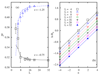
Figure 1: Inverse of temperature $\beta_{L}$ versus $L$ for different $e$’s for the Ising model. Symbols and continuous lines denote the estimates obtained from the present approach and the exact DOS, respectively. In $(b)$ we have a mono-log plot of the quantity $R_{n}$ versus $n$ for different $L$ and $e=-0.75$. Curves have been shifted in order to avoid overlapping and continuous lines have been used for better visualization of slopes.

Similar conclusions are verified for the other models, as exemplified in Fig. 2$(a)$ and $(b)$ for the $q=10$ Potts model. As in the Ising model, Eq. (13) is not hold for small $L$’s (exemplified in part ($b$) for $e=-1.25$), which becomes equivalent to $(\frac{\partial s}{\partial e})_{L}$ for larger (but still rather small) $L$’s.

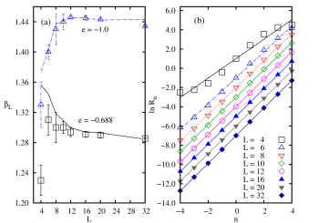
Figure 2: Inverse of temperature $\beta_{L}$ versus $L$ for different $e$’s for the $q=10$ Potts model. Symbols and continuous lines denote the estimates obtained from the present approach and the exact DOS, respectively. In $(b)$ we have a mono-log plot of the quantity $R_{n}$ versus $n$ for different $L$ and $e=-1.25$. Curves have been shifted in order to avoid overlapping and continuous lines have been used for better visualization of slopes.

It is worth remarking that due to the small number of configurations and the discretization of energy, both procedures are not precise in the limit of extreme low energies.

Once established the regime of convergence of methods, we extend the previous analysis for the whole range of energy. In Fig. 3 $(c)$, we plot the $\ln R_{n}$ as function of $n$ for several values of $E$ and $L=10$. Note that all curves are linear and cross at $(0,0)$, which gives $H=0$ for all energies and temperatures, in consistency with results by Beale beale , where the DOS was enumerated for $H=0$. In Fig. 3$(a)$ we plot $\beta_{L}$ versus the total energy $E$ for different $L$. In order to avoid data overlapping we choose to plot $E$ instead of $e=E/V$. The results for the Ising model show an excellent agreement between estimates of $\beta_{L}$ for all system sizes (part $(b)$).

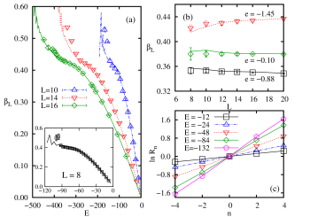
Figure 3: Inverse of temperature $\beta_{L}$ versus total energy $E$ for the Ising model and different system sizes $L$. Symbols and continuous lines (for $(a)$ and $(b)$) denote the estimates obtained from the present approach and the exact DOS, respectively. Inset shows the convergence of methods already achieved for $L=8$. In $(b)$ we have the $\beta_{L}$ versus $L$ for some values of $e=E/V$. In $(c)$ we have a mono-log plot of the quantity $R_{n}$ versus $n$ for $L=10$ and different values of $E$. Slopes of straight lines give $\beta_{L}$. In this case, continuous lines have been used for better visualization of slopes.

In addition, we have also compared (not shown) both schemes at the ferromagnetic-paramagnetic second-order phase transition. The pseudo-critical temperature $\beta_{L}^{*}$ may be estimated by the peak in the specific heat $C$ (obtained from the energy numerical differentiation). The deviation between $\beta_{L}^{*}$ and its asymptotic value $\beta_{c}=\frac{1}{2}\ln(1+\sqrt{2})$ (obtained here) agrees very well with exact estimates by Beale beale .

Further, we extend the previous analysis to the Blume-Capel model. In similarity with the WL model claudio , numerical simulations were performed for fixed $E=\sum_{(i,j)}\sigma_{i}\sigma_{j}$ and $E_{2}=\sum_{i}\sigma_{i}^{2}$. In practice, $E_{2}$ fixed implies that the number of spins $0$ is conserved. The one-flip part is restricted to only spins $\pm 1$. In Fig. 4$(a)$ we plot $\beta_{L}$ versus $E$ for different $E_{2}$, whereas in the graph $(b)$, we analyze the dependence of $\beta_{L}$ on $E_{2}$ for $E$ fixed. The dependence on $L$ is also showed in Fig. 4$(c)$. Note again a very good agreement between both approaches, even for small system sizes, supporting once more the equivalence between Eqs. (1) and (10).

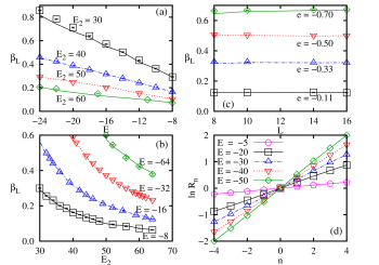
Figure 4: In $(a)$ and $(b)$ we plot the inverse of temperature $\beta_{L}$ as a function of $E$ ($E_{2}$) for the BC model with $E_{2}$ ($E$) fixed and $L=8$. Symbols and continuous lines denote estimates obtained from the present approach and from Wang-Landau method, respectively. In $(c)$ we show the dependence of $\beta_{L}$ on $L$ for different values of $e$ and $e_{2}=2/3$. In $(d)$ we plot $\ln R_{n}$ versus $n$ for $E$ for $e_{2}=2/3$ and $L=10$. Slopes of straight lines give $\beta_{L}$. In this case, continuous lines have been used for better visualization of slopes.

Now we take the Potts model in kind. As in the Ising and BC models, it also presents ferromagnetic-paramagnetic phase transitions, exactly located at $\beta_{0}=\ln(1+\sqrt{q})$. For $q\leq 4$, it is second-order which becomes first-order for $q>4$. The case $q=4$ presents remarkable features, including logarithmic scaling corrections mayor ; fernandez ; sokal and a double peak probability distribution fukugita , hence an interesting case to be considered. In Figs. 5$(a)$ and $(b)$ we evaluated $\beta_{L}$ for different energies and system sizes (relative small $L$’s but sufficient large to imply the validity of Eq. (13)). As in the previous examples, we have also found an excellent agreement between estimates obtained from microcanonical procedures. In the inset of Fig. 5$(a)$ we plot the pseudo-critical temperature $\beta_{L}^{*}$, obtained from the peak in the specific heat $C$. For $q=4$, the deviation of $\beta_{L}^{*}$ from its asymptotic value $\beta_{c}$ decays as $y\equiv\frac{(\ln L)^{3/4}}{L^{3/2}}$ fernandez ; sokal , where we found (by using this scaling law) the estimate $\beta_{c}=1.0982(4)$, in excellent agreement with the exact value $\beta_{c}=\ln(1+\sqrt{q})=1.0986123...$.

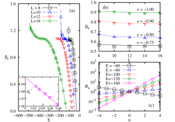
Figure 5: In $(a)$, we plot the inverse of temperature $\beta_{L}$ versus $E$ for several $L$ in the $q=4$ Potts model. Symbols and continuous lines denote estimates obtained from present approach and WL, respectively. In $(b)$ we plot the dependence of $\beta_{L}$ on $L$ for different values of $e$. In $(c)$ we plot the $\ln R_{n}$ versus $n$ for different energies and $L=10$. Slopes of straight lines give $\beta_{L}$. In this case, continuous lines have been considered for better visualization of slopes. In the inset we plot the inverse of the temperature $\beta_{L}^{*}$ in which specific heat presents a maximum versus $y\equiv\frac{(\ln L)^{3/4}}{L^{3/2}}$. The straight line has linear coefficient $\beta_{c}=1.0982(4)$.

In the last analysis, we evaluated the microcanonical temperature for the $q=10$ and $q=20$ states Potts model. These are also very interesting cases because, in contrast to all previous ones, they possesses discontinuous transitions characterized by a S-like structure, a “loop” komura , hence ideal examples for illustrating the correctness of the present approach. Loops for finite systems in the microcanonical ensemble are due to interfacial effects, in which the surface tension behaves as $1/L$ gross ; komura ; janke . In contrast, systems simulated in the grand-canonical ensemble do not present loops. In Fig. 6 we show the validity of Eq. (11) by plotting $\beta_{L}$ versus $e$ for $q=10$ (part $(a)$) and $q=20$ (part $(b)$) for $L=20$. As in all previous cases, we also have a good agreement between the temperatures, for both values of $q$. However, in contrast with our results, estimates obtained from the WL method presents large fluctuations, even using the adaptive windows improvement, taking the flatness criterion of 90$\%$ for the convergence of $H(E)$ and evaluating the mean DOS over 10 different seeds. On the other hand, our estimates become more precise as $L$ increases. For smaller system sizes they are less accurate (already taking the $L$ for which methods are equivalent), despite the accordance with estimates from the WL method. This can be understood in the following: Since the number of configurations for fixed $E$ is very large and the right side of Eq. (11) is evaluated from only two possible spins, averages become less precise for small $L$. By increasing $L$, the number of sites with above chosen spins are larger and therefore, the averages becomes more precise. This is an interesting point, since on the contrary to the WL, under the present approach $\beta_{L}$ becomes more precise by increasing $L$. In the inset of each figure, we plot the dependence of the minimum $\beta_{L}^{*}$ on $L^{-1}$, where the straight line have linear coefficients $\beta_{0}=1.4267(7)$ and $\beta_{0}=1.702(2)$, which agrees very well with the exact value $\beta_{0}=\ln(1+\sqrt{10})=1.42606...$ and $\beta_{0}=\ln(1+\sqrt{20})=1.699669...$.

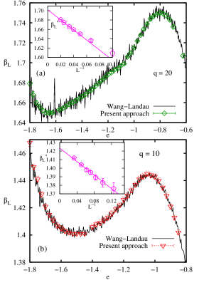
Figure 6: Inverse of temperature $\beta_{L}$ versus $e$ for the $q=10$ Potts model for $L=16$ (top) and $L=20$ (bottom). Symbols and continuous lines correspond to the estimates obtained from the present approach and WL, respectively. In the inset, we plot the dependence of the minimum $\beta_{L}^{*}$ versus $L^{-1}$, respectively. The straight line has linear coefficient $\beta_{0}=1.4267(7)$.

IV Conclusions

In this paper we have clarified the fundamental issue of a method proposed at Ref. fiore6 which uses a grand-canonical relationship for calculating microcanonical quantities. The study was carried out from the direct comparison with the standard definition of microcanonical temperature. A detailed analysis for three different lattice models yielding first and second-order phase transitions sizes was undertaken. Our results show that although methods are not equivalent for extreme small system sizes, they converge for relative small $L$’s (in practice, our definition becomes equivalent to $(\frac{\partial s}{\partial e})_{L}$ for $L=8$). Not only the estimates for finite systems were found to be equivalent, but also the thermodynamic limit transition points. The further contribution exploited its advantages. Besides the generality and easy implementation, thermodynamic quantities are precisely evaluated from rather short simulations. Other advantages of the method concerns its low computational cost and not requiring a criterion for achieving convergence of results. Once the equivalence has been verified in distinct situations, we believe that the present approach may offer a rather cheap method for simulating more complex systems, such as lattice models with continuous variables domany , spin-glasses and polymer systems landaubook . This will be the subject of ongoing work.

References

- (1) D. P. Landau and K. Binder, A Guide to Monte Carlo Simulation in Statistical Physics (Cambridge University Press, Cambridge, 2005).
- (2) M. B. Bouabci and C. E. I. Carneiro, Phys. Rev. B 54, 359 (1996); C. E. Fiore and C. E. I. Carneiro, Phys. Rev. E 76, 021118 (2007).
- (3) B. A. Berg and T. Neuhaus, Phys. Lett. B 267, 249 (1991); ibid, Phys. Rev. Lett. 68, 9 (1992).
- (4) C. E. Fiore and M. G. E. da Luz, Phys. Rev. Lett. 107, 230601 (2011).
- (5) J. Lee, Phys. Rev. Lett. 71, 211 (1993).
- (6) P. M. C. de Oliveira, Braz. J. Phys. 30, 195 (2000).
- (7) F. Wang and D. P. Landau, Phys. Rev. Lett. 86, 2050 (2001); Phys. Rev. E 64, 056101 (2001).
- (8) M. Creutz, Phys. Rev. Lett. 50, 1411 (1983).
- (9) V. Martin-Mayor, Phys. Rev. Lett. 98 137207 (2007).
- (10) M. Blume, V. J. Emery, and R. B. Griffiths, Phys. Rev. A 4, 1071 (1971); W. Hoston and A. N. Berker, Phys. Rev. Lett. 67, 1027 (1991).
- (11) S. Tsai, F. Wang and D. P. Landau, Phys. Rev. E 75, 061108 (2007).
- (12) C. E. Fiore, V. B. Henriques and M. J. de Oliveira, J. Chem. Phys. 125, 164509 (2006); C. E. Fiore and M. J. de Oliveira, Comp. Phys. Comm. 180, 1434 (2009).
- (13) D. H. E. Gross, Microcanical Thermodynamics, Lecture Notes in Physics, vol. 66, World Scientific, 2001; D. H. E. Gross, A. Ecker and X. Z. Zhang, arXiv:cond-mat/9607150v1.
- (14) P. D. Beale, Phys. Rev. Lett. 76, 78 (1996).
- (15) C. J. Silva, A. A. Caparica and J. A. Plascak, Phys. Rev. E 73, 036702 (2006).
- (16) See for example, Y. Komura and Y. Okabe, Phys. Rev. E 85, 010102(R) (2012).
- (17) L. A. Fernandez, A. Gordillo-Guerrero, V. Martin-Mayor and J. J. Ruiz-Lorenzo, Phys. Rev. E. 80, 051105 (2009).
- (18) J. Salas and A. D. Sokal, J. Stat. Phys. 88, 567 (1997).
- (19) M. Fukugita, H. Mino, M. Okawa, and A. Ukawa, J. Phys. A 23, L561 (1990).
- (20) A. G. Cunha Netto, A. A. Caparica, Shan-Ho Tsai, R. Dickman and D. P. Landau, Phys. Rev. E 78, 055701(R) (2008).
- (21) W. Janke, Nuc. Phys. B (Proc. Suppl.) 63A-C, 631 (1998).
- (22) See for example, E. Domany, M. Schick and R. H. Swendsen, Phys. Rev. Lett. 52, 1535 (1984).