Numerical investigation of the Bautin bifurcation in a delay differential equation modeling leukemia

Abstract

In a previous work we investigated the existence of Hopf degenerate bifurcation points for a differential delay equation modeling leukemia and we actually found Hopf points of codimension two for the considered problem. If around such a point we vary two parameters (the considered problem has five parameters), then a Bautin bifurcation should occur. In this work we chose a Hopf point of codimension two for the considered problem and perform numerical integration for parameters chosen in a neighborhood of the bifurcation point parameters. The results show that, indeed, we have a Bautin bifurcation in the chosen point.
Acknowledgement. Work partially supported by Grant 11/05.06.2009 within the framework of the Russian Foundation for Basic Research - Romanian Academy collaboration.
Keywords: delay differential equations, stability, Hopf bifurcation, Bautin bifurcation.
AMS MSC 2010: 37C75, 65L03, 37G05, 37G15.

1 Introduction

The considered equation was taken from [9], [10]

$$\dot{x}(t)=-\left[\frac{\beta_{0}}{1+x(t)^{n}}+\delta\right]x(t)+k\frac{\beta_{0}x(t-r)}{1+x(t-r)^{n}},$$ (1)

and represents part of a model of periodic chronic myelogenous leukemia. The initial model consists of two delay equations, one for the density of proliferating cells, $P$, and one for the density of so-called ”resting” cells, $N$. The latter equation is independent, hence it can be studied independently (see [9], [10]). Equation (1) is this second equation, with the unknown $N$ made dimensionless by dividing it by a quantity with the same dimension. The parameters $\beta_{0},\,n,\,\delta,\,k,\,r$ are positive real numbers. We do not insist here on their physical significance since this is largely presented in [9], [10]. Parameter $k$ is of the form $k=2e^{-\gamma r}$, with $\gamma$ positive. We take here, as in [6], $k$ as an independent parameter, instead of $\gamma$. Note that, due to its definition, $k<2$. We denote by $\alpha$ the vector of five parameters ($\alpha=(\beta_{0},\,n,\,\delta,\,k,\,r)$).

The equilibrium points of the problem are, as can be easily seen ([9], [10])

$$x_{1}=0,\,\,x_{2}=x_{2}(\alpha)=(\frac{\beta_{0}}{\delta}(k-1)-1)^{1/n}.$$

The second one is acceptable from the biological point of view if and only if

$$\frac{\beta_{0}}{\delta}(k-1)-1>0,$$ (2)

condition that implies $k>1.$

The equilibrium point $x_{2}$ presents Hopf bifurcation for some points in the parameter space [9], [10], [5]. In [5] we developed the apparatus for investigating the normal form for a Hopf bifurcation point, by using the center manifold theory (we needed a second order approximation of the center manifold for this). In order to determine the normal form, we computed the first Lyapunov coefficient, $l_{1}(\alpha)$.

In [6] we searched for points of degenerate Hopf bifurcation, i.e. points $\alpha^{*}$ in the parameter space with $l_{1}(\alpha^{*})=0.$ The method used relied also on the center manifold theory. We explored a quite extended zone of parameters, having biological significance, and found that for $n=2$ and each $\beta_{0}\in\{0.5,1,1.5,2,2.5\},\,k\in\{1.1,1.2,...,1.9\}$, values of $r$ and $\delta$ can be found, for which $l_{1}=0.$ We went further, and for these points we computed the second Lyapunov coefficient, by constructing a fourth order approximation of the center manifold. For all the points $\alpha^{*}$ with $l_{1}(\alpha^{*})=0$ determined, we found $l_{2}(\alpha^{*})<0,$ and thus, by the definition in [11], $(x_{2},\,\alpha^{*})$ represent Hopf points of codimension two.

In the present paper we numerically investigate the occurrence of Bautin bifurcation in one of the Hopf points of codimension two found. In [6] we considered the restriction of the problem to a two-dimensional center manifold, this restriction is a two-dimensional problem and the theory of [7] works for its study. Some ideas concerning the restriction of the problem to the center manifold are presented here, in Section 2.

In Section 3 we describe the Bautin bifurcation for two dimensional dynamical systems, as it is presented in [7].

Then we chose a point in the parameter space for which $l_{1}=0$ and we explore its neighborhood in order to see whether we regain the bifurcation diagram of the Bautin bifurcation for our problem. For this, we numerically integrate our problem for the chosen parameters. As the graphs of the trajectories obtained by numerical integration show, we have indeed a Bautin bifurcation in the chosen Hopf point of codimension two (Section 4).

2 The problem restricted to the center manifold

In [6] we considered the nontrivial equilibrium point $x_{2}$ and the linearized equation around this point, that is (see also [9], [10])

$$\dot{z}(t)=-[B_{1}+\delta]z(t)+kB_{1}z(t-r),$$ (3)

where $z=x-x_{2}(\alpha),$ $B_{1}=\beta^{\prime}(x_{2})x_{2}+\beta(x_{2})$, and $\beta(x)=\displaystyle\frac{\beta_{0}}{1+x^{n}}.$

The characteristic equation corresponding to (3) is

$$\lambda+\delta+B_{1}=kB_{1}e^{-\lambda r}.$$ (4)

The eigenvalues depend on the vector of parameters, $\alpha$.

Assume that we have a point $\alpha^{*}$ in the parameters space such that, for $\alpha$ in a neighborhood $U$ of $\alpha^{*},$ there are two eigenvalues, that we denote by $\lambda_{\alpha\,1,2}$ with the property that all other eigenvalues have negative real part, and, at $\alpha=\alpha^{*},$ $\lambda_{\alpha^{*},\,1,2}=\pm\omega^{*}i.$

The analysis in [5] shows that $\alpha^{*}=(\beta^{*}_{0},\,n^{*},\,\delta^{*},\,k^{*},\,r^{*})$ satisfies the above condition if and only if the relation

$$r^{*}=\frac{\arccos((\delta^{*}+B^{*}_{1})/(k^{*}B^{*}_{1}))}{\sqrt{(k^{*}B^{*}_{1})^{2}-(\delta^{*}+B_{1})^{2}}}\,,$$ (5)

is satisfied, where $B_{1}^{*}$ is the value of $B_{1}$ at $\alpha^{*}.$

For $\alpha=\alpha^{*}$, a two-dimensional local invariant manifold (the local center manifold) exists and the reduction of the problem to this manifold leads to the ordinary differential equation:

$$\frac{du}{dt}=\omega^{*}iu+\sum_{j+k\geq 2}\frac{1}{j!k!}g_{jk}(\alpha^{*})u^{j}\overline{u}^{k},$$ (6)

where $u:\mathbb{R}\mapsto\mathbb{C}.$

The formalism for the construction of an approximation of the center manifold and that for computing the coefficients $g_{jk}(\alpha^{*})$ are fully presented in [6]. We remind here only some elements of that construction, that relies on the general ideas in [1], [2].

We considered the Banach space

$$\mathcal{B}=\left\{\psi:[-r,0]\mapsto\mathbb{R},\,\psi\,\mathrm{is\,continuous\,on\,}[-r,0]\right\},$$

and its complexification, denoted $\mathcal{B}_{C}.$ We denoted by $\mathcal{M}$ the subspace of $\mathcal{B}_{C}$ spanned by the two eigenfunctions $\varphi_{\alpha^{*}\,1,2}(s)=e^{\pm\omega^{*}is},\,s\in[-r,0],$ corresponding to the two eigenvalues $\lambda_{\alpha^{*}\,1,2}$ and by $\mathcal{P}$ a projector defined on $\mathcal{B}_{C},$ with values in $\mathcal{M}$. The local center manifold is locally invariant, tangent to $\mathcal{M}$ in 0. It is the graph of a smooth function $w_{\alpha^{*}}:\mathcal{U}\subset\mathcal{M}\mapsto(I-\mathcal{P})\mathcal{B}_{C},\,$ ($\mathcal{U}$ is a neighborhood of 0 in $\mathcal{M}$) that satisfies $w_{\alpha^{*}}(0)=0.$ Thus a “point” $\phi$ on the center manifold has the form $\phi=z\varphi_{\alpha^{*}\,1}+\overline{z}\varphi_{\alpha^{*}\,2}+w_{\alpha^{*}}(z\varphi_{\alpha^{*}\,1}+\overline{z}\varphi_{\alpha^{*}\,2}).$

For an initial condition $\phi$ on the center manifold, the solution $x(\cdot)$ of equation (1) satisfies

$$x_{t}=u(t)\varphi_{\alpha^{*}\,1}+\overline{u}(t)\varphi_{\alpha^{*}\,2}+w_{\alpha^{*}}(u(t)\varphi_{\alpha^{*}\,1}+\overline{u}(t)\varphi_{\alpha^{*}\,2}),$$

where $x_{t}\in\mathcal{B},$ is defined by $x_{t}(s)=x(t+s),\,s\in[-r,0],$ $u(\cdot)$ is the solution of equation (6) with the initial condition $u(0)=u_{0},$ and $\mathcal{P}\phi=u_{0}\varphi_{1}+\overline{u}_{0}\varphi_{2}$.

When $\alpha\in U$, the two eigenvalues $\lambda_{\alpha,\,1,2}=\mu(\alpha)\pm i\omega(\alpha)$ may have positive or negative real part. In each of these situations, there still is a two-dimensional local invariant manifold, a local unstable manifold when $Re\lambda_{\alpha\,1,2}>0$, and a submanifold of the local stable manifold for $Re\lambda_{\alpha\,1,2}<0$. This latter case can be argued with the ideas of [8], adapted to the more simple case considered by us. Hence the solution of our problem has in this case also a representation of the form

$$x_{t}=u(t)\varphi_{\alpha\,1}+\overline{u}(t)\varphi_{\alpha\,2}+w_{\alpha}(u(t)\varphi_{\alpha\,1}+\overline{u}(t)\varphi_{\alpha\,2}),$$

where u satisfies an equation of the form

$$\frac{du}{dt}=(\mu+\omega i)u+\sum_{j+k\geq 2}\frac{1}{j!k!}g_{\alpha\,jk}(\alpha)u^{j}\overline{u}^{k},$$ (7)

and $w_{\alpha}$ is the function whose graph is the local invariant manifold.

The above considerations show that the problem (6) (respectively (7)) presents, for some initial value, a periodic solution iff the corresponding solution $x(t)$ of (1) is periodic. Also, a solution of (6) (respectively (7)) spirals towards 0 (or from 0), iff the corresponding solution of (1) spirals towards (respectively from 0). Hence the study of equations (6), (7) from the point of view of the Hopf or Bautin bifurcation leads to complete conclusions concerning these bifurcations for the problem (1).

3 Bautin bifurcation for planar systems [7]

Consider a system of two ODEs, that can be written as a single complex equation as

$$\dot{z}=\lambda(\alpha)z+\sum_{j+k\geq 2}\frac{1}{j!k!}g_{jk}(\alpha)z^{j}\overline{z}^{k},$$ (8)

where $\alpha=(\alpha_{1},\alpha_{2})\in\mathbb{R}^{2}.$

In the hypotheses that a certain value $\alpha_{0}$ of $\alpha$ exists such that:

• $\lambda(\alpha_{0})=i\omega_{0}$,

• $l_{1}(\alpha_{0})=0$,

• $l_{2}(\alpha_{0})\neq 0$,

• the map $\alpha\rightarrow(\mu_{1}(\alpha),\,\mu_{2}(\alpha))$, where $\mu_{1}(\alpha)=\frac{\mu(\alpha)}{\omega(\alpha)},\,\mu_{2}(\alpha)=l_{1}(\alpha)$ is regular at $\alpha_{0}$,

equation (8) may brought by several transform of functions and of parameters to the form:

$$\dot{u}=(\mu_{1}(\alpha)+i)u+\mu_{2}(\alpha)u|u|^{2}+L_{2}(\alpha)u|u|^{4}+O(|u|^{5}),$$ (9)

where $u:\mathbb{R}\mapsto\mathbb{C}$ and $L_{2}(\mu)=l_{2}(\alpha(\mu))$.

Moreover, in [7] is proved that eq. (9) is locally topologically equivalent with

$$\dot{u}=(b_{1}+i)u+b_{2}u|u|^{2}+su|u|^{4},$$ (10)

where $b_{1}=\mu_{1}$, $b_{2}=\sqrt{|L_{2}(\mu)|}\mu_{2}$ and $s$ is the signature of $l_{2}(\alpha_{0}).$

In order to describe the phase portrait for the parameters varying around the point $\alpha_{0}$ (equivalent to $(b_{1},b_{2})=(0,0)$) it is useful to consider the polar form of the above equation:

$$\dot{\rho}=\rho(b_{1}+b_{2}\rho^{2}+s\rho^{4}),$$

$$\dot{\theta}=1.$$

The limit cycles are obtained by solving the equation:

$$b_{1}+b_{2}\rho^{2}+\rho^{4}=0,$$

and, by studying the number of its solutions as function of $b_{1},b_{2}$, the bifurcation diagram of the Bautin bifurcation is obtained.

We reproduce in Fig. 1 the bifurcation diagram for the case $s=-1$ since for all our Bautin bifurcation points found the second Lyapunov coefficient is negative.

Figure 1: Bautin bifurcation diagram for $\mathrm{sign}l_{2}(\alpha_{0})<0$.

We see that in a neighborhood of the origin in the plane of the parameters $(b_{1},\,b_{2})$ the phase portrait in a neighborhood of $u=0$ has very different aspects. These are described in [7], but for the sake of completeness, we point out a few ideas here. In the zone 1 of the Bautin bifurcation diagram, that lies between the $b_{2}<0$ part of the axis $b_{1}=0$ and the curve $T$, the point $u=0$ is an attractive focus; when we cross the axis $b_{1}=0$ entering in the zone 2 (the half-plane $b_{1}>0$), a supercritical Hopf bifurcation takes place and a stable limit cycle occurs, while the point $u=0$ loses stability; then, starting from the first quadrant, when we cross the axis $b_{1}=0$ to arrive in the zone 3 (lying between the $b_{2}>0$ part of the axis $b_{1}=0$ and the curve $T$), a subcritical Hopf bifurcation takes place, and an unstable limit cycle is born, in the interior of that previously formed. Then, for the parameters $(b_{1},\,b_{2})$ on the curve $T$, the two cycle collide in a single cycle, that is repulsive on its interior side and attractive on its exterior side, and after crossing the curve $T$, arriving in the zone 1 again, the two cycles disappear.

Hence, the most interesting feature of this bifurcation is the presence of two limit cycles one inside the other for the parameters lying between the axis $b_{1}=0$ and the curve T. The exterior cycle is stable (attractive) while the interior one is unstable (repulsive).

3.1 Numerical confirmation of Bautin bifurcation

We have chosen the case $n^{*}=2,\,\beta^{*}_{0}=2.5,\,k^{*}=1.01,$ that is not among those found in [6]. We took this case hoping to have a small $r$ at the Bautin bifurcation and intending to have the second Lyapunov coefficient not very close to zero (this choice is justified by the table contained in Fig. 6 of [6]).

By using the methods presented in [6], we find that at
$r^{*}_{0}=5.301432998,\,\delta^{*}_{0}=0.0023073665$, we have $l_{1}=0,$ while $l_{2}=-0.0662.$

In order to see if we can regain the bifurcation diagram above for our problem, we performed numerical integrations of the delay differential equation (1) for the above values of $n,\,\beta_{0},\,k$ and values of $r,\,\delta$ around $r^{*},\,\delta^{*}_{0}.$ We used the routine dde23 of Matlab.

In Fig. 2 we see, in the plane $(r,\delta)$, the curve of points where $\omega=0$, the point $B$ where $l_{1}=0$, and the points where we performed the numerical integration.

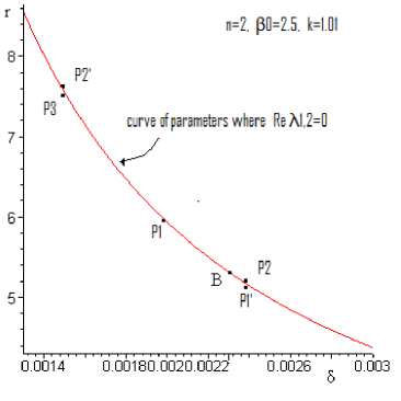
Figure 2: Curve of points $(\delta,r)$ where $Re\lambda_{1,2}=0$, for $n=2,\,\beta_{0}=2.5,\,k=1.01$, the point of Bautin bifurcation (point $B$), and the points chosen for numerical integration.

In order to put into light the behavior of the solution, that is qualitatively described in the bifurcation diagram, for a chosen point in the parameters space, we have to take several initial functions situated at different distances from the equilibrium point. We took the initial function $\phi$ of the form $\phi=x_{2}+c\,e^{\mu s}\cos(\omega s),$ where $\lambda_{\alpha 1,2}=\mu\pm i\omega$ are the eigenvalues of the linearized problem at the chosen parameters, and $c$ is a new parameter, that we vary.

The results of the integrations, for each of the considered points and for some choices of $c$ are represented vs time, but also in $x(t),\,\dot{x}(t)$ plots.

We consider first the solutions for two points $P_{1},\,P_{1}^{\prime}$ in the zone of the $(\delta,\,r)$ plane, corresponding to the zone 1 of the bifurcation diagram. More precisely the point $P_{1}$ has the coordinates $\delta=0.002,\;r=5.93,$ while for $P_{1}^{\prime},\,\delta=0.0024,\,r=5.14$ (see Fig. 2).

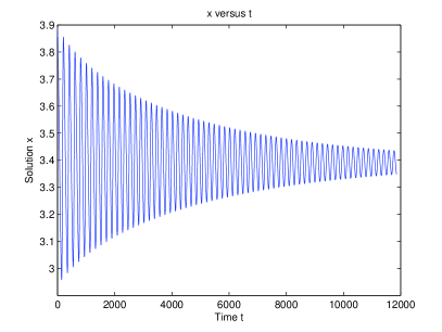
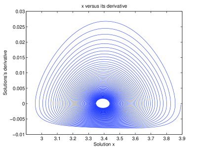
Figure 3: Phase portrait for the parameters in the point $P_{1}$, for $c=0.5$.

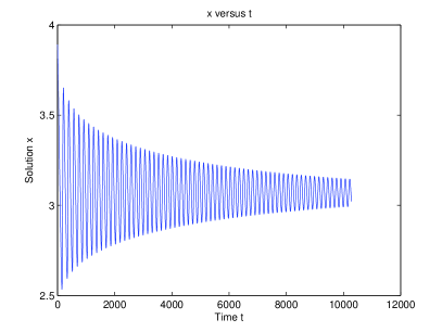
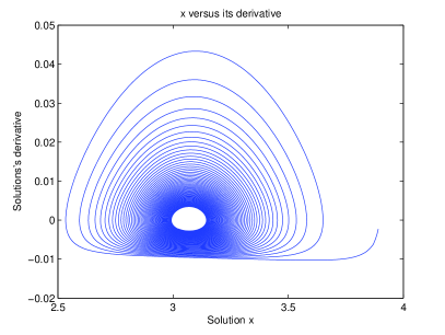
Figure 4: Phase portrait for the parameters in the point $P_{1}^{\prime}$, for $c=0.5$.

The behavior of the solution for these two points is that corresponding to an attracting focus. Since we obtained qualitatively the same image for several values of $c$, we represent only one of these, that for $c=0.5$, in Figs. 3 and 4.

The two points considered next, $P_{2}\,(\delta=0.0024,\,r=5.2)$ and $P_{2}^{\prime}\,(\delta=0.0015,\,r=7.56)$ are situated in the zone corresponding to zone 2 of the bifurcation diagram (see Fig. 2).

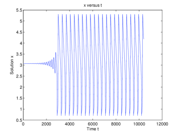
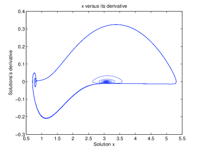
Figure 5: Phase portrait for the parameters in the point $P_{2}$, for $c=0.001$.

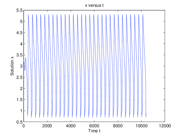
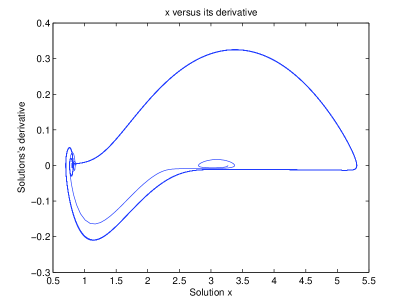
Figure 6: Phase portrait for the parameters in the point $P_{2}$, for $c=0.2$.

We see in Figs. 5 - 6 that a stable limit cycle occurs by Hopf bifurcation. In these two figures we present the behavior of the solution corresponding to $P_{2}$ and $c=0.001,$ respectively $c=0.2$. In Figs. 7 and 8 we present the behavior of the solution corresponding to $P_{2}^{\prime}$ and $c=0.1,$ respectively $c=5$.

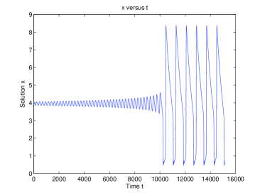
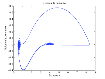
Figure 7: Phase portrait for the parameters in the point $P_{2}^{\prime}$, for $c=0.1$.

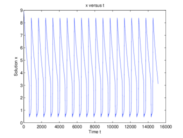
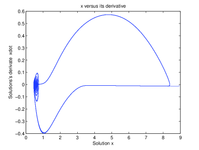
Figure 8: Phase portrait for the parameters in the point $P_{2}^{\prime}$, for $c=5$.

We remark that at each oscillation, on this limit cycle, at the end of a descending branch, in the $x$ versus $t$ representations, a small superposed oscillation occurs, that produces a little spiral in the left of the $x$ versus $\dot{x}$ representation. The moment when the solutions enters on this limit cycle depends on the distance between the initial function and $x_{2}$.

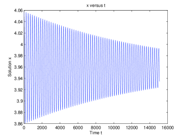
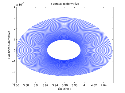
Figure 9: Phase portrait for the parameters in the point $P_{3}$, for $c=0.1$.

It was very difficult to find a point in the parameter plane, presenting the behavior corresponding to that of zone 3 of the bifurcation diagram. We suppose this is so because of the curve $T$ that is deformed and may be very close to the curve $\omega=0$. However, we found that for the point $P_{3}\,(d=0.0015,\,r=7.55),$ the behavior of the solution is the following: for initial functions close to $x_{2}$, that is $c\leq 0.42,$ the solution spirals towards $x_{2}$, while for $c\geq 0.425$ it is visible that the solution spirals away from a repulsive limit cycle, having increasing (with time) amplitude. When time increases, the solution tends to a large attractive limit cycle (that was previously formed by Hopf bifurcation when passing from zone 1 to zone 2). This types of behavior are shown in Figs. 9-13 where we took $c=0.1,\,c=0.42,\,c=0.425,\,c=0.45,\,c=0.6.$ In Figs. 10 and 11 the repulsive limit cycle is clearly visible, while in Figs. 12 and 13 the exterior attractive cycle is present.

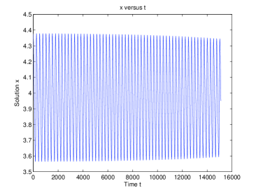
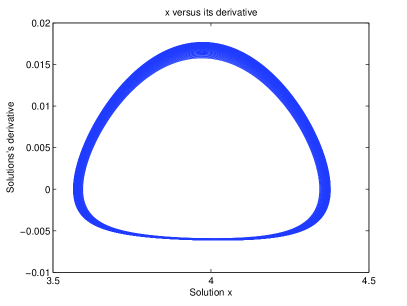
Figure 10: Phase portrait for the parameters in the point $P_{3}$, for $c=0.42$.

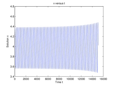
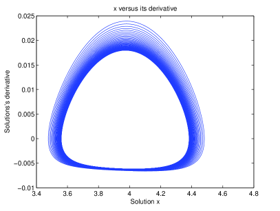
Figure 11: Phase portrait for the parameters in the point $P_{3}$, for $c=0.425$.

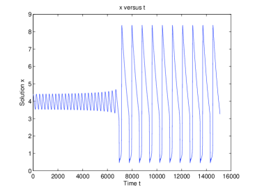
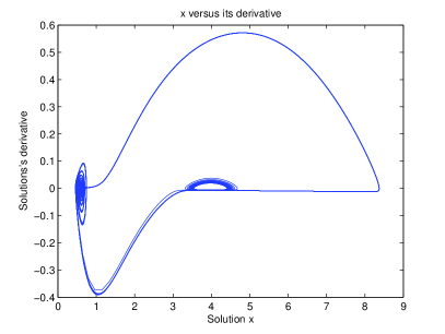
Figure 12: Phase portrait for the parameters in the point $P_{3}$, for $c=0.45$.

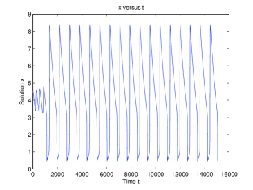
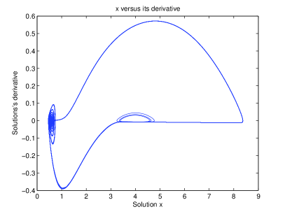
Figure 13: Phase portrait for the parameters in the point $P_{3}$, for $c=0.6$.

Hence, by numerical integrations we confirmed that the Bautin bifurcation, predicted by theoretical considerations, actually takes place, for the considered differential delay equation, in one of the points with $\l_{1}=0,\,l_{2}<0.$

It is important to remark that a consequence of the Bautin bifurcation is, for a certain zone in the parameter space, the occurrence of a repulsive limit cycle inside an attractive one. There, the behavior of the solution of eq. (1) strongly depends on the initial function. If the initial function is close to the equilibrium point $x_{2}$, the solution spirals towards $x_{2},$ while if the initial function is “far” from $x_{2}$, it will spiral towards the exterior stable limit cycle. From the point of view of the studied illness these two behaviors are quite different and this shows the importance of being able to control the initial condition.

References

- [1] T. Faria, Normal forms for RFDE in finite dimensional spaces -section 8.3 of J. Hale, L.T. Magalhaez, W. Oliva, Dynamics in infinite dimensions, Applied Mathematical Sciences, 47, Springer, New York, 2002.
- [2] J. Hale, S. M. Verduyn Lunel, Introduction to functional differential equation, Applied Mathematical Sciences, 99, Springer, New York, 2003.
- [3] A. V. Ion, On the Bautin bifurcation for systems of delay differential equations, Acta Univ. Apulensis, 8(2004), 235-246 (Proc. of ICTAMI 2004, Thessaloniki, Greece); arXiv:1111.1559.
- [4] A. V. Ion, New results concerning the stability of equilibria of a delay differential equation modeling leukemia, Proceedings of The 12th Symposium of Mathematics and its Applications, Timişoara, November 5-7, 2009, 375-380; arXiv:1001.4658.
- [5] A. V. Ion, R. M. Georgescu, Stability of equilibrium and periodic solutions of a delay equation modeling leukemia, Works of the Middle Volga Mathematical Society, 11(2009); arXiv:1001.5354.
- [6] A. V. Ion, R. M. Georgescu, Hopf points of codimension two in a delay differential equation modeling leukemia, arXiv:1205.3917.
- [7] Y. A. Kuznetsov, Elements of applied bifurcation theory, Applied Mathematical Sciences, 112, Springer, New York, 1998.
- [8] N. V. Minh, J. Wu, Invariant manifolds of partial functional equations, J. Diff. Eqns, 198, 2(2004), 381-421,
- [9] L. Pujo-Menjouet, M. C. Mackey, Contribution to the study of periodic chronic myelogenous leukemia, C. R. Biologies, 327(2004), 235-244.
- [10] L. Pujo-Menjouet, S. Bernard, M. C. Mackey, Long period oscillations in a model of hematopoietic stem cells, SIAM J. Applied Dynamical Systems, 2, 4(2005), 312-332.
- [11] J. Sotomayor, L. F. Mello, Lyapunov coefficients for degenerate Hopf bifurcation, arXiv:0709.3949.