Extracting Energy from an External Magnetic Field

Abstract

In this paper we describe the theory of a device that is able to extract energy from an external magnetic field. The device is a cylindrical magnetic insulator that once put in rotation makes electromagnetic angular momentum to be stored in the electromagnetic field in contrary direction to the mechanical angular momentum of the device. As a consequence due to total angular momentum conservation the device increases its angular velocity (when $\mathbf{\varepsilon\mu}>1$) and all conservation laws are rigorously satisfied.  The voltage generated by the device is found solving explicitly Maxwell equations for rotating magnetic insulators in external fields a subject that have provoked lots of polemics in the literature and which we hope to be here clarified due to our pedagogical presentation.

1 Introduction

In this paper we introduce the theory of a device that can in principle extract energy from an external magnetic field. The idea for the device came to us from the theoretical analysis of the 1913 Wilson & Wilson [21] experiment (WWE) described in Section 5. Since the correct theoretical explanation of the experiment gave rise to controversies in the literature due to difficulties in properly applying Maxwell theory in rotating frames we decided to give a very pedagogical presentation for the problem of expressing Maxwell equations in a coordinate invariant way using the theory of differential forms. Then, using that formalism and the correct jumping conditions for the electromagnetic field variables between moving boundaries separating two different media we get in a very clear way the electromagnetic field as measured in the laboratory in the WWE. We think that our approach clears up immediately what is wrong with some other attempts to find a correct description of the WWE in the sample of papers quoted. The description of the machine to extract energy from an external magnetic field is given in section 6 where it is observed that the machine once puts in motion makes electromagnetic angular to be stocked in the electric plus magnetic fields in the opposite direction of the mechanical angular mechanical of the device (when $\mathbf{\mu\varepsilon}>1$) and thus due to angular momentum conservation the machine has its mechanical angular momentum increased. Of course, all the conservation laws are in operation in our device and the energy being generated comes from the external electromagnetic field.

2 Maxwell Equations

The formulation of Maxwell equations in intrinsic form requires as preliminary mathematical structures:

(i) a $4$-dimensional orientable manifold $M$, the bundle of non homogeneous differential forms ${\textstyle\bigwedge}T^{\ast}M={\textstyle\bigoplus\nolimits_{r=0}^{r=4}}{\textstyle\bigwedge^{r}}T^{\ast}M$, where ${\textstyle\bigwedge^{r}}T^{\ast}M$ is the bundle of $r$-forms and

(ii) the differential operator $d:{\textstyle\bigwedge^{r}}T^{\ast}M\rightarrow{\textstyle\bigwedge^{r+1}}T^{\ast}M$, $d^{2}=0$.

Indeed, Maxwell equations deals with a field $F\in\sec{\textstyle\bigwedge^{2}}T^{\ast}M$ which is exact, i.e., $F=dA$, where $A\in\sec{\textstyle\bigwedge^{1}}T^{\ast}M$ and a current $\mathbf{J}\in\sec{\textstyle\bigwedge^{3}}T^{\ast}M$ that is also exact, i.e., $\mathbf{J}=dH$, where $H\in\sec{\textstyle\bigwedge^{2}}T^{\ast}M$. The set of equations

$$dF=0,\text{ \ \ }dH=-\mathbf{J},$$ (1)

is known as Maxwell equations and of course, we have

$$d\mathbf{J}=0,$$ (2)

i.e., the current is conserved.

Maxwell equations are invariant under diffeomorphisms as it happens with all theories formulated with differential forms. This means that if $h:M\rightarrow M$ is a diffeomorphism, then denoting as usual the pullback mapping by $h^{\ast}$, since the differential $d$ commutes with the pullback, i.e., $dh^{\ast}=h^{\ast}d$ we have that the fields $F^{\prime}=h^{\ast}F,H^{\prime}=h^{\ast}H,\mathbf{J}^{\prime}=h^{\ast}\mathbf{J}$ satisfy

$$dF^{\prime}=0,\text{ \ \ }dH^{\prime}=-\mathbf{J}^{\prime}.$$ (3)

Note that we did not make until now any requirements concerning the topology of manifold $M$, so to proceed we take arbitrary coordinates $\langle x^{\mu}\rangle$ covering $U\subset M$ and denoting $\langle e_{\mu}=\boldsymbol{\partial}/\boldsymbol{\partial}x^{\mu}=\boldsymbol{\partial}_{\mu}\rangle$ the corresponding coordinate basis for $TU$ and by $\langle\vartheta^{\mu}=dx^{\mu}\rangle$ the basis for $T^{\ast}U$ dual to the basis $\langle e_{\mu}\rangle$ we write

$$F =\frac{1}{2}F_{\mu\nu}\vartheta^{\mu}\wedge\vartheta^{\nu},$$

$$H =\frac{1}{2}H_{\mu\nu}\vartheta^{\mu}\wedge\vartheta^{\nu},$$ (4)

$$\mathbf{J} =\frac{1}{3!}J_{\mu\nu\rho}\vartheta^{\mu}\wedge\vartheta^{\nu}\boldsymbol{\wedge}\vartheta^{\nu}.$$

Maxwell equations are supposed to describe the behavior of electromagnetic fields in vacuum or in material media. But whereas, according to Feynman, the field $F$ is fundamental (it define the Lorentz force acting on probe charged particles moving in the field) the field $H$ is phenomenological. In fact, if we write Fourier representation for $F$ and $H,$

$$F_{\mu\nu}(x) ={\textstyle\int}d^{4}k\breve{F}_{\mu\nu}(k)e^{-i(k_{0}x^{0}+k_{1}x^{1}+k_{2}x^{2}+k_{3}x^{3})}:={\textstyle\int}d^{4}k\mathfrak{F}_{\mu\nu}(k,x),$$

$$H_{\mu\nu}(x) ={\textstyle\int}d^{4}k\text{ }\breve{H}_{\mu\nu}(k)e^{-i(k_{0}x^{0}+k_{1}x^{1}+k_{2}x^{2}+k_{3}x^{3})}:={\textstyle\int}d^{4}k\mathfrak{H}_{\mu\nu}(k,x),$$ (5)

in general we have, defining the 2-form valued function $\boldsymbol{\breve{\varkappa}}:\mathbb{R\times}\sec{\textstyle\bigwedge^{2}}T^{\ast}M\rightarrow\sec{\textstyle\bigwedge^{2}}T^{\ast}M$ (the frequency constituent equations of the medium) that

$$\mathfrak{H}(k_{0},x)=\boldsymbol{\breve{\varkappa}}(\mathfrak{F}(k_{0},x)).$$ (6)

The function $\boldsymbol{\breve{\varkappa}}$ may even be in some media a nonlinear function of $\mathfrak{F}$ (see, e.g., [2]) but in what follows we will consider only non dispersive media ($\boldsymbol{\breve{\varkappa}}$ is independent of $k_{0}$) in which case we can define a linear constituent function (an extensor field)

$$\boldsymbol{\varkappa}:\sec{\textstyle\bigwedge\nolimits^{2}}T^{\ast}M\rightarrow\sec{\textstyle\bigwedge\nolimits^{2}}T^{\ast}M,$$

$$H=\boldsymbol{\varkappa}(F).$$ (7)

In this case we have for the components $H_{\mu\nu}$ of $H$,

$$H_{\mu\nu}=\frac{1}{2}\boldsymbol{\varkappa}_{\mu\nu\cdot\cdot}^{\cdot\cdot\alpha\beta}F_{\alpha\beta}.$$ (8)

Of course, we have the obvious symmetries for the components of the constituent extensor $\boldsymbol{\varkappa}$,

$$\boldsymbol{\varkappa}_{\mu\nu\cdot\cdot}^{\cdot\cdot\alpha\beta}=-\boldsymbol{\varkappa}_{\nu\mu\cdot\cdot}^{\cdot\cdot\alpha\beta},\text{ \ \ }\boldsymbol{\varkappa}_{\mu\nu\cdot\cdot}^{\cdot\cdot\alpha\beta}=-\boldsymbol{\varkappa}_{\mu\nu\cdot\cdot}^{\cdot\cdot\beta\alpha},\text{ \ \ }\boldsymbol{\varkappa}_{\mu\nu\cdot\cdot}^{\cdot\cdot\alpha\beta}=\boldsymbol{\varkappa}_{\nu\mu\cdot\cdot}^{\cdot\cdot\beta\alpha}\text{ }.$$ (9)

2.1 Enter $\langle M,\boldsymbol{g},\mathbf{\nabla},\boldsymbol{\tau}_{\boldsymbol{g}},\uparrow\rangle$

We can proceed with the formulation of Maxwell theory without the introduction of additional mathematical objects in the manifold $M$. If you are interested in knowing the details, please consult [6]. From now on we will suppose that electromagnetic fields are to be described in a Lorentzian spacetime structure $\langle M,\boldsymbol{g},\mathbf{\nabla},\boldsymbol{\tau}_{\boldsymbol{g}},\uparrow\rangle$, where $\langle M,\boldsymbol{g}\boldsymbol{\rangle}$ is a Lorentzian manifold, $\mathbf{\nabla}$ is the Levi-Civita connection of $\boldsymbol{g}$, $\boldsymbol{\tau}_{\boldsymbol{g}}=\sqrt{\left|\det\boldsymbol{g}\right|}\boldsymbol{\vartheta}^{0}\wedge\boldsymbol{\vartheta}^{1}\wedge\boldsymbol{\vartheta}^{2}\wedge\boldsymbol{\vartheta}^{3}$ is the metrical volume element and $\uparrow$ denotes that the structure $\langle M,\boldsymbol{g)}$ is time orientable.

Remark 1

As it is well known a spacetime structure $(M,\boldsymbol{g},\mathbf{\nabla},\boldsymbol{\tau}_{\boldsymbol{g}},\uparrow\rangle$ when the Riemann curvature tensor of $\mathbf{\nabla}$ is non null represents a gravitational field generated by an energy-momentum tensor $T$ in Einstein’s General Relativity (GR) where Einstein equation is satisfied. It is a simple exercise to find an effective spacetime structure, say $\langle M,\mathbf{g},\mathbf{\nabla},\boldsymbol{\tau}_{\mathbf{g}},\uparrow\rangle$, to describe some material media. However, such structure has nothing to do with GR.

2.1.1 Reference Frames

We shall need in what follows the concepts of reference frames, observers and naturally adapted coordinate systems to a reference frame in a general Lorentzian spacetime structure $\langle M,\boldsymbol{g},\mathbf{\nabla},\boldsymbol{\tau}_{\boldsymbol{g}},\uparrow\rangle$.

We define a reference frame in $U\subset M$ as a unit timelike vector field $\boldsymbol{Z}$ pointing to the future. We have

$$\boldsymbol{g}(\boldsymbol{Z},\boldsymbol{Z})=1.$$ (10)

An observer is defined as a timelike curve $\sigma$ in $M$ (parametrized with proper time) and pointing to the future. We denote by $\sigma_{\ast s}$ the tangent vector at $\sigma(s)$ and

$$\boldsymbol{g}(\sigma_{\ast s},\sigma_{\ast s})=1.$$ (11)

We immediately realize that each one of the integral lines of $\boldsymbol{Z}$, is an observer.

Finally we say that coordinates $\langle x^{\mu}\rangle$ covering $U\subset M$ is a naturally adapted coordinate system to a reference frame $\boldsymbol{Z}$ (nacs$|$$\boldsymbol{Z}$) if

$$\boldsymbol{Z}=\frac{1}{\sqrt{g_{00}}}\frac{\boldsymbol{\partial}}{\boldsymbol{\partial}x^{0}}\text{ }.$$ (12)

A detailed classification of reference frames in a Lorentzian spacetime may be found, e.g., in [15]. For a classification of reference frames in a Riemann-Cartan spacetime, see, e.g., [3].

2.1.2 Formulation of Vacuum Maxwell Equations in $\langle M,\boldsymbol{g},\mathbf{\nabla},\boldsymbol{\tau}_{\boldsymbol{g}},\uparrow\rangle$

Given the structure $\langle M,\boldsymbol{g},\mathbf{\nabla},\boldsymbol{\tau}_{\boldsymbol{g}},\uparrow\rangle$ it is convenient to define

$$G=\underset{\boldsymbol{g}}{\star}^{-1}H$$ (13)

where $\underset{\boldsymbol{g}}{\star}:\sec{\textstyle\bigwedge\nolimits^{r}}T^{\ast}M\rightarrow\sec{\textstyle\bigwedge\nolimits^{4-r}}T^{\ast}M$ is the Hodge star operator and $\underset{\boldsymbol{g}}{\star}^{-1}\underset{\boldsymbol{g}}{\star}=\underset{\boldsymbol{g}}{\star}\underset{\boldsymbol{g}}{\star}^{-1}=\mathrm{Id}$. It is also a standard practice to introduce $J\in\sec{\textstyle\bigwedge\nolimits^{1}}T^{\ast}M$ such that

$$\mathbf{J=}\underset{\boldsymbol{g}}{\star}J.$$ (14)

We define also the (ex)tensor field

$$\boldsymbol{\chi}:\sec{\textstyle\bigwedge\nolimits^{2}}T^{\ast}M\rightarrow\sec{\textstyle\bigwedge\nolimits^{2}}T^{\ast}M,$$ (15)

$$G=\boldsymbol{\chi}(F).$$

Writing

$$G=\frac{1}{2}G_{\mu\nu}\vartheta^{\mu}\wedge\vartheta^{\nu}=\frac{1}{2}G^{\mu\nu}\vartheta_{\mu}\wedge\vartheta_{\nu}$$ (16)

we have

$$G_{\mu\nu}=\frac{1}{2}\chi_{\mu\nu\cdot\cdot}^{\cdot\cdot\alpha\beta}F_{\alpha\beta},\text{ \ \ }G^{\mu\nu}=\frac{1}{2}\chi^{\mu\nu\alpha\beta}F_{\alpha\beta}$$ (17)

and of course, the components of the constituent extensor $\boldsymbol{\chi}$ satisfy

$$\chi^{\mu\nu\alpha\beta}=-\chi^{\nu\mu\alpha\beta},\text{ \ \ }\chi^{\mu\nu\alpha\beta}=-\chi^{\mu\nu\beta\alpha},\text{ \ \ }\chi^{\mu\nu\alpha\beta}=\chi^{\nu\mu\beta\alpha}.$$ (18)

In vacuum the relation between the fields $G$ and $F$ is

$$G=F$$ (19)

and we write Maxwell equations as

$$dF=0,\text{ \ \ \ \ }d\underset{\boldsymbol{g}}{\star}F=-\underset{\boldsymbol{g}}{\star}J.$$ (20)

or better yet, applying the inverse of the Hodge star operator to both members of the non homogenous equation we can write

$$dF=0,\text{ \ \ \ \ }\underset{\boldsymbol{g}}{\delta}F=-J$$

We recall that

$$\underset{\boldsymbol{g}}{\star}\vartheta^{\mu_{1}...\mu_{p}}=\frac{1}{(n-p)!}\sqrt{\left|\det\boldsymbol{g}\right|}g^{\mu_{1}\nu_{1}}...g^{\mu_{p}\nu_{p}}\epsilon_{\nu_{1}...\nu_{n}}\vartheta^{\nu_{p+1}...\nu_{n}}.$$ (21)

Then, write

$$H=\underset{\boldsymbol{g}}{\star}F=\frac{1}{2}H_{\rho\sigma}\vartheta^{\rho}\wedge\vartheta^{\sigma}=\frac{1}{2}H^{\rho\sigma}\vartheta_{\rho}\wedge\vartheta_{\sigma}$$ (22)

and let us calculate $\underset{\boldsymbol{g}}{\star}F$. We have

$$\underset{\boldsymbol{g}}{\star}F =\frac{1}{2}F_{\mu\nu}\underset{\boldsymbol{g}}{\star}(\vartheta^{\mu}\wedge\vartheta^{\nu})$$

$$=\frac{1}{2}\frac{1}{2}F_{\mu\nu}\sqrt{\left|\det\boldsymbol{g}\right|}g^{\mu\alpha}g^{\nu\beta}\epsilon_{\alpha\beta\rho\sigma}\vartheta^{\rho}\wedge\vartheta^{\sigma}.$$ (23)

From Eq.(22) and Eq.(23) we have

$$H_{\rho\sigma} =\frac{1}{2}\sqrt{\left|\det\boldsymbol{g}\right|}g^{\mu\alpha}g^{\nu\beta}\epsilon_{\alpha\beta\rho\sigma}F_{\mu\nu}$$ (24)

$$=\frac{1}{2}\sqrt{\left|\det\boldsymbol{g}\right|}g^{\mu\alpha}g^{\nu\beta}\epsilon_{\rho\sigma\alpha\beta}F_{\mu\nu}$$

$$=\frac{1}{2}\sqrt{\left|\det\boldsymbol{g}\right|}\epsilon_{\rho\sigma\cdot\cdot}^{\cdot\cdot\mu\nu}F_{\mu\nu},$$

or taking into account that

$$H_{\rho\sigma}=\text{ }^{\ast}G_{\rho\sigma}=\frac{1}{2}\sqrt{\left|\det\boldsymbol{g}\right|}\epsilon_{\rho\sigma\cdot\cdot}^{\cdot\cdot\mu\nu}G_{\mu\nu}$$ (25)

we get

$$G^{\rho\sigma}=g^{\rho\mu}g^{\sigma\nu}F_{\mu\nu}=\frac{1}{2}(g^{\rho\mu}g^{\sigma\nu}-g^{\rho\nu}g^{\sigma\mu})F_{\mu\nu}.$$ (26)

Comparing this equation with Eq.(17) gives for the components $\varkappa^{\rho\sigma\mu\nu}$ of the constitutive (ex)tensor of the vacuum

$$\chi^{\rho\sigma\mu\nu}=(g^{\rho\mu}g^{\sigma\nu}-g^{\rho\nu}g^{\sigma\mu}).$$ (27)

Remark 2

Before proceeding let us recall that the similarity between the components of $\chi^{\rho\sigma\mu\nu}$ and the components $\boldsymbol{R}^{\rho\sigma\mu\nu}$ of a Riemann curvature tensor $\boldsymbol{R}$ with a $\boldsymbol{constant}$ Riemann curvature scalar $K$. Indeed, we have

$$\boldsymbol{R}^{\rho\sigma\mu\nu}=\frac{K}{12}(g^{\rho\mu}g^{\sigma\nu}-g^{\rho\nu}g^{\sigma\mu})$$ (28)

and thus $K=R=\delta_{\beta}^{\nu}R_{\cdot\cdot\alpha\nu}^{\alpha\beta\cdot\cdot}$. Take notice that $\boldsymbol{R}$ is not the Riemann curvature tensor of the Levi-Civita connection $D$ of $\boldsymbol{g}$.

Exercise 3

Show that in components Maxwell equations $dF=0$, $dH=-\underset{\boldsymbol{g}}{\star}J$  when $\boldsymbol{\varkappa}$ has its vacuum value read

$$\partial_{\mu}F_{\alpha\beta}+\partial_{\beta}F_{\mu\alpha}+\partial_{\alpha}F_{\beta\mu} =0,$$ (29)

$$\frac{1}{\sqrt{\left|\det\boldsymbol{g}\right|}}\partial_{\mu}(\sqrt{\left|\det\boldsymbol{g}\right|}F^{\mu\nu}) =J^{\nu}.$$ (30)

Solution 4

We have

$$dF =\frac{1}{2}d(F_{\alpha\beta}\wedge\vartheta^{\alpha}\wedge\vartheta^{\beta})$$

$$=\frac{1}{2}\partial_{\mu}F_{\alpha\beta}\vartheta^{\mu}\wedge\vartheta^{\alpha}\wedge\vartheta^{\beta}$$

$$=\frac{1}{3!}(\partial_{\mu}F_{\alpha\beta}+\partial_{\beta}F_{\mu\alpha}+\partial_{\alpha}F_{\beta\mu})\vartheta^{\mu}\wedge\vartheta^{\alpha}\wedge\vartheta^{\beta}$$

and Eq.(29) follows.

Next we define $J=J_{\mu}\vartheta^{\mu}:=\rho\vartheta^{0}-j_{i}\vartheta^{i}$ and get

$$\underset{\boldsymbol{g}}{\star}J=\frac{1}{3!}\sqrt{\left|\det\boldsymbol{g}\right|}J_{\lambda}g^{\lambda\kappa}\epsilon_{\kappa\mu\alpha\beta}\vartheta^{\mu}\wedge\vartheta^{\alpha}\wedge\vartheta^{\beta}.$$ (31)

Then the equation $dH=-\underset{\boldsymbol{g}}{\star}J$ reads

$$\frac{1}{3!}(\partial_{\mu}H_{\alpha\beta}+\partial_{\beta}H_{\mu\alpha}+\partial_{\alpha}H_{\beta\mu})\vartheta^{\mu}\wedge\vartheta^{\alpha}\wedge\vartheta^{\beta}=-\frac{1}{3!}\sqrt{\left|\det\boldsymbol{g}\right|}J^{\kappa}\epsilon_{\kappa\mu\alpha\beta}\vartheta^{\mu}\wedge\vartheta^{\alpha}\wedge\vartheta^{\beta}$$ (32)

and

$$(\partial_{\mu}H_{\alpha\beta}+\partial_{\beta}H_{\mu\alpha}+\partial_{\alpha}H_{\beta\mu})=-\sqrt{\left|\det\boldsymbol{g}\right|}J^{\kappa}\epsilon_{\kappa\mu\alpha\beta}.$$ (33)

Multiplying both members of the last equation by $\epsilon^{{}_{\lambda\mu\alpha\beta}}$ and recalling that

$$\epsilon^{{}_{\lambda\mu\alpha\beta}}\epsilon_{\kappa\mu\alpha\beta} =3!\delta_{\kappa}^{\lambda}$$ (34)

$$\epsilon^{{}_{\lambda\mu\alpha\beta}}\epsilon_{\alpha\beta\kappa\iota} =2!\delta_{\kappa\iota}^{\lambda\mu}$$

we have

$$\epsilon^{{}_{\lambda\mu\alpha\beta}}(\partial_{\mu}H_{\alpha\beta}+\partial_{\beta}H_{\mu\alpha}+\partial_{\alpha}H_{\beta\mu})=-3!\sqrt{\left|\det\boldsymbol{g}\right|}J^{\lambda}.$$ (35)

Now,

$$\epsilon^{{}_{\lambda\mu\alpha\beta}}\partial_{\mu}H_{\alpha\beta} =\partial_{\mu}(\frac{1}{2}\sqrt{\left|\det\boldsymbol{g}\right|}\epsilon^{{}_{\lambda\mu\alpha\beta}}\epsilon_{\alpha\beta\kappa\iota}F^{\kappa\iota})$$

$$=\partial_{\mu}(\sqrt{\left|\det\boldsymbol{g}\right|}\delta_{\kappa\iota}^{\lambda\mu}F^{\kappa\iota})$$

$$=2\partial_{\mu}(\sqrt{\left|\det\boldsymbol{g}\right|}F^{\lambda\mu})$$

$$=-2\partial_{\mu}(\sqrt{\left|\det\boldsymbol{g}\right|}F^{\mu\lambda}).$$ (36)

Analogous calculations give that the other two terms in the first member of Eq.(35) are also equal to $-2\partial_{\mu}(\sqrt{\left|\det\boldsymbol{g}\right|}F^{\mu\lambda})$. Then Eq.(35) becomes

$$\frac{1}{\sqrt{\left|\det\boldsymbol{g}\right|}}\partial_{\mu}(\sqrt{\left|\det\boldsymbol{g}\right|}F^{\mu\lambda})=J^{\lambda}$$

and Eq.(30) is proved.

Remark 5

We present yet another simple proof of Eq.(30) which however presumes the knowledge of the Clifford calculus. We introduce the Dirac operator $\boldsymbol{\partial=}\vartheta^{\mu}\mathbf{\nabla}_{\boldsymbol{\partial/\partial}x^{\mu}}$ and recall that $dM=\boldsymbol{\partial}\wedge M$ for any $M\in\sec{\textstyle\bigwedge}T^{\ast}M\hookrightarrow\sec\mathcal{C}\ell(M,\mathtt{g})$ where $\mathcal{C}\ell(M,\mathtt{g})$ is the Clifford bundle of differential forms. We have

$$dH=d\underset{\boldsymbol{g}}{\star}G=\boldsymbol{\partial}\wedge\underset{\boldsymbol{g}}{\star}G=-\underset{\boldsymbol{g}}{\star}J$$

Now, we calculate $\boldsymbol{\partial}\wedge\underset{\boldsymbol{g}}{\star}G=\boldsymbol{\partial}\wedge(\tilde{G}\boldsymbol{\tau}_{\boldsymbol{g}})$ in orthonormal basis $\{\boldsymbol{e}_{\mathbf{a}}\}$ for $TU$ and dual basis $\{\boldsymbol{\theta}^{\mathbf{a}}\}$ for $T^{\ast}U$ with $U\subset M$. We have

$$d\underset{\boldsymbol{g}}{\star}G =\boldsymbol{\partial}\wedge(\tilde{G}\boldsymbol{\tau}_{\boldsymbol{g}})$$

$$=-\boldsymbol{\theta}^{\mathbf{a}}\wedge(\mathbf{\nabla}_{\boldsymbol{e}_{\mathbf{a}}}(G\boldsymbol{\tau}_{\boldsymbol{g}}))$$

$$=-\frac{1}{2}\left(\boldsymbol{\theta}^{\mathbf{a}}\mathbf{\nabla}_{\boldsymbol{e}_{\mathbf{a}}}(G\boldsymbol{\tau}_{\boldsymbol{g}})+\mathbf{\nabla}_{\boldsymbol{e}_{\mathbf{a}}}(G\boldsymbol{\tau}_{\boldsymbol{g}})\boldsymbol{\theta}^{\mathbf{a}}\right)$$

$$=-\frac{1}{2}\left(\boldsymbol{\theta}^{\mathbf{a}}(\mathbf{\nabla}_{\boldsymbol{e}_{\mathbf{a}}}G)\boldsymbol{\tau}_{\boldsymbol{g}}+\boldsymbol{\theta}^{\mathbf{a}}G(\mathbf{\nabla}_{\boldsymbol{e}_{\mathbf{a}}}\boldsymbol{\tau}_{\boldsymbol{g}})+(\mathbf{\nabla}_{\boldsymbol{e}_{\mathbf{a}}}G)\boldsymbol{\tau}_{\boldsymbol{g}}\boldsymbol{\theta}^{\mathbf{a}}+G(\mathbf{\nabla}_{\boldsymbol{e}_{\mathbf{a}}}\boldsymbol{\tau}_{\boldsymbol{g}})\boldsymbol{\theta}^{a}\right)$$

$$=-\frac{1}{2}\left(\boldsymbol{\theta}^{\mathbf{a}}(\mathbf{\nabla}_{\boldsymbol{e}_{\mathbf{a}}}G)-(\mathbf{\nabla}_{\boldsymbol{e}_{\mathbf{a}}}G)\boldsymbol{\theta}^{\mathbf{a}})\boldsymbol{\tau}_{\boldsymbol{g}}-\frac{1}{2}\boldsymbol{(}-\boldsymbol{\theta}^{\mathbf{a}}G(\mathbf{\nabla}_{\boldsymbol{e}_{\mathbf{a}}}\boldsymbol{\tau}_{\boldsymbol{g}})-G(\mathbf{\nabla}_{\boldsymbol{e}_{\mathbf{a}}}\boldsymbol{\tau}_{\boldsymbol{g}})\boldsymbol{\theta}^{\mathbf{a}}\right).$$

But

$$-\frac{1}{2}\left(\boldsymbol{\theta}^{\mathbf{a}}(\mathbf{\nabla}_{\boldsymbol{e}_{\mathbf{a}}}G)-(\mathbf{\nabla}_{\boldsymbol{e}_{\mathbf{a}}}G)\boldsymbol{\theta}^{\mathbf{a}})\boldsymbol{\tau}_{\boldsymbol{g}}\right)=-(\boldsymbol{\partial\lrcorner}G)\boldsymbol{\tau}_{\boldsymbol{g}}$$

and

$$\mathbf{\nabla}_{\boldsymbol{e}_{\mathbf{a}}}\boldsymbol{\tau}_{\boldsymbol{g}}=\mathbf{\nabla}_{\boldsymbol{e}_{\mathbf{a}}}(\boldsymbol{\theta}^{\mathbf{0}}\wedge\boldsymbol{\theta}^{\mathbf{1}}\wedge\boldsymbol{\theta}^{\mathbf{2}}\wedge\boldsymbol{\theta}^{\mathbf{3}})=-\Gamma_{\cdot\mathbf{a0}}^{\mathbf{0\cdot\cdot}}\boldsymbol{\tau}_{\boldsymbol{g}}-\Gamma_{\cdot\mathbf{a1}}^{\mathbf{1\cdot\cdot}}\boldsymbol{\tau}_{\boldsymbol{g}}-\Gamma_{\cdot\mathbf{a2}}^{\mathbf{2\cdot\cdot}}\boldsymbol{\tau}_{\boldsymbol{g}}-\Gamma_{\cdot\mathbf{a3}}^{\mathbf{3\cdot\cdot}}\boldsymbol{\tau}_{\boldsymbol{g}}=0,$$

because

$$\Gamma_{\cdot\mathbf{a0}}^{\mathbf{0\cdot\cdot}}=\Gamma_{\cdot\mathbf{a1}}^{\mathbf{1\cdot\cdot}}=\Gamma_{\cdot\mathbf{a1}}^{\mathbf{1\cdot\cdot}}=\Gamma_{\cdot\mathbf{a1}}^{\mathbf{1\cdot\cdot}}=0.$$

Then,

$$-(\boldsymbol{\partial\lrcorner}G)\boldsymbol{\tau}_{\boldsymbol{g}}=-J\boldsymbol{\tau}_{\boldsymbol{g}}$$

or

$$\boldsymbol{\partial\lrcorner}G=J.$$ (37)

Now,

$$\boldsymbol{\partial\lrcorner}G =\frac{1}{2}\vartheta^{\mu}\lrcorner(D_{\mu}G^{\alpha\beta}\vartheta_{\alpha}\wedge\vartheta_{\beta})=D_{\mu}G^{\mu\beta}\vartheta_{\beta}$$

$$=(\partial_{\mu}G^{\mu\beta}+\Gamma_{\cdot\mu\kappa}^{\mu\cdot\cdot}G^{\kappa\beta}+\Gamma_{\cdot\mu\kappa}^{\beta\cdot\cdot}G^{\mu\kappa})\vartheta_{\beta}$$

$$=(\partial_{\mu}G^{\mu\beta}+\Gamma_{\cdot\mu\kappa}^{\mu\cdot\cdot}G^{\kappa\beta})\vartheta_{\beta}=(\partial_{\mu}G^{\mu\beta}+\frac{\partial_{\mu}\sqrt{\left|\det\boldsymbol{g}\right|}}{\sqrt{\left|\det\boldsymbol{g}\right|}}G^{\mu\beta})\vartheta_{\beta}$$

$$=\frac{1}{\sqrt{\left|\det\boldsymbol{g}\right|}}\partial_{\mu}(\sqrt{\left|\det\boldsymbol{g}\right|}G^{\mu\beta})\vartheta_{\beta},$$

and we get recalling that in vacuum $G=F$

$$\frac{1}{\sqrt{\left|\det\boldsymbol{g}\right|}}\partial_{\mu}(\sqrt{\left|\det\boldsymbol{g}\right|}F^{\mu\beta})=J^{\beta}$$

which is Eq.(30) again.

3 Maxwell Equations in Minkowski Spacetime

3.1 Vacuum Case

We next suppose that electromagnetic phenomena take place in a non dispersive material medium in Minkowski spacetime, i.e., the structure $M=\langle\mathbb{R}^{4},\boldsymbol{\mathring{g}},\mathbf{\mathring{\nabla}},\boldsymbol{\tau}_{\boldsymbol{\mathring{g}}},\uparrow\rangle$. Since the Riemann curvature of  the Levi-Civita connection $\mathbf{\mathring{\nabla}}$ is null (i.e., $\boldsymbol{\mathring{R}}(\mathbf{\mathring{\nabla}})=0$) there exists global coordinates $\langle\mathtt{x}^{\mu}\rangle$ such that denoting by $\langle\boldsymbol{e}_{\mu}=\boldsymbol{\partial}/\boldsymbol{\partial}\mathtt{x}^{\mu}\rangle$ a basis for $TM$ and $\langle\gamma^{\mu}=d\mathtt{x}^{\mu}\rangle$ the basis of $T^{\ast}M$ dual to $\langle\boldsymbol{e}_{\mu}\rangle$ we have

$$\boldsymbol{\mathring{g}}=\mathtt{\eta}_{\mu\nu}\gamma^{\mu}\otimes\gamma^{\nu}$$ (38)

where the matrix with entries $\eta_{\mu\nu}$ being the diagonal matrix diag$(1,-1,-1,-1)$.

In this case the components of constitutive (extensor) $\boldsymbol{\chi}$ of the vacuum in the (nacs$|$$I$) $\{\mathtt{x}^{\mu}\}$ to the inertial frame $\boldsymbol{L}=\boldsymbol{e}_{0}=\boldsymbol{\partial}/\boldsymbol{\partial}\mathtt{x}^{0}$ are

$$\mathfrak{\chi}^{\rho\sigma\mu\nu}=(\mathtt{\eta}^{\rho\mu}\mathtt{\eta}^{\sigma\nu}-\mathtt{\eta}^{\rho\nu}\mathtt{\eta}^{\sigma\mu}).$$ (39)

Thus

$$\mathtt{G}^{\rho\sigma}=\frac{1}{2}(\mathtt{\eta}^{\rho\mu}\mathtt{\eta}^{\sigma\nu}-\mathtt{\eta}^{\rho\nu}\mathtt{\eta}^{\sigma\mu})\mathring{F}_{\mu\nu}=\mathtt{\eta}^{\rho\mu}\mathtt{\eta}^{\sigma\nu}\mathtt{F}_{\mu\nu}.$$ (40)

Denoting by $(\mathtt{F}_{\mu\nu})$ and $(\mathtt{G}^{\rho\sigma})$, respectively, the matrices with elements $\mathtt{F}_{\mu\nu}$ and $\mathtt{G}^{\rho\sigma}$ we have

$$(\mathtt{F}_{\mu\nu})=\left(\begin{array}[c]{cccc}0&\mathtt{E}_{1}&\mathtt{E}_{2}&\mathtt{E}_{3}\\ -\mathtt{E}_{1}&0&-\mathtt{B}_{3}&\mathtt{B}_{2}\\ -\mathtt{E}_{2}&\mathtt{B}_{3}&0&-\mathtt{B}_{1}\\ -\mathtt{E}_{3}&-\mathtt{B}_{2}&\mathtt{B}_{1}&0\end{array}\right),\qquad(\mathtt{G}^{\rho\sigma})=\left(\begin{array}[c]{cccc}0&-\mathtt{B}_{1}&-\mathtt{B}_{2}&-\mathtt{B}_{3}\\ \mathtt{B}_{1}&0&\mathtt{E}_{3}&-\mathtt{E}_{2}\\ \mathtt{B}_{2}&-\mathtt{E}_{3}&0&\mathtt{E}_{1}\\ \mathtt{B}_{3}&\mathtt{E}_{2}&-\mathtt{E}_{1}&0\end{array}\right).$$

Of course, Maxwell equations in coordinates in the Einstein-Lorentz Poincaré gauge reads

$$\frac{\partial\mathtt{F}_{\alpha\beta}}{\partial\mathtt{x}^{\mu}}+\frac{\partial\mathtt{F}_{\mu\alpha}}{\partial\mathtt{x}^{\beta}}+\frac{\partial\mathtt{F}_{\beta\mu}}{\partial\mathtt{x}^{\alpha}}=0,$$ (41)

and

$$\frac{\partial\mathtt{F}^{\mu\nu}}{\partial\mathtt{x}^{\mu}}=\mathtt{J}^{\nu}.$$ (42)

3.2 Non Dispersive Homogeneous and Isotropic Linear Medium Case

We suppose in what follows that a linear non dispersive homogeneous and isotropic medium (NDHILM) is at rest in a given reference frame $\boldsymbol{V}$ in $U\subset M$ which has an arbitrary motion relative to the laboratory frame that is here modelled by the inertial frame $\boldsymbol{L}=\boldsymbol{e}_{0}=\boldsymbol{\partial}/\boldsymbol{\partial}\mathtt{x}^{0}$. Let $\langle x^{\prime\mu}\rangle$ be coordinate functions covering $U$ that are (nacs$|$$\boldsymbol{V}$) and $\langle\boldsymbol{\partial/}\boldsymbol{\partial}x^{\prime\mu}\rangle$ be a basis for $TU$ and $\langle\vartheta^{\prime\mu}=dx^{\prime\mu}\rangle$ the corresponding dual basis for $T^{\ast}M$. Writing in this case

$$\boldsymbol{\mathring{g}}=\mathring{g}_{\mu\nu}^{\prime}\vartheta^{\prime\mu}\otimes\vartheta^{\prime\nu}=\mathtt{\eta}_{\mu\nu}\gamma^{\mu}\wedge\gamma\boldsymbol{\vartheta}^{\nu},$$ (43)

we have

$$\boldsymbol{V}=V^{\prime\mu}\boldsymbol{\partial}/\boldsymbol{\partial}x^{\prime\mu}=\frac{1}{\sqrt{\mathring{g}_{00}^{\prime}}}\boldsymbol{\partial}/\boldsymbol{\partial}x^{\prime 0}=\mathtt{V}^{\mu}\boldsymbol{\partial}/\boldsymbol{\partial}\mathtt{x}^{\mu}=\mathtt{V}^{0}\frac{\boldsymbol{\partial}}{\boldsymbol{\partial}\mathtt{x}^{0}}+\mathtt{V}^{i}\frac{\boldsymbol{\partial}}{\boldsymbol{\partial}\mathtt{x}^{i}}.$$ (44)

We now write

$$F =\frac{1}{2}F_{\rho\sigma}^{\prime}\vartheta^{\prime\rho}\wedge\vartheta^{\prime\sigma}=\frac{1}{2}F^{\prime\rho\sigma}\vartheta_{\rho}^{\prime}\wedge\vartheta_{\sigma}^{\prime}$$

$$=\frac{1}{2}\mathtt{F}_{\rho\sigma}\gamma^{\rho}\wedge\gamma^{\sigma}=\frac{1}{2}\mathtt{F}^{\rho\sigma}\gamma_{\rho}\wedge\gamma_{\sigma},$$

$$G =\frac{1}{2}G_{\rho\sigma}^{\prime}\vartheta^{\prime\rho}\wedge\vartheta^{\prime\sigma}=\frac{1}{2}G^{\prime\rho\sigma}\vartheta_{\rho}^{\prime}\wedge\vartheta_{\sigma}^{\prime}$$

$$=\frac{1}{2}\mathtt{G}_{\rho\sigma}\gamma^{\rho}\wedge\gamma^{\sigma}=\frac{1}{2}\mathtt{G}^{\rho\sigma}\gamma_{\rho}\wedge\gamma_{\sigma}.$$ (45)

We use the following notations for the elements of the matrices $(\mathtt{F}_{\rho\sigma}),(F_{\rho\sigma})$ $(\mathtt{G}_{\rho\sigma})$ and $(G_{\rho\sigma}^{\prime})$ as

$$(\mathtt{F}_{\rho\sigma}) =\left(\begin{array}[c]{cccc}0&\mathtt{E}_{1}&\mathtt{E}_{2}&\mathtt{E}_{3}\\ -\mathtt{E}_{1}&0&-\mathtt{B}_{3}&\mathtt{B}_{2}\\ -\mathtt{E}_{2}&\mathtt{B}_{3}&0&-\mathtt{B}_{1}\\ -\mathtt{E}_{3}&-\mathtt{B}_{2}&\mathtt{B}_{1}&0\end{array}\right),\text{ \ \ }(F_{\rho\sigma}^{\prime})=\left(\begin{array}[c]{cccc}0&E_{1}^{\prime}&E_{2}^{\prime}&E_{3}^{\prime}\\ -E_{1}^{\prime}&0&-B_{3}^{\prime}&B_{2}^{\prime}\\ -E_{2}^{\prime}&B_{3}^{\prime}&0&-B_{1}^{\prime}\\ -E_{3}^{\prime}&-B_{2}^{\prime}&B_{1}^{\prime}&0\end{array}\right),$$ (54)

$$(\mathtt{G}_{\rho\sigma}) =\left(\begin{array}[c]{cccc}0&\mathtt{D}_{1}&\mathtt{D}_{2}&\mathtt{D}_{3}\\ -\mathtt{D}_{1}&0&-\mathtt{H}_{3}&\mathtt{H}_{2}\\ -\mathtt{D}_{2}&\mathtt{H}_{3}&0&-\mathtt{H}_{1}\\ -\mathtt{D}_{3}&-\mathtt{H}_{2}&\mathtt{H}_{1}&0\end{array}\right),\text{ \ \ }(G_{\rho\sigma}^{\prime})=\left(\begin{array}[c]{cccc}0&D_{1}^{\prime}&D_{2}^{\prime}&D_{3}^{\prime}\\ -D_{1}^{\prime}&0&-H_{3}^{\prime}&H_{2}^{\prime}\\ -D_{2}^{\prime}&H_{3}^{\prime}&0&-H_{1}^{\prime}\\ -D_{3}^{\prime}&-H_{2}^{\prime}&H_{1}^{\prime}&0\end{array}\right).$$ (63)

Then Maxwell equations read in the coordinates $\langle x^{\prime\mu}\rangle$ (which are a (nacs$|$$\boldsymbol{V}$)):

$$\frac{\partial F_{\alpha\beta}^{\prime}}{\partial x^{\prime\mu}}+\frac{\partial F_{\mu\alpha}^{\prime}}{\partial x^{\prime\beta}}+\frac{\partial F_{\beta\mu}^{\prime}}{\partial x^{\prime\alpha}}=0,$$

and

$$\frac{1}{\sqrt{\left|\det\boldsymbol{\mathring{g}}\right|}}\frac{\partial}{\partial x^{\prime\alpha}}\left(\frac{1}{\sqrt{\left|\det\boldsymbol{\mathring{g}}\right|}}\mathring{g}^{{}^{\prime}\alpha\rho}\mathring{g}^{\prime\beta\sigma}G_{\rho\sigma}^{\prime}\right)=J^{\prime\beta}.$$

3.3 Minkowski Relations

We want now to define using differential forms the concepts of electric and magnetic fields and induction fields in a NDHILM.

Given an arbitrary reference frame $\boldsymbol{Z}$ in Minkowski spacetime let $\boldsymbol{z=\mathring{g}(Z},)$ be the physically equivalent $1$-form field.

Definition 6

The electric $\underset{\boldsymbol{z}}{\boldsymbol{E}}$ and the magnetic $\underset{\boldsymbol{z}}{\boldsymbol{B}}$ $1$-form fields and the $\underset{\boldsymbol{z}}{\boldsymbol{D}}$ and $\underset{\boldsymbol{z}}{\boldsymbol{H}}$ $1$-form fields according to the observers at rest in $\boldsymbol{Z}$ are:

$$\underset{\boldsymbol{z}}{\boldsymbol{E}} :=\boldsymbol{z}\lrcorner F,\text{ \ \ \ \ \ \ \ }\underset{\boldsymbol{z}}{\boldsymbol{B}}:=\boldsymbol{z}\lrcorner\star F,$$ (64)

$$\underset{\boldsymbol{z}}{\boldsymbol{D}} :=\boldsymbol{z}\lrcorner G,\text{ \ \ \ \ \ \ \ }\underset{\boldsymbol{z}}{\boldsymbol{H}}:=\boldsymbol{z}\lrcorner\star G.$$ (65)

We immediately have

$$F =\boldsymbol{z\wedge}\underset{\boldsymbol{z}}{\boldsymbol{E}}-\star(\boldsymbol{z}\wedge\underset{\boldsymbol{z}}{\boldsymbol{B}}),$$ (66)

$$G =\boldsymbol{z\wedge}\underset{\boldsymbol{z}}{\boldsymbol{D}}-\star(\boldsymbol{z}\wedge\underset{\boldsymbol{z}}{\boldsymbol{H}}).$$ (67)

Let $\boldsymbol{V}$ be an arbitrary reference frame in Minkowski spacetime ($\boldsymbol{v=\mathring{g}(V},)$) where the NDHILM is at rest.

Definition 7

The electric $\underset{\boldsymbol{v}}{\boldsymbol{D}}$ and the magnetic $\underset{\boldsymbol{v}}{\boldsymbol{H}}$ $1$-form fields according to the observers at rest in $\boldsymbol{Z}$ are related with the $\underset{\boldsymbol{v}}{\boldsymbol{E}}\,\,{\mbox{and}}\,\,\underset{\boldsymbol{v}}{\boldsymbol{B}}$ by:

$$\underset{\boldsymbol{v}}{\boldsymbol{D}}:=\boldsymbol{\varepsilon}\underset{\boldsymbol{v}}{\boldsymbol{E}}\qquad\text{and}\qquad\underset{\boldsymbol{v}}{\boldsymbol{H}}:=\frac{1}{\boldsymbol{\mu}}\underset{\boldsymbol{v}}{\boldsymbol{B}}.$$ (68)

We immediately have

$$G=\frac{1}{\boldsymbol{\mu}}\left(\boldsymbol{\varepsilon\mu}-1\right)[\boldsymbol{v\wedge}(\boldsymbol{v}\lrcorner F)]+\frac{1}{\boldsymbol{\mu}}F.$$ (69)

which will be called Minkowski constitutive relation.

Exercise 8

Prove Eq.(69).

Solution 9

From Eq.(67) and Definition 7 we have

$$G=\varepsilon\boldsymbol{v}\wedge(\boldsymbol{v}\lrcorner F)-\frac{1}{\mu}\star[\boldsymbol{v}\wedge(\boldsymbol{v}\lrcorner\star F)]$$ (70)

Now using the identities Eq.(156) and Eqs.(157) in the Appendix we have

$$\star[\boldsymbol{v}\wedge(\boldsymbol{v}\lrcorner\star F)] =\star[\boldsymbol{v}\wedge\star(\boldsymbol{v}\wedge F)]=\star\star[\boldsymbol{v}\lrcorner(\boldsymbol{v}\wedge F)]=-\boldsymbol{v}\lrcorner(\boldsymbol{v}\wedge F)$$

$$=-(\boldsymbol{v}\lrcorner\boldsymbol{v)}F+\boldsymbol{v}\wedge(\boldsymbol{v}\lrcorner F)$$

and then

$$G =\varepsilon\boldsymbol{v}\wedge(\boldsymbol{v}\lrcorner F)+\frac{1}{\mu}[F-\boldsymbol{v}\wedge(\boldsymbol{v}\lrcorner F)]$$

$$=\frac{1}{\mu}\left(\varepsilon\mu-1\right)[\boldsymbol{v\wedge}(\boldsymbol{v}\lrcorner F)]+\frac{1}{\mu}F.$$

3.3.1 Coordinate Expression for Minkowski Constitutive Relations

We want now to express Minkowski constitutive relations in arbitrary $\{x^{\mu}\}$ coordinates covering $U\subset M$ and let $F_{\lambda\mu}$, $G_{\mu\nu}$ and $v^{\mu}$ be the components of $F$, $G$ and the reference frame $\boldsymbol{V}$ in an arbitrary natural bases $\{\boldsymbol{\partial}_{\mu}=\boldsymbol{\partial/\partial}x^{\mu}\}$ and $\{\vartheta^{\mu}=dx^{\mu}\}$. Let us calculate $\boldsymbol{v}\lrcorner G$. We have

$$\boldsymbol{v}\lrcorner G=\left(\varepsilon-\frac{1}{\mu}\right)\boldsymbol{v}\lrcorner[\boldsymbol{v\wedge}(\boldsymbol{v}\lrcorner F)]+\frac{1}{\mu}\boldsymbol{v}\lrcorner F.$$

From identity Eq.(156) in Appendix we have

$$\boldsymbol{v}\lrcorner[\boldsymbol{v\wedge}(\boldsymbol{v}\lrcorner F)] =(\boldsymbol{v}\lrcorner\boldsymbol{v})(\boldsymbol{v}\lrcorner F)]-\boldsymbol{v\wedge(v}\wedge(\boldsymbol{v}\lrcorner F))$$

$$=\boldsymbol{v}\lrcorner F-(\boldsymbol{v\wedge v})\wedge(\boldsymbol{v}\lrcorner F))$$

$$=\boldsymbol{v}\lrcorner F.$$ (71)

Then

$$\boldsymbol{v}\lrcorner G=\boldsymbol{\varepsilon v}\lrcorner F$$ (72)

and in components Eq.(72) is

$$v^{\mu}\vartheta_{\mu}\lrcorner\left(\frac{1}{2}G_{\alpha\beta}\vartheta^{\alpha}\wedge\vartheta^{\beta}\right)=\boldsymbol{\varepsilon}v^{\mu}\vartheta_{\mu}\lrcorner\left(\frac{1}{2}F_{\alpha\beta}\vartheta^{\alpha}\wedge\vartheta^{\beta}\right)$$

and since $\vartheta_{\mu}\lrcorner\left(\frac{1}{2}G_{\alpha\beta}\vartheta^{\alpha}\wedge\vartheta^{\beta}\right)=G_{\mu\nu}\vartheta^{\nu}$, $\vartheta_{\mu}\lrcorner\left(\frac{1}{2}F_{\alpha\beta}\vartheta^{\alpha}\wedge\vartheta^{\beta}\right)=F_{\mu\nu}\vartheta^{\nu}$ we have

$$v^{\mu}G_{\mu\nu}=\boldsymbol{\varepsilon}v^{\mu}F_{\mu\nu}.$$ (73)

Let us now calculate $\boldsymbol{v}\lrcorner\star G$. First we note that

$$\star G=\left(\boldsymbol{\varepsilon}-\frac{1}{\boldsymbol{\mu}}\right)\star[\boldsymbol{v\wedge}(\boldsymbol{v}\lrcorner F)]+\frac{1}{\boldsymbol{\mu}}\star F$$

and using the same steps as the ones leading to Eq.(72) we first get

$$\boldsymbol{v}\lrcorner\star[\boldsymbol{v\wedge}(\boldsymbol{v}\lrcorner F)]=\star[\boldsymbol{v\wedge}(\boldsymbol{v}\wedge(\boldsymbol{v\lrcorner}F))]=\star(\boldsymbol{v\wedge v)\wedge}(\boldsymbol{v\lrcorner}F)=0$$

and then

$$\boldsymbol{v}\lrcorner\star G=\frac{1}{\boldsymbol{\mu}}\boldsymbol{v}\lrcorner\star F.$$ (74)

Now,

$$\star F =\frac{1}{2}\left(\frac{1}{2}\sqrt{\left|\det\boldsymbol{\mathring{g}}\right|}F^{\mu\nu}\varepsilon_{\mu\nu\rho\sigma}\vartheta^{\rho}\wedge\vartheta^{\sigma}\right),$$

$$\star G =\frac{1}{2}\left(\frac{1}{2}\sqrt{\left|\det\boldsymbol{\mathring{g}}\right|}G^{\mu\nu}\varepsilon_{\mu\nu\rho\sigma}\vartheta^{\rho}\wedge\vartheta^{\sigma}\right)$$

and

$$\boldsymbol{v}\lrcorner\star F =\frac{1}{2}\sqrt{\left|\det\boldsymbol{\mathring{g}}\right|}v^{\kappa}F^{\mu\nu}\varepsilon_{\mu\nu\kappa\sigma}\vartheta^{\sigma},$$

$$\boldsymbol{v}\lrcorner\star G =\frac{1}{2}\sqrt{\left|\det\boldsymbol{\mathring{g}}\right|}v^{\kappa}G^{\mu\nu}\varepsilon_{\mu\nu\kappa\sigma}\vartheta^{\sigma}$$

and finally Eq.(74) reads in components

$$\boldsymbol{\mu}v^{\kappa}G^{\mu\nu}\varepsilon_{\mu\nu\kappa\sigma}=v^{\kappa}F^{\mu\nu}\varepsilon_{\mu\nu\kappa\sigma}$$ (75)

or in equivalent forms

$$\boldsymbol{\mu}v_{\kappa}G_{\mu\nu}\varepsilon^{\mu\nu\kappa\sigma} =v_{\kappa}F_{\mu\nu}\varepsilon^{\mu\nu\kappa\sigma},$$

$$\boldsymbol{\mu}\varepsilon^{\mu\nu\kappa\sigma}G_{\mu\nu}\mathring{g}_{\kappa\iota}v^{\iota} =\varepsilon^{\mu\nu\kappa\sigma}F_{\mu\nu}\mathring{g}_{\kappa\iota}v^{\iota}.$$ (76)

3.3.2 Polarization, Magnetization, Bound Current and Bound Charge Fields

We define moreover the polarization $2-$form field $\Pi$ by

$$\Pi:F-G.$$ (77)

Given an arbitrary frame $\boldsymbol{Z}$ we decompose $\Pi$ as

$$\Pi:=\boldsymbol{z\wedge}\underset{\boldsymbol{z}}{\boldsymbol{P}}-\star(\boldsymbol{z}\wedge\underset{\boldsymbol{z}}{\boldsymbol{M}}),$$ (78)

where $\underset{\boldsymbol{z}}{\boldsymbol{P}}$ and $\underset{\boldsymbol{z}}{\boldsymbol{M}}$ are called respectively the polarization $1$-form field and magnetization $1$-form field in $\boldsymbol{Z}$. Moreover, from Eq.(68) and Eq.(69) we get

$$\underset{\boldsymbol{z}}{\boldsymbol{P}}=\underset{\boldsymbol{z}}{\boldsymbol{E}}-\underset{\boldsymbol{z}}{\boldsymbol{D}}\text{ \ and\ \ }\underset{\boldsymbol{z}}{\boldsymbol{M}}=\underset{\boldsymbol{z}}{\boldsymbol{B}}-\underset{\boldsymbol{z}}{\boldsymbol{H}}.$$

From the non homogeneous Maxwell equation $d\star G=-\mathbf{J}$ we have

$$d\star F=-\mathbf{J}+d\star\Pi.$$ (79)

The field

$$\mathcal{J}:=-d\star\Pi$$ (80)

is called the bound current $3$-form. Given an arbitrary frame $\boldsymbol{Z}$ we decompose $\mathcal{J}$ as

$$\mathcal{J}:=\boldsymbol{z\wedge}\underset{\boldsymbol{z}}{\mathcal{J}}+\underset{\boldsymbol{z}}{\mathcal{\rho}}$$ (81)

where $\underset{\boldsymbol{z}}{\mathcal{J}}$ is called the bound current $2$-form field and $\underset{\boldsymbol{z}}{\mathcal{\rho}}$ is called the bound charge $3$-form field.

In the coordinates $\langle\mathtt{x}^{\mu}\rangle$ and $\langle x^{\prime\mu}\rangle$ respectively adapted to the inertial laboratory frame $\boldsymbol{L=e}_{\mathbf{0}}$ and to an arbitrary frame $\boldsymbol{V}$ we write

$$\Pi =\frac{1}{2}\mathtt{\Pi}_{\rho\sigma}\mathbf{\vartheta}^{\rho}\wedge\mathbf{\vartheta}^{\sigma}=\frac{1}{2}\mathtt{\Pi}^{\rho\sigma}\mathbf{\vartheta}_{\rho}\wedge\mathbf{\vartheta}_{\sigma}$$

$$=\frac{1}{2}\Pi_{\rho\sigma}^{\prime}\vartheta^{\prime\rho}\wedge\vartheta^{\prime\sigma}=\frac{1}{2}\Pi^{\prime\rho\sigma}\vartheta_{\rho}^{\prime}\wedge\vartheta_{\sigma}^{\prime},$$ (82)

where the entries of the matrices $(\mathring{\Pi}_{\rho\sigma})$ and $(\Pi_{\rho\sigma})$ are, respectively,

$$(\mathtt{\Pi}_{\rho\sigma}):=\left(\begin{array}[c]{cccc}0&-\mathtt{P}_{1}&-\mathtt{P}_{2}&-\mathtt{P}_{3}\\ \mathtt{P}_{1}&0&-\mathtt{M}_{3}&\mathtt{M}_{2}\\ \mathtt{P}_{2}&\mathtt{M}_{3}&0&-\mathtt{M}_{1}\\ \mathtt{P}_{3}&-\mathtt{M}_{2}&\mathtt{M}_{1}&0\end{array}\right),\text{ \ \ }(\Pi_{\rho\sigma}):=\left(\begin{array}[c]{cccc}0&-P_{1}^{\prime}&-P_{2}^{\prime}&-P_{3}^{\prime}\\ P_{1}^{\prime}&0&-M_{3}^{\prime}&M_{2}^{\prime}\\ P_{2}^{\prime}&M_{3}^{\prime}&0&-M_{1}^{\prime}\\ P_{3}^{\prime}&-M_{2}^{\prime}&M_{1}^{\prime}&0\end{array}\right)$$ (83)

3.4 Constitutive Relations in a Uniformly Rotating Frame $\boldsymbol{V}$.

We introduce besides the coordinates $\{\mathtt{x}^{\mu}\}$ also cylindrical coordinates $\langle x^{\mu}\rangle$ in $\mathbb{R}^{4}-\{0\}$ which are also (nacs$|$$\boldsymbol{L}=\boldsymbol{e}_{0}$). As usual we write

$$\mathtt{x}^{0} =x^{0},$$

$$\mathtt{x}^{1} =x^{1}\cos x^{2},$$

$$\mathtt{x}^{2} =x^{1}\sin x^{2},$$

$$\mathtt{x}^{3} =x^{3}.$$ (84)

We will simplify the notation when convenient by writing $\{\mathtt{x}^{0},\mathtt{x}^{1},\mathtt{x}^{2},\mathtt{x}^{3}\}:=\{t,\mathtt{x},\mathtt{y},\mathtt{z}\}$ and $\{x^{0},x^{1},x^{2},x^{3}\}:=\{t,r,\phi,z\}$.

Next we introduce a particular rotating reference frame $\boldsymbol{V}\in\sec TM$ in Minkowski spacetime:

$$\boldsymbol{V=}\frac{1}{\sqrt{1-\mathtt{v}^{2}}}\frac{\boldsymbol{\partial}}{\boldsymbol{\partial}t}+\frac{\omega}{\sqrt{1-\mathtt{v}^{2}}}\left(-\mathtt{y}\frac{\boldsymbol{\partial}}{\boldsymbol{\partial}\mathtt{x}}+\mathtt{x}\frac{\boldsymbol{\partial}}{\boldsymbol{\partial}\mathtt{y}}\right)$$ (85)

where

$$\mathtt{v}:=\sqrt{\mathtt{v}_{\mathtt{x}}^{2}+\mathtt{v}_{\mathtt{y}}^{2}}=\omega r,$$ (86)

with $\omega$ the (classical) angular velocity of $\boldsymbol{V}$ relative to the inertial laboratory frame $\boldsymbol{L=e}_{0}$.

Since

$$\frac{\boldsymbol{\partial}}{\boldsymbol{\partial}\phi}=-y\frac{\boldsymbol{\partial}}{\boldsymbol{\partial}x}+x\frac{\boldsymbol{\partial}}{\boldsymbol{\partial}y}$$ (87)

we can also write taking into account that $\gamma=1/\sqrt{1-\mathtt{v}^{2}}$,

$$\boldsymbol{V} =\frac{1}{\sqrt{1-\mathtt{v}^{2}}}\frac{\boldsymbol{\partial}}{\boldsymbol{\partial}t}+\frac{\omega}{\sqrt{1-\mathtt{v}^{2}}}\frac{\boldsymbol{\partial}}{\boldsymbol{\partial}\phi}$$

$$=\gamma\left(\boldsymbol{\partial}_{t}+\mathtt{v}\frac{1}{r}\boldsymbol{\partial}_{\phi}\right)$$ (88)

and

$$\boldsymbol{v:=\mathring{g}}(\boldsymbol{V},\text{ })=\gamma\left(dt+\mathtt{v}rd\phi\right).$$ (89)

Remark 10

It is important to recall that although the coordinates $\{t,r,\phi,z\}$ cover $\mathbb{R}^{4}-\{0\}$ the reference frame $\boldsymbol{V}$ if realized by a physical system can only have material support for $r<1/\omega$.

We introduce next the vector field

$$\mathbf{v} =-\omega\mathtt{y}\boldsymbol{\partial}_{\mathtt{x}}+\omega\mathtt{x}\boldsymbol{\partial}_{\mathtt{y}}$$

$$=\mathtt{v}\frac{1}{r}\boldsymbol{\partial}_{\phi}=\mathtt{v}\boldsymbol{e}_{\phi}$$ (90)

It is quite obvious that the vector field $\mathbf{v}$ represents the classical $3$- velocity of a (material) point whose $3$-dimensional trajectory in the spacelike section $\mathbb{R}^{3}$ determined by $\boldsymbol{L=e}_{0}$ has parametric equations $(r\cos\omega t,r\sin\omega t,z_{0})$ where $z_{0}$ is an arbitrary real constant.

Take notice that in engineering notation the vector field $\mathbf{v}$ is usually denoted by $\vec{v}=\mathtt{v}\boldsymbol{\hat{e}}_{\phi}$. We will use engineering notation when convenient in some of the formulas that follows for pedagogical reasons.

A (nacs$|$$\boldsymbol{V}$)

Before we proceed we introduce explicitly the transformation law between the coordinates $\langle\mathtt{x}^{\mu}\rangle$ that are (nacs$|$$\boldsymbol{e}_{0}$) and $\langle x^{\prime\mu}\rangle$ that are (nacs$|$$\boldsymbol{V}$).

These are

$$\mathtt{x}^{0} =x^{\prime 0},$$

$$\mathtt{x}^{1} =x^{\prime 1}\cos\omega\mathtt{x}^{0}-x^{\prime 2}\sin\omega\mathtt{x}^{0},$$

$$\mathtt{x}^{2} =x^{\prime 1}\sin\omega\mathtt{x}^{0}+x^{\prime 2}\cos\omega\mathtt{x}^{0}.$$

$$\mathtt{x}^{3} =x^{\prime 3}.$$ (91)

To simplify the notation we will write $\{x^{\prime 0},x^{\prime 1},x^{\prime 2},x^{\prime 3}):=(t^{\prime},x^{\prime},y^{\prime},z^{\prime})$.

We define also cylindrical coordinates $\langle\hat{x}^{\prime\mu}\rangle$ naturally adapted to $\boldsymbol{V}$ by

$$x^{\prime 0} =\hat{x}^{\prime 0},$$ (92)

$$x^{\prime 1} =\hat{x}^{\prime 1}\cos\hat{x}^{\prime 2},$$

$$x^{\prime 2} =\hat{x}^{\prime^{\prime}1}\sin\hat{x}^{\prime 2},$$

$$x^{\prime 3} =\hat{x}^{\prime 3}.$$

We moreover simply the notation writing  $\{\hat{x}^{\prime 0},\hat{x}^{\prime 1},\hat{x}^{\prime 2},\hat{x}^{\prime 3}):=(t^{\prime},r^{\prime},\phi^{\prime},z^{\prime}).$

Now, it is trivial to see that

$$t^{\prime}=t,\text{ \ \ }r^{\prime}=r,\text{ \ \ }\phi^{\prime}=\phi-\omega t,\text{ \ \ }z^{\prime}=\mathtt{z}.$$ (93)

This has as consequence the  obvious relations

$$dt^{\prime}=dt,\text{ \ \ }dr^{\prime}=dr,\text{ \ \ }d\phi^{\prime}=d\phi-\omega dt,\text{ \ \ }dz^{\prime}=d\mathtt{z}$$ (94)

and the not so obvious ones

$$\frac{\boldsymbol{\partial}}{\boldsymbol{\partial}t^{\prime}}=\frac{\boldsymbol{\partial}}{\boldsymbol{\partial}t}+\omega\frac{\boldsymbol{\partial}}{\boldsymbol{\partial}\phi},\text{ \ \ }\frac{\boldsymbol{\partial}}{\boldsymbol{\partial}r^{\prime}}=\frac{\boldsymbol{\partial}}{\boldsymbol{\partial}r},\text{ \ \ }\frac{\boldsymbol{\partial}}{\boldsymbol{\partial}\phi^{\prime}}=\frac{\boldsymbol{\partial}}{\boldsymbol{\partial}\phi},\text{ \ \ }\frac{\boldsymbol{\partial}}{\boldsymbol{\partial}z^{\prime}}=\frac{\boldsymbol{\partial}}{\boldsymbol{\partial}\mathtt{z}}.$$ (95)

Then we see that

$$\boldsymbol{V}=\frac{1}{\sqrt{1-\mathtt{v}^{2}}}\frac{\boldsymbol{\partial}}{\boldsymbol{\partial}t^{\prime}}=\frac{1}{\sqrt{\mathring{g}_{00}}}\frac{\boldsymbol{\partial}}{\boldsymbol{\partial}t^{\prime}},$$ (96)

which shows that indeed $\langle\hat{x}^{\prime\mu}\rangle$ is a (nacs$|$$\boldsymbol{Z}$).

We also notice that since $r^{\prime}=r$ and $\frac{\boldsymbol{\partial}}{\boldsymbol{\partial}\phi^{\prime}}=\frac{\boldsymbol{\partial}}{\boldsymbol{\partial}\phi}$ we can write Eq.(90) as

$$\mathbf{v} =\omega\mathtt{v}\frac{1}{r}\frac{\boldsymbol{\partial}}{\boldsymbol{\partial}\phi}=\omega\mathtt{v}\frac{1}{r^{\prime}}\frac{\boldsymbol{\partial}}{\boldsymbol{\partial}\phi^{\prime}}=-\omega y^{\prime}\frac{\boldsymbol{\partial}}{\boldsymbol{\partial}x^{\prime}}+\omega x^{\prime}\frac{\boldsymbol{\partial}}{\boldsymbol{\partial}y^{\prime}}$$

$$=v_{x^{\prime}}\frac{\boldsymbol{\partial}}{\boldsymbol{\partial}x^{\prime}}+v_{y\prime}\frac{\boldsymbol{\partial}}{\boldsymbol{\partial}y^{\prime}}$$ (97)

$$=v_{1}^{\prime}\frac{\boldsymbol{\partial}}{\boldsymbol{\partial}x^{\prime 1}}+v_{2}^{\prime}\frac{\boldsymbol{\partial}}{\boldsymbol{\partial}x^{\prime 2}}.$$

We write the metric $\boldsymbol{\mathring{g}}$ using the coordinates $\langle x^{\mu}\rangle$ and $\langle\hat{x}^{\mu}\rangle$ as

$$\boldsymbol{\mathring{g}} =\mathring{g}_{\mu\nu}^{\prime}dx^{\prime\mu}\otimes dx^{\prime\nu}$$

$$=(1-\omega^{2}r^{\prime 2})dt^{\prime}\otimes dt^{\prime}+2\omega y^{\prime}dx^{\prime}\otimes dt^{\prime}-2\omega x^{\prime}dy\otimes dt^{\prime}-dx^{\prime}\otimes dx^{\prime}-dy^{\prime}\otimes dy^{\prime}$$

$$-dz^{\prime}\otimes dz^{\prime},$$ (98)

or

$$\boldsymbol{\mathring{g}} =\hat{g}_{\mu\nu}d\hat{x}^{\prime\mu}\otimes d\hat{x}^{\prime\nu}$$

$$=(1-\mathtt{v}^{2})dt\otimes dt-2\omega d\phi^{\prime}\otimes dt-dr^{\prime}\otimes dr^{\prime}-r^{\prime 2}d\phi^{\prime}\otimes d\phi^{\prime}-dz^{\prime}\otimes dz^{\prime}.$$ (99)

We immediately read from Eq.(98) that

$$\mathring{g}_{00}^{\prime}=(1-\mathtt{v}^{2})=1/\gamma^{2},\text{ \ \ }\mathring{g}_{10}^{\prime}=-v_{1}^{\prime}=\omega y^{\prime},\text{ \ \ }\mathring{g}_{20}^{\prime}=-v_{2}^{\prime}=\omega x^{\prime},\text{ \ \ }\mathring{g}_{30}^{\prime}=0.$$ (100)

After this (long) digression we return to Eq.(73) and Eq.(76) that in coordinates $\langle x^{\prime\mu}\rangle$ which is (nacs$|$$\boldsymbol{V}$), can be immediately written in the engineering format (of vector calculus) as:

$$\vec{D}^{\prime} =\boldsymbol{\varepsilon}\vec{E}^{\prime},$$ (101)

$$\boldsymbol{\mu}[\frac{1}{\gamma^{2}}\vec{H}^{\prime}-\vec{v}\times\vec{D}^{\prime}] =\boldsymbol{[}\frac{1}{\gamma^{2}}\vec{B}^{\prime}-\vec{v}\times\vec{E}^{\prime}].$$ (102)

Then, we finally get

$$\vec{D}^{\prime}=\boldsymbol{\varepsilon}\vec{E}^{\prime},$$ (103)

$$\vec{H}^{\prime}=\frac{1}{\boldsymbol{\mu}}[\vec{B}^{\prime}+\gamma^{2}(\boldsymbol{\varepsilon\mu}-1)\vec{v}\times\vec{E}^{\prime}].$$ (104)

The polarization and magnetization vector fields in engineering notation are, respectively, then:

$$\vec{P}^{\prime}=(\boldsymbol{\varepsilon}-1)\vec{E}^{\prime},$$ (105)

$$\vec{M}^{\prime}=(1-\frac{1}{\boldsymbol{\mu}})\vec{B}^{\prime}+\frac{1}{\boldsymbol{\mu}}\gamma^{2}(1-\boldsymbol{\varepsilon\mu})\vec{v}\times\vec{E}^{\prime}.$$ (106)

To obtain the expression of those fields in the laboratory (in coordinates $\langle\mathtt{x}^{\mu}\rangle$ naturally adapted to $\boldsymbol{l=e}_{0}=\boldsymbol{\partial}/\boldsymbol{\partial}\mathtt{x}^{0}=\boldsymbol{\partial}/\boldsymbol{\partial}t$) it is only necessary to recall that

$$F_{\mu\nu}^{\prime}=\frac{\partial\mathtt{x}^{\alpha}}{\partial x^{\prime\mu}}\frac{\partial\mathtt{x}^{\beta}}{\partial x^{\prime\nu}}\mathtt{F}_{\alpha\beta},\text{ \ \ }H_{\mu\nu}^{\prime}=\frac{\partial\mathtt{x}^{\alpha}}{\partial x^{\prime\mu}}\frac{\partial\mathtt{x}^{\beta}}{\partial x^{\prime\nu}}\mathtt{H}_{\alpha\beta},\text{ \ \ }\Pi_{\mu\nu}^{\prime}=\frac{\partial\mathtt{x}^{\alpha}}{\partial x^{\prime\mu}}\frac{\partial\mathtt{x}^{\beta}}{\partial x^{\prime\nu}}\Pi_{\alpha\beta}.$$ (107)

Now, from Eq.(91) we have

$$\left(\frac{\partial\mathtt{x}^{\alpha}}{\partial x^{\prime\mu}}\right)=\left(\begin{array}[c]{cccc}1&0&0&0\\ -\omega\mathtt{y}&\cos\omega t^{\prime}&-\sin\omega t^{\prime}&0\\ \omega\mathtt{x}&\sin\omega t^{\prime}&\cos\omega t^{\prime}&0\\ 0&0&0&1\end{array}\right).$$ (108)

Then, we have, e.g.,

$$E_{x}^{\prime} =\mathtt{E}_{\mathtt{x}}\cos\omega t+\mathtt{E}_{\mathtt{y}}\sin\omega t+\omega x^{\prime}\mathtt{B}_{\mathtt{z}},$$

$$E_{x}^{\prime} =-\mathtt{E}_{\mathtt{x}}\sin\omega t+\mathtt{E}_{\mathtt{y}}\cos\omega t+\omega y^{\prime}\mathtt{B}_{\mathtt{z}},$$

$$E_{z}^{\prime} =\mathtt{E}_{\mathtt{z}}-\omega\mathtt{yB}_{\mathtt{y}}-\omega\mathtt{xB}_{\mathtt{x}},$$

$$B_{x}^{\prime} =\mathtt{B}_{\mathtt{x}}\cos\omega t+\mathtt{B}_{\mathtt{y}}\sin\omega t,$$

$$B_{y}^{\prime} =-\mathtt{B}_{\mathtt{x}}\sin\omega t+\mathtt{B}_{\mathtt{y}}\cos\omega t,$$

$$B_{z}^{\prime} =\mathtt{B}_{\mathtt{z}}.$$ (109)

We recall also that writing at time $t$ in the laboratory the position vector of a point $p=(\mathtt{x},\mathtt{y},\mathtt{z})$ in engineering notation as $\mathtt{\vec{x}}=\mathtt{x}\boldsymbol{\hat{e}}_{\mathtt{x}}+\mathtt{y}\boldsymbol{\hat{e}}_{\mathtt{y}}+\mathtt{z}\boldsymbol{\hat{e}}_{\mathtt{z}}$ and the ($3$-dimensional) angular velocity field of the frame $\boldsymbol{V}$ as $\vec{\omega}=\Omega\boldsymbol{\hat{e}}_{\mathtt{z}}$ we have

$$\vec{v}=\vec{\Omega}\times\mathtt{\vec{x}.}$$ (110)

Finally we write the relation between the charge and current densities as observed in the laboratory and the rotating frame. From $J=J^{\prime\mu}\vartheta_{\mu}^{\prime}=J^{\mu}\gamma_{\mu}$, with $(J^{0},J^{1},J^{2},J^{3})=(\rho,j_{x},j_{y},j_{z})$ and $(J^{{}^{\prime}0},J^{{}^{\prime}1},J^{{}^{\prime}2},J^{\prime 3})=(\rho^{\prime},j_{x}^{\prime},j_{y}^{\prime},j_{z}^{\prime})$ we have

$$J^{\prime\mu}=\frac{\partial x^{\prime\mu}}{\partial x^{\alpha}}J^{\alpha},$$ (111)

which gives

$$\rho^{\prime} =\mathtt{\rho},$$ (112)

$$j_{x}^{\prime} =\omega y^{\prime}\mathtt{\rho}+\mathtt{j}_{\mathtt{x}}\cos\omega t+\mathtt{j}_{\mathtt{y}}\sin\omega t,$$ (113)

$$j_{y}^{\prime} =-\omega x^{\prime}\mathtt{\rho}-\mathtt{j}_{\mathtt{x}}\sin\omega t+\mathtt{j}_{\mathtt{y}}\cos\omega t,$$ (114)

$$j_{z}^{\prime} =\mathtt{j}_{\mathtt{z}}.$$ (115)

4 Jump Conditions for the Fields $F$ and $G$ at the Boundary of a Moving NDHILM

The interface between a moving NDHILM described by the velocity field $\boldsymbol{V}$ and the vacuum defines a hypersurface $\Sigma=0$ in Minkowski spacetime. The jump conditions can be deduced from Maxwell equations and are well known. A  very simple deduction of the discontinuity of the fields $\vec{E},\vec{B},\vec{D}$ and $\vec{H}$ is given in [10]. Here we write the jump conditions in differential form style for the case where the free current $\star J=0$. Denoting as usual by $[F]$, $[G]$ and $[\star G]$ the respective discontinuities of $F$, $G$ and $\star G$ at the boundary of medium and vacuum we have:

$$\left.[F]\wedge d\Xi\right|_{\Xi=0}=0,$$ (116)

$$\left.[G]\llcorner d\Xi\right|_{\Xi=0}=0.$$ (117)

Observe that $\left.[G]\llcorner d\Xi\right|_{\Xi=0}=0$ implies, of course

$$\star[\left.[G]\llcorner d\Xi\right|_{\Xi=0}]=-\star[\left.[G]\lrcorner d\Xi\right|_{\Xi=0}]=\left.[\star G]\wedge d\Xi\right|_{\Xi=0}=0.$$

Also, $\left.[F]\wedge d\Xi\right|_{\Xi=0}=$ $\left.d\Xi\wedge[F]\right|_{\Xi=0}=\left.\star(d\Xi\lrcorner\star F)\right|_{\Xi=0}=0$ and we can write the jump conditions also as:

$$\left.[\star F]\llcorner d\Xi\right|_{\Xi=0}=0,$$ (118)

$$\left.[\star G]\wedge d\Xi\right|_{\Xi=0}=0.$$ (119)

Now, in the (nacs$|$$\boldsymbol{L=e}_{0}$) $\langle\mathtt{x}^{\mu}\rangle$ we have

$$n:=d\Xi=\frac{\partial\Xi}{\partial\mathtt{x}^{\mu}}\boldsymbol{\vartheta}^{\mu}=n_{\mu}\boldsymbol{\vartheta}^{\mu}=n^{\mu}\boldsymbol{\vartheta}_{\mu}.$$ (120)

Define $\mathbf{n}:=-\frac{\partial\Xi}{\partial\mathtt{x}^{i}}\frac{\boldsymbol{\partial}}{\boldsymbol{\partial}\mathtt{x}^{i}}$ the spatial vector field  which is normal to the moving boundary $\Xi(\mathtt{t},\mathtt{x,y,z})=0$. Now, each spacial point of the moving boundary at time $\mathtt{t}$ has Newtonian velocity $\mathbf{v}$. Observe that during a time interval $\triangle\mathtt{x}^{0}=\triangle\mathtt{t}$ a point at the boundary with arbitrary coordinates $(\mathtt{x},\mathtt{y},\mathtt{z})$ will arrive at the point $(\mathtt{x}+v_{\mathtt{x}}\triangle\mathtt{t},\mathtt{y}+v_{\mathtt{y}}\triangle\mathtt{t},\mathtt{z}+v_{\mathtt{z}}\triangle\mathtt{t})$. The hypersurface $\Xi$  at $(\mathtt{t}+\mathtt{\triangle\mathtt{t}},\mathtt{x}+v_{\mathtt{x}}\triangle\mathtt{t},\mathtt{y}+v_{\mathtt{y}}\triangle\mathtt{t},\mathtt{z}+v_{\mathtt{z}}\triangle\mathtt{t})$ will satisfy

$$\Xi(\mathtt{t}+\mathtt{\triangle\mathtt{t}},\mathtt{x}+v_{\mathtt{x}}\triangle\mathtt{t},\mathtt{y}+v_{\mathtt{y}}\triangle\mathtt{t},\mathtt{z}+v_{\mathtt{z}}\triangle\mathtt{t})$$

$$=\Xi(\mathtt{t},\mathtt{x,y,z})+\left.\frac{\partial\Xi}{\partial\mathtt{x}^{\mu}}\right|_{(\mathtt{t,x,y,z)}}\triangle\mathtt{x}^{\mu}=0$$

$$=\triangle\mathtt{t}\left.\frac{\partial\Xi}{\partial\mathtt{t}}\right|_{(\mathtt{t,x,y,z)}}+v_{\mathtt{x}}\triangle\mathtt{t}\left.\frac{\partial\Xi}{\partial\mathtt{x}}\right|_{(\mathtt{t,x,y,z)}}+v_{\mathtt{y}}\triangle\mathtt{t}\left.\frac{\partial\Xi}{\partial\mathtt{y}}\right|_{(\mathtt{t,x,y,z)}}+\left.v_{\mathtt{z}}\triangle\mathtt{t}\frac{\partial\Xi}{\partial\mathtt{z}}\right|_{(\mathtt{t,x,y,z)}}=0.$$ (121)

Thus, we get in engineering notation taking into account that $\vec{n}=-\nabla\Xi$ that Eq.(121) implies

$$\frac{\partial\Xi}{\partial\mathtt{t}}-\vec{n}\bullet\vec{v}=0.$$ (122)

Then, we can write the jump conditions in its usual engineering notation as

$$\vec{n}\bullet[\underset{\boldsymbol{l}}{\vec{B}}] =0,\text{ \ \ \ }(\vec{n}\bullet\vec{v})[\underset{\boldsymbol{l}}{\vec{B}}]+\vec{n}\times[\underset{\boldsymbol{l}}{\vec{E}}]=0$$ (123)

$$\vec{n}\bullet[\underset{\boldsymbol{l}}{\vec{D}}] =0\text{, \ \ \ }(\vec{n}\bullet\vec{v})[\underset{\boldsymbol{l}}{\vec{D}}]+\vec{n}\times[\underset{\boldsymbol{l}}{\vec{H}}]=0.$$ (124)

Exercise 11

Show that Eq.(117) implies the formulas in Eq.(124).

Solution 12

We calculate $\left.[G]\llcorner d\Xi\right|_{\Xi=0}=\left.[G]\llcorner n\right|_{\Xi=0}=\left.n\lrcorner[G]\right|_{\Xi=0}=0$. Now, from Eq.(67) we have

$$n\lrcorner G=n\lrcorner(\boldsymbol{l}\wedge\underset{\boldsymbol{l}}{\boldsymbol{D}})-n\lrcorner[\star(\boldsymbol{i}\wedge\underset{\boldsymbol{l}}{\boldsymbol{H}})]$$ (125)

and since $\boldsymbol{l\lrcorner D=}\gamma^{0}\lrcorner(D_{i}\gamma^{i})=0$ we get

$$n\lrcorner(\boldsymbol{l}\wedge\underset{\boldsymbol{l}}{\boldsymbol{D}})=(n\lrcorner\boldsymbol{l)}\underset{\boldsymbol{l}}{\boldsymbol{D}}-n\wedge(\boldsymbol{l\lrcorner}\underset{\boldsymbol{l}}{\boldsymbol{D}})=n_{0}\underset{\boldsymbol{l}}{\boldsymbol{D}}$$ (126)

which in engineering notation reads

$$(\vec{n}\bullet\vec{v})\vec{D}.$$ (127)

Also,

$$n\lrcorner[\star(\boldsymbol{l}\wedge\boldsymbol{H})] =\star(n\wedge\boldsymbol{l}\wedge\boldsymbol{H})$$

$$=\star(n_{i}H_{j}\gamma^{i}\wedge\gamma^{0}\wedge\gamma^{j})$$

$$=-n_{i}H_{j}\star(\gamma^{0}\wedge\gamma^{i}\wedge\gamma^{j})$$

$$=-n_{i}H_{j}\mathtt{\eta}^{0k}\mathtt{\eta}^{im}\mathtt{\eta}^{jn}\varepsilon_{kmnl}\gamma^{j}$$

$$=-n_{i}H_{j}\mathtt{\eta}^{im}\mathtt{\eta}^{jn}\varepsilon_{0mnl}\gamma^{j}$$

$$=-n^{m}H^{n}\varepsilon_{0mnl}\gamma^{j}$$ (128)

which in engineering notation read:

$$-\vec{n}\times\vec{H}.$$ (129)

Using Eq.(127) and Eq.(129) permit us to write the equation $\left.n\lrcorner[G]\right|_{\Xi=0}=0$ in vector calculus notation as

$$(\vec{n}\bullet\vec{v})[\underset{\boldsymbol{l}}{\vec{D}}]+\vec{n}\times[\underset{\boldsymbol{l}}{\vec{H}}]=0.$$

To show that $\left.n\lrcorner[G]\right|_{\Xi=0}=0$ implies also $\vec{n}\bullet[\underset{\boldsymbol{l}}{\vec{D}}]=0$ it is enough to observe that

$$\boldsymbol{l}\lrcorner(n\lrcorner[G]) =(\boldsymbol{l}\wedge n)\lrcorner[G]$$

$$=n_{i}(\gamma^{0}\wedge\gamma^{i})\lrcorner[\frac{1}{2}\mathtt{G}^{\alpha\beta}\gamma_{\alpha}\wedge\gamma_{\beta}]$$

$$=-n_{i}(\gamma^{0}\wedge\gamma^{i})\cdot[\frac{1}{2}\mathtt{G}_{\alpha}^{\alpha\beta}\gamma\wedge\gamma_{\beta}]$$

$$=-\frac{1}{2}n_{i}[\mathtt{G}^{\alpha\beta}]\det\left(\begin{array}[c]{cc}\gamma^{0}\cdot\gamma_{\alpha}&\gamma^{0}\cdot\gamma_{\beta}\\ \gamma^{i}\cdot\gamma_{\alpha}&\gamma^{i}\cdot\gamma_{\beta}\end{array}\right)$$ (132)

$$=-\frac{1}{2}n_{i}[\mathtt{G}^{\alpha\beta}](\delta_{\alpha}^{0}\delta_{\beta}^{i}-\delta_{\beta}^{0}\delta_{\alpha}^{i})$$

$$=n_{i}[\mathtt{G}^{0i}]=0.$$ (133)

But $\mathtt{G}^{0i}=-\mathtt{D}^{i}$ and thus we can write $\boldsymbol{l}\lrcorner(n\lrcorner[G])=0$ in vector calculus notation as $\vec{n}\bullet[\underset{\boldsymbol{l}}{\vec{D}}]=0$.

5 Solution of Maxwell Equations for the Wilson & Wilson Experiment

We now show how to find the solution of Maxwell equations

$$dF=0,\text{ \ \ \ }d\star G=-\mathbf{J}$$ (134)

for the famous Wilson & Wilson experiment of 1913. Here that experiment is modelled as follows: a cylindrical magnetic insulator of internal and external radii $r_{1}$ and $r_{2}$ respectively and which has uniform and isotropic electric and magnetic permeabilities $\mathbf{\varepsilon}$ and $\mathbf{\mu}$ is supposed to rotate with constant angular velocity $\mathbf{\omega}$ in the $\mathtt{z}$ direction of an inertial laboratory $\boldsymbol{L=e}_{0}$ where there exists a uniform magnetic field $F_{\mathbf{o}}=\mathrm{B}_{\mathbf{o}}dr\wedge d\phi$ (or in engineering notation $\vec{B}_{\mathbf{o}}=\mathrm{B}_{\mathbf{o}}\boldsymbol{\hat{e}}_{\mathtt{z}}$). Figure 1 illustrate the situation just described.

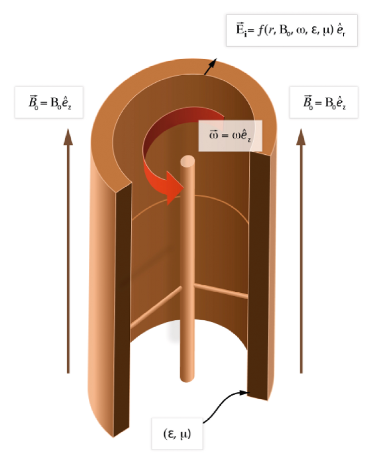
Figure 1: Details of the Wilson & Wilson Experiment. A magnetic insulator rotates with uniform angular velocity $\vec{\omega}=\omega\boldsymbol{\hat{e}}_{\mathtt{z}}$ in an external magnetic field
$\vec{B}_{\mathbf{o}}=\mathrm{B}_{\mathbf{o}}\boldsymbol{\hat{e}}_{\mathtt{z}}$. An electric field $\vec{E}_{\mathbf{i}}=f(r,\mathrm{B}_{\mathbf{o}},\omega,\mathbf{\varepsilon,\mu})\boldsymbol{\hat{e}}_{r}$ is observed.

We start by introducing some useful notation. First  we write the Minkowski metric $\boldsymbol{\mathring{g}}$ as

$$\boldsymbol{\mathring{g}=\eta}_{\mu\nu}\boldsymbol{\theta}^{\mu}\otimes\boldsymbol{\theta}^{\nu}$$ (135)

with

$$\boldsymbol{\theta}^{0}=dt,\text{ \ \ }\boldsymbol{\theta}^{1}=dr,\text{ \ \ \ }\boldsymbol{\theta}^{2}=rd\phi,\text{ \ \ }\boldsymbol{\theta}^{3}=dz.$$ (136)

For our problem the moving boundary of our material has equations $\Xi_{1}=r-r_{1}=0$  and $\Xi_{2}=r-r_{2}=0$, so the normal to this surface is $d\Xi=\boldsymbol{\theta}^{1}$. For our problem we  have $\mathbf{J}=0.$ To proceed we write as an ansatz the solution for the electromagnetic field in the interior of the material

$$F_{\mathbf{i}}=\mathcal{E}\boldsymbol{\theta}^{0}\wedge\boldsymbol{\theta}^{1}+\mathcal{B}\boldsymbol{\theta}^{1}\wedge\boldsymbol{\theta}^{2}$$ (137)

where $\mathcal{E}$ and $\mathcal{B}$ are supposed to be functions only on the coordinate $r$.

We recall from Eq.(89) that the $1$-form physically equivalent to the velocity field $\boldsymbol{V}$ is

$$\boldsymbol{v}=\gamma(\boldsymbol{\theta}^{0}+\mathtt{v}\boldsymbol{\theta}^{2})\text{ }$$

with $\mathtt{v}=\omega r$ and $\gamma=(1-\mathtt{v}^{2})^{-1/2}$. We now must solve the equation $d\star G=0$ with the boundary conditions given by Eqs.(118) and (119). To calculate $G_{\mathbf{i}}$ we use Eq.(69). First we calculate $\boldsymbol{v\lrcorner}F_{\mathbf{i}}$. We have

$$\boldsymbol{v\lrcorner}F_{\mathbf{i}} =\gamma(\boldsymbol{\theta}^{0}+\mathtt{v}\boldsymbol{\theta}^{2})\lrcorner(\mathcal{E}\boldsymbol{\theta}^{01}+\mathcal{B}\boldsymbol{\theta}^{12})$$

$$=\gamma(\mathcal{E}+\mathtt{v}\mathcal{B})\boldsymbol{\theta}^{1}.$$

and

$$\boldsymbol{v}\wedge(\boldsymbol{v\lrcorner}F_{\mathbf{i}})=\gamma^{2}(\mathcal{E}+\mathtt{v}\mathcal{B})\boldsymbol{\theta}^{01}-\gamma^{2}\mathtt{v}(\mathcal{E}+\mathtt{v}\mathcal{B})\boldsymbol{\theta}^{12}.$$

Then

$$G_{\mathbf{i}} =\frac{\mathcal{E(\mathbf{\mu\varepsilon}-}\mathtt{v}^{2})+\mathcal{B\mathtt{v}(\mathbf{\mu\varepsilon}-}1)}{\mathcal{\mathbf{\mu}}(1-\mathtt{v}^{2})}\boldsymbol{\theta}^{01}+\frac{\mathcal{E\mathtt{v}(}1\mathcal{-\mathbf{\mu\varepsilon}})+\mathcal{B}(1-\mathcal{\mathbf{\mu\varepsilon}}\mathtt{v}^{2})}{\mathcal{\mathbf{\mu}}(1-\mathtt{v}^{2})}\boldsymbol{\theta}^{12}$$

$$:=\mathcal{K}\boldsymbol{\theta}^{01}+\mathcal{L}\boldsymbol{\theta}^{12}.$$ (138)

Since

$$\star(\boldsymbol{\theta}^{0}\wedge\boldsymbol{\theta}^{1}) =\widetilde{(\boldsymbol{\theta}^{0}\wedge\boldsymbol{\theta}^{1})}\lrcorner\boldsymbol{\tau}_{\boldsymbol{\mathring{g}}}=-\boldsymbol{\theta}^{2}\wedge\boldsymbol{\theta}^{3},$$

$$\star(\boldsymbol{\theta}^{1}\wedge\boldsymbol{\theta}^{2}) =\widetilde{(\boldsymbol{\theta}^{1}\wedge\boldsymbol{\theta}^{2})}\lrcorner\boldsymbol{\tau}_{\boldsymbol{\mathring{g}}}=\boldsymbol{\theta}^{0}\wedge\boldsymbol{\theta}^{3}$$

we have

$$\star G_{\mathbf{i}}=-\mathcal{K}\boldsymbol{\theta}^{23}+\mathcal{L}\boldsymbol{\theta}^{03}.$$ (139)

Then $d\star G=0$ gives

$$-\frac{d\mathcal{K}}{dr}\boldsymbol{\theta}^{123}-\frac{\mathcal{K}}{r}\boldsymbol{\theta}^{123}-\frac{d\mathcal{L}}{dr}\boldsymbol{\theta}^{013}=0$$

and so our problem resumes in solving the following two trivial ordinary differential equations

$$\frac{d\mathcal{K}}{dr}+\frac{\mathcal{K}}{r}=0\text{ \ and \ }\frac{d\mathcal{L}}{dr}=0,$$ (140)

with solutions

$$\mathcal{K}=\frac{c_{1}}{r}\text{ \ and \ }\mathcal{L}=c_{2}$$ (141)

respectively, where $c_{1}$ and $c_{2}$ are integration constants. So, we have

$$G_{\mathbf{i}} =\frac{c_{1}}{r}\boldsymbol{\theta}^{01}+c_{2}\boldsymbol{\theta}^{12},$$

$$\star G_{\mathbf{i}} =-\frac{c_{1}}{r}\boldsymbol{\theta}^{23}+c_{2}\boldsymbol{\theta}^{03}.$$

Now, if we recall that outside the magnetic insulator we have $\star G_{\mathbf{o}}=\star F_{\mathbf{o}}=\mathrm{B}_{\mathbf{o}}\boldsymbol{\theta}^{03}$ we get using the jump condition Eq.(119) that

$$(\star G_{\mathbf{o}}-\star G_{\mathbf{i}})\wedge\boldsymbol{\theta}^{1}=0,$$ (142)

i.e.,

$$-\mathrm{B}_{\mathbf{o}}\boldsymbol{\theta}^{013}+c_{2}\boldsymbol{\theta}^{013}-\frac{c_{1}}{r}\boldsymbol{\theta}^{123}=0$$ (143)

from where it follows that the functions $\mathcal{K}$ and $\mathcal{L}$ are

$$\mathcal{K}=0\text{, \ \ }\mathcal{L}=\mathrm{B}_{\mathbf{o}}.$$ (144)

Then from Eq.(138) we have the following system of linear equations for the functions $\mathcal{E}$ and $\mathcal{B}$:

$$\left\{\begin{array}[c]{c}\mathcal{E(\mathbf{\mu\varepsilon}-}\mathtt{v}^{2})+\mathcal{B\mathtt{v}(\mathbf{\mu\varepsilon}-}1)=0,\\ \frac{\mathcal{E}\mathtt{v}\mathcal{(}1\mathcal{-\mathbf{\mu\varepsilon}})+\mathcal{B}(1-\mathcal{\mathbf{\mu\varepsilon}}\mathtt{v}^{2})}{\mathcal{\mathbf{\mu}}(1-\mathtt{v}^{2})}=\mathrm{B}_{\mathbf{o}}\end{array}\right.$$ (145)

whose solution is:

$$\mathcal{E}=\mathrm{B}_{\mathbf{o}}\frac{\omega r(1-\mathcal{\mathbf{\mu\varepsilon}})}{\mathcal{\mathbf{\varepsilon}}(1-\omega^{2}r^{2})},\text{ \ \ }\mathcal{B}=-\mathrm{B}_{\mathbf{o}}\frac{(\omega^{2}r^{2}-\mathcal{\mathbf{\mu\varepsilon}})}{\mathcal{\mathbf{\varepsilon}}(1-\omega^{2}r^{2})}.$$ (146)

So, finally we have

$$F_{\mathbf{i}}=\mathrm{B}_{\mathbf{o}}\frac{\omega r(1-\mathcal{\mathbf{\mu\varepsilon}})}{\mathcal{\mathbf{\varepsilon}}(1-\omega^{2}r^{2})}\boldsymbol{\theta}^{01}-\mathrm{B}_{\mathbf{o}}\frac{(\omega^{2}r^{2}-\mathcal{\mathbf{\mu\varepsilon}})}{\mathcal{\mathbf{\varepsilon}}(1-\omega^{2}r^{2})}\boldsymbol{\theta}^{12}.$$ (147)

and the electric and magnetic fields $\underset{\boldsymbol{l}}{\boldsymbol{E}_{\mathbf{i}}}$  and $\underset{\boldsymbol{l}}{\boldsymbol{H}_{\mathbf{i}}}$ as determined in the laboratory frame inside the material are

$$\underset{\boldsymbol{l}}{\boldsymbol{E}_{\mathbf{i}}} =\boldsymbol{\theta}^{0}\lrcorner F_{\mathbf{i}}=\mathrm{B}_{\mathbf{o}}\frac{\omega r(1-\mathcal{\mathbf{\mu\varepsilon}})}{\mathcal{\mathbf{\varepsilon}}(1-\omega^{2}r^{2})}\boldsymbol{\theta}^{1},$$ (148)

$$\underset{\boldsymbol{l}}{\boldsymbol{H}_{\mathbf{i}}} =\boldsymbol{\theta}^{0}\lrcorner\star F_{\mathbf{i}}=-\mathrm{B}_{\mathbf{o}}\frac{(\omega^{2}r^{2}-\mathcal{\mathbf{\mu\varepsilon}})}{\mathcal{\mathbf{\varepsilon}}(1-\omega^{2}r^{2})}\boldsymbol{\theta}^{3}.$$ (149)

From Eq.(148) it follows immediately that the potential $V$ between the internal and external parts of the material as shown in Figure 1 is, when $\omega^{2}r^{2}<<1,$

$$V =\mathrm{B}_{\mathbf{o}}\omega\frac{1}{\mathcal{\mathbf{\varepsilon}}}(1-\mathcal{\mathbf{\mu\varepsilon}}){\textstyle\int\nolimits_{r_{1}}^{r_{2}}}rdr$$

$$=\frac{1}{2}\mathrm{B}_{\mathbf{o}}\omega\frac{1}{\mathcal{\mathbf{\varepsilon}}}(1-\mathcal{\mathbf{\mu\varepsilon}})(r_{2}^{2}-r_{1}^{2}),$$ (150)

which is the value found by Wilson & Wilson [21].

Exercise 13

Calculate $\underset{\boldsymbol{l}}{\boldsymbol{P}}$, $\underset{\boldsymbol{l}}{\boldsymbol{M}}$, the bound current $\underset{\boldsymbol{l}}{\mathcal{J}}$ and the bound charge $\underset{\boldsymbol{l}}{\rho}$.

6 Extracting Energy from the Magnetic Field

We now propose a way to extract energy from a magnetic field using the results just obtained above. In order to do that we first recall that when the magnetic insulator in Figure 1 which has momentum of inertia $I$ is put in rotation with constant angular velocity $\vec{\omega}=\omega\boldsymbol{\hat{e}}_{\mathtt{z}}$ it acquires an angular momentum

$$\vec{L}_{mec}=I\vec{\omega}.$$ (151)

For the preliminaries theoretical considerations in this section we suppose that there are no energy losses due to friction of the rotating magnetic insulator with its supporters nor losses due to Joule effect on electric wires. As a consequence the  total angular momentum of the system (i.e., the rotating dielectric plus the electromagnetic field) must be conserved. We suppose moreover that the system does not dissipate energy through radiation. Under these conditions the total angular momentum of the system is

$$\vec{L}_{\mathbf{t}}=\vec{L}_{mec}+\vec{L}_{elec}$$ (152)

where by [12] Abraham’s formula

$$\vec{L}_{elec}={\textstyle\int}d\mathtt{x}d\mathtt{y}d\mathtt{z}\overset{\rightarrow}{\mathtt{x}}\times(\vec{E}_{\mathbf{i}}\times\vec{H}_{\mathbf{i}}).$$ (153)

We choose our coordinate system such that the origin lives in the middle of the rotating axis of the dielectric. Under these conditions

$$\vec{E}_{\mathbf{i}}\times\vec{H}_{\mathbf{i}} =-\mathrm{B}_{\mathbf{o}}^{2}\frac{\mathcal{\mathbf{\mu}}(1-\mathcal{\mathbf{\mu\varepsilon}})\omega r(\omega^{2}r^{2}-\mathcal{\mathbf{\mu\varepsilon}})}{\mathcal{\mathbf{\varepsilon}}^{2}(1-\omega^{2}r^{2})^{2}}\boldsymbol{\hat{e}}_{r}\times\hat{e}_{\mathtt{z}}$$

$$=f(r,\mathrm{B}_{\mathbf{o}},\omega,\mathcal{\mathbf{\mu}},\mathcal{\mathbf{\varepsilon}})\boldsymbol{\hat{e}}_{\phi}.$$

Then

$$\mathtt{\vec{x}}\times(\vec{E}_{\mathbf{i}}\times\vec{H}_{\mathbf{i}}) =(\mathtt{z}\boldsymbol{\hat{e}}_{\mathtt{z}}+r\boldsymbol{\hat{e}}_{r})\times f(r,\mathrm{B}_{\mathbf{o}},\omega,\mathcal{\mathbf{\mu}},\mathcal{\mathbf{\varepsilon}})\boldsymbol{\hat{e}}_{\phi}$$

$$=\mathtt{z}f(r,\mathrm{B}_{\mathbf{o}},\omega,\mathcal{\mathbf{\mu}},\mathcal{\mathbf{\varepsilon}})\boldsymbol{\hat{e}}_{\mathtt{z}}\times\boldsymbol{\hat{e}}_{\phi}+rf(r,\mathrm{B}_{\mathbf{o}},\omega,\mathcal{\mathbf{\mu}},\mathcal{\mathbf{\varepsilon}})\boldsymbol{\hat{e}}_{r}\times\boldsymbol{\hat{e}}_{\phi}$$

$$=-\mathtt{z}f(r,\mathrm{B}_{\mathbf{o}},\omega,\mathcal{\mathbf{\mu}},\mathcal{\mathbf{\varepsilon}})\boldsymbol{\hat{e}}_{r}+rf(r,\mathrm{B}_{\mathbf{o}},\omega,\mathcal{\mathbf{\mu}},\mathcal{\mathbf{\varepsilon}})\boldsymbol{\hat{e}}_{\mathtt{z}}$$

$$=-\mathtt{z}f(r,\mathrm{B}_{\mathbf{o}},\omega,\mathcal{\mathbf{\mu}},\mathcal{\mathbf{\varepsilon}})(\cos\phi\boldsymbol{\hat{e}}_{\mathtt{x}}+\sin\phi\boldsymbol{\hat{e}}_{\mathtt{y}})+rf(r,\mathrm{B}_{\mathbf{o}},\omega,\mathcal{\mathbf{\mu}},\mathcal{\mathbf{\varepsilon}})\boldsymbol{\hat{e}}_{\mathtt{z}}.$$

Thus the integral corresponding to the $\boldsymbol{e}_{r}$ component vanishes and we have

$$\vec{L}_{elec} =\boldsymbol{e}_{\mathtt{z}}{\textstyle\int}r^{2}f(r,\mathrm{B}_{\mathbf{o}},\omega,\mathcal{\mathbf{\mu}},\mathcal{\mathbf{\varepsilon}})drd\phi d\mathtt{z}$$

$$=2\pi Z\boldsymbol{e}_{\mathtt{z}}{\textstyle\int_{r^{1}}^{r_{2}}}r^{2}f(r,\mathrm{B}_{\mathbf{o}},\omega,\mathcal{\mathbf{\mu}},\mathcal{\mathbf{\varepsilon}})dr.$$ (154)

where $Z$ is the height of the cylindrical dielectric. When $\omega^{2}r^{2}<<1$

$$\vec{L}_{elec} =\boldsymbol{\hat{e}}_{\mathtt{z}}2\pi Z\frac{\mathcal{\mathbf{\mu}}^{2}}{\mathcal{\mathbf{\varepsilon}}}\mathrm{B}_{\mathbf{o}}^{2}\omega(1-\mathcal{\mathbf{\mu\varepsilon}}){\textstyle\int_{r^{1}}^{r_{2}}}r^{3}dr$$

$$=-\frac{\pi Z\mathcal{\mathbf{\mu}}^{2}}{2\mathcal{\mathbf{\varepsilon}}}\mathrm{B}_{\mathbf{o}}^{2}\omega(\mathcal{\mathbf{\mu\varepsilon-}}1)\left(r_{2}^{4}-r_{1}^{4}\right)\boldsymbol{\hat{e}}_{\mathtt{z}}.$$ (155)

It is a remarkable fact that $\vec{L}_{elec}$ points in the opposite direction of $\vec{L}_{mec}$ if $\mathcal{\mathbf{\mu\varepsilon>}}1$ (as it is the case in the Wilson & Wilson experiment according to [11]. Since the total angular momentum of our system must be conserved we see that $\left|\vec{L}_{mec}\right|$ must increase if there is no energy losses due to friction and Joule effect in the wires and we could use the potential $V$ given by Eq.(150) to power an electric machine. Of course the energy powering the electric machine can only be coming from the energy stocked in the external magnetic field. It will work while the external magnetic field is presented. Of course extracting energy from the magnetic field will make the value of $\mathrm{B}_{\mathbf{o}}$ to decrease and with this decrease the potential $V$ will also decrease and at the end the machine will stop working.

Remark 14

If $\mathcal{\mathbf{\mu\varepsilon<}}1$ the electromagnetic angular momentum is in the same direction of the mechanical angular momentum, which must start to decrease after the device is put in rotation. Then, the electric field will decrease also making the electromagnetic momentum to decrease whereas the mechanical angular momentum must then start to increase again. It is not clear at this moment if the system will oscillate between a minimum and maximal mechanical angular momentum or will stabilize.

Remark 15

Real World Machine. In the real world where friction and Joule effect are always present in order to extract energy from the magnetic field we need a machine like the one in Figure 2 where the potential difference $V$ given by Eq.(150) is used first, if necessary, to power in a compensator motor just enough to restore eventual losses due to friction and Joule effect on the electric wires, and secondly $V$ is also used to power a motor to generate useful work.

7 Conclusions

In this paper we recalled how to correctly solve Maxwell equations in order to find the electric field in the famous Wilson & Wilson experiment using the theory of differential forms with permits an intrinsic formulation of the problem. We present also the correct jump conditions for the $F$ and $G$ fields in an invariant way when the boundary separating two media is in motion. We give enough details for the paper to be useful for students and researchers. Moreover we use the theoretical results to present a surprising result which for the best of our knowledge is new: a machine that can extract energy from an external magnetic field. Under appropriate conditions ($\mathcal{\mathbf{\mu\varepsilon>}}1$) the machine once puts in motion will start increasing the electromagnetic angular momentum stocked in the electromagnetic field in the direction contrary to the original mechanical angular momentum of the device which thus will start increasing (theoretically) its angular speed until $\omega r_{2}=1$, thus generating a big potential even in a small external magnetic field which can be use to produce useful work.

Of course, a machine like this one if in orbit around a neutron star can produce a lot of energy in a simple way than the hypothetical machine described, e.g., in page 908 [9] projected to extract energy from black holes by throwing garbage on it.

Figure 2: Machine to Extract Energy from an External Magnetic Field.

Appendix A Some Useful Formulas

In this appendix we present some useful identities of the theory of differential forms with has been used several times in the main text.

For $a\in\sec{\textstyle\bigwedge\nolimits^{1}}T^{\ast}M$ and $A_{r}\in\sec{\textstyle\bigwedge\nolimits^{r}}T^{\ast}M,B_{r}\in\sec{\textstyle\bigwedge\nolimits^{s}}T^{\ast}M$ it is

$$a\lrcorner(A_{r}\wedge B_{r})=(a\lrcorner A_{r})\wedge B_{r}+\hat{A}_{r}\wedge(a\lrcorner B_{r}).$$ (156)

$$\begin{array}[c]{l}A_{r}\wedge\underset{\boldsymbol{g}}{\star}B_{s}=B_{s}\wedge\underset{\boldsymbol{g}}{\star}A_{r};\quad r=s\\ A_{r}\cdot\underset{\boldsymbol{g}}{\star}B_{s}=B_{s}\cdot\underset{\boldsymbol{g}}{\star}A_{r};\quad r+s=n\\ A_{r}\wedge\underset{\boldsymbol{g}}{\star}B_{s}=(-1)^{r(s-1)}\underset{\boldsymbol{g}}{\star}(\tilde{A}_{r}\lrcorner B_{s});\quad r\leq s\\ A_{r}\lrcorner\underset{\boldsymbol{g}}{\star}B_{s}=(-1)^{rs}\underset{\boldsymbol{g}}{\star}(\tilde{A}_{r}\wedge B_{s});\quad r+s\leq n\\ \underset{\boldsymbol{g}}{\star}A_{r}=\tilde{A}_{r}\lrcorner\tau_{\boldsymbol{g}}\\ \underset{\boldsymbol{g}}{\star}\tau_{\boldsymbol{g}}=\mathrm{sgn\det}\boldsymbol{g};\quad\underset{\boldsymbol{g}}{\star}1=\tau_{\boldsymbol{g}}.\end{array}$$ (157)

Acknowledgement Authors are grateful to Flavia Tonelli for the figures.

References

- [1] Canovan, C. E. S., and Tucker, R. W., Maxwell Equations in a Uniformly Rotating Dielectric Medium and the Wilson-Wilson Experiment. [arXiv:1104.0574v1 [math-phys]]
- [2] Jackson, J. D., Classical Electrodynamics (third edition), J. Wiley & Sons, New York, 1999.
- [3] Giglio, J. F. T., and Rodrigues, W. A. Jr., Locally Inertial Reference Frames in Lorentzian and Riemann-Cartan Spacetimes, Annalen der Physik 502, 302-310 (2012).
- [4] Graham, G. M , and Lahoz, D. G, Observation of Static Electromagnetic Angular Momentum in Vacuo, Nature 285, 154-155 (1980).
- [5] Hertzberg, J. B., Bickman, S. R., Hummon, M. T., Krause, D., Jr., Peck, S. K., and Hunter, L .R., Measurement of the Relativisitic Potential Difference Across a Rotating Magnetic Dielectric Cylinder, Am. J. Phys. 69, 648-654 (2001).
- [6] Hehl, F. W., and Obukhov, Y. N., Foundations of Classical Electrodynamics, Birkhäuser, Boston 2003.
- [7] Lahoz, D. G. and Graham, G. M ,Observation of Electromagnetic Angular Momentum within Magnetite, Phys. Rev. Lett. 42, 1137–1140 (1979).
- [8] Lovelock, D. and Rund, H., Tensors, Differential Forms, and Variational Principles, John Wiley & Sons, New York, 1975.
- [9] Misner, C. W., Thorne, K. S., and Wheeler, J. A., Gravitation, W. H. Freeman and Co., San Francisco 1973.
- [10] Namias, V., Discontinuity of Electromagnetic Fields, Potentials, and Currents at Fixed and Moving Boundaries, Am. J. Phys. 56, 898-904 (1998).
- [11] Pellegrini, G. N., and Swift, A. R., Maxwell Equations in a Rotating Medium: Is there a Problem? Am. J. Phys. 63, 694-705 (1995).
- [12] Ramos, T., Rubilar, G. F., and Obukhov, Y. N., Relativistic Analysis of the Dielectric Einstein Box: Abraham, Minkowski and Total Energy-Momentum Tensors, Phys. Lett. A. 375, 1703-1709 (2011).
- [13] Ridgely, C. T., Applying Relativistic Electrodynamics to a Rotating Material Medium, Am. J. Phys. 66, 114-121 (1998).
- [14] da Rocha, R., and Rodrigues, W. A. Jr., Pair and Impair, Even and Odd Form Fields and Electromagnetism, Annalen der Physik 19, 6-34 (2010).
- [15] Rodrigues, W. A. Jr., and Capelas de Oliveira, E., The Many Faces of Maxwell, Dirac and Einstein Equations. A Clifford Bundle Approach. Lecture Notes in Physics 722, Springer, Heidelberg, 2007.[Errata at http://www.ime.unicamp.br/~walrod/svf3a.pdf].
- [16] Rodrigues, F. G., On Equivalent Expressions for the Faraday’s Law of Induction, Rev. Bras. Ens. de Fis. 34, 1309 (2012).[arXiv:1002.2792v2 [physics.class-ph]]
- [17] Webster, D. L., Relativity of Moving Circuits and Magnets, Am J. Phys. 29, 262- 268 (1960).
- [18] Webster, D. L, Schiff’s Charges and Currents in Rotating Matter, Am J. Phys. 31, 590- 597 (1963).
- [19] Schiff, L. I. , A Question in General Relativity, Proc. Nat. Acad. Sci. 25, 391-395 (1939).
- [20] Shiozawa, T., Phenomenological and Electron-Theoretical Study of the Electrodynamics of Rotating Systems, Proc. of the IEEE 61, 1694-1702 (1973).
- [21] Wilson, M., and Wilson, H.A., On the Electric Effect of Rotating a Magnetic Insulator in a Magnetic Field, Proc. R. Soc. London Ser. A 89, 99-106 (1913).