Limit Distribution of Averages over Unstable Periodic Orbits Forming Chaotic Attractor

Abstract

We address the question of representativeness of a single long unstable periodic orbit for properties of the chaotic attractor it is embedded in. Y. Saiki and M. Yamada [Phys. Rev. E 79, 015201(R) (2009)] have recently suggested the hypothesis that there exist a limit distribution of averages over unstable periodic orbits with given number of loops, $N$, which is not a Dirac $\delta$-function for infinitely long orbits. In this paper we show that the limit distribution is actually a $\delta$-function and standard deviations decay as $N^{-1/2}$ for large enough $N$.

1 Introduction

Recent investigations Saiki-Yamada-2009 ; Kawahara-Kida-2001 ; Kato-Yamada-2003 ; vanVeen-Kidaa-Kawahara-2006 ; Nikitin-2007 have arose the question of representativeness of a single unstable periodic orbit (UPO) for properties of the chaotic attractor it is embedded in. Interestingly, while Refs. Kawahara-Kida-2001 ; Kato-Yamada-2003 ; vanVeen-Kidaa-Kawahara-2006 concern unstable time-periodic orbits in turbulence, Ref. Nikitin-2007 discusses turbulent pipe flows in relation to spatially periodic solutions. Motivated by Kawahara-Kida-2001 ; Kato-Yamada-2003 ; vanVeen-Kidaa-Kawahara-2006 ; Nikitin-2007 Y. Saiki and M. Yamada Saiki-Yamada-2009 discus the calculation of average values along UPOs (unstable periodic orbits embedded into the chaotic attractor) and using the results of such a calculation for estimation of averages along a chaotic trajectory. In particular, with simple paradigmatic chaotic systems—the Lorenz system, the Rössler one, and a 6-dimensional economic model—Y. Saiki and M. Yamada explored the convergence of average values calculated along UPOs as the number of loops, $N$, of a UPO grows. They surprisingly found that the distribution of average values along all the UPOs with given $N$ (henceforth, $N$-UPOs) practically does not shrink for long orbits ($N=10...14$ for the Lorenz system, $N=10...17$ for the Rössler one), suggesting the existence of a limit distribution of averages over $N$-UPOs, which is not a Dirac $\delta$-function for infinitely long orbits ($N\to\infty$). In Ref. Zaks-Goldobin-2010 , it was shown that the UPOs with the length $N\leq 14$ are not enough long for conclusions on asymptotic behavior.

We are interested in the asymptotic behavior of the distribution of average values over UPOs with fixed $N$. Notice, the evaluation of average values for the chaotic attractor requires this distribution to be weighted with the distribution of the natural measure over the set of UPOs; in Ref. Grebogi-Ott-Yorke-1988 the natural measure of an UPO was shown to be inverse proportional to its multiplier. Meanwhile, we restrict our consideration to the question of convergence of the limit distribution and do not consider the distribution of the natural measure.

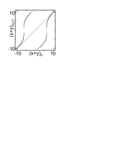
(a)   
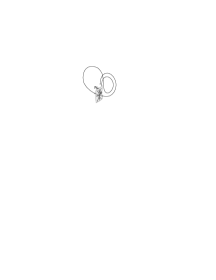
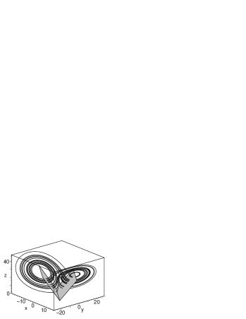
(b)     (c)

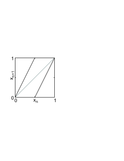
Figure 1: Chaos arising via bifurcations of homoclinic orbits. The phase portrait and the Poincaré section for the Lorenz system with classical parameter values (a). The Poincaré map for $(x+y)$ (b) is qualitatively similar to the saw map (c).

In this work we treat two maps: “saw” map

$$x_{n+1}=2x_{n}\mod{1}\,$$ (1)

—paradigmatic model for the chaos (i) arising via cascade of bifurcations of homoclinic orbits (as in the Lorenz system Lorenz-1963 , Fig. 1a) Kaplan-Yorke-1979 ; Lyubimov-Zaks-1983 —and “tent” map

$$x_{n+1}=\left\{\begin{array}[]{cc}2x_{n}&\mbox{for }x_{n}\leq 1/2\,,\\[10.0pt] 2-2x_{n}&\mbox{for }x_{n}>1/2\end{array}\right.$$ (2)

—paradigmatic model for the chaos (ii) arising via cascade of the period-doubling bifurcations (as in the Rössler system, Fig. 2a) Feigenbaum-1978 ; Feigenbaum-1979 ; Collet-Eckmann-Koch-1981 . The reason for our choice is not only paradigmaticity of these maps but also the fact that one gains exceptional technical opportunities for calculating all UPOs in them for giant $N$. We find the distributions of averages upon $N$-UPOs to shrink as $N$ grows; standard deviations decay as $1/\sqrt{N}$. Then we consider the Lorenz (the first sort of chaotic systems) and find for it the same kind dependence of standard deviations on $N$ as for the paradigmatic map models. Convergence of the distribution to a $\delta$-function can be observed for enough long UPOs (for the Lorenz system $N\geq 10$, cf. Fig. 4).

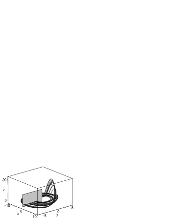
(a)     (b)

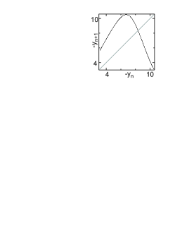
Figure 2: Chaos arising via cascade of the period-doubling bifurcations. The Poincaré section (a) and map (b) for the Rössler system with classical parameter values .

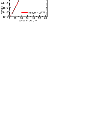
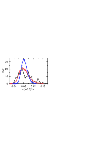
(a)     (b)
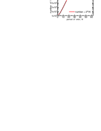
(c)     (d)
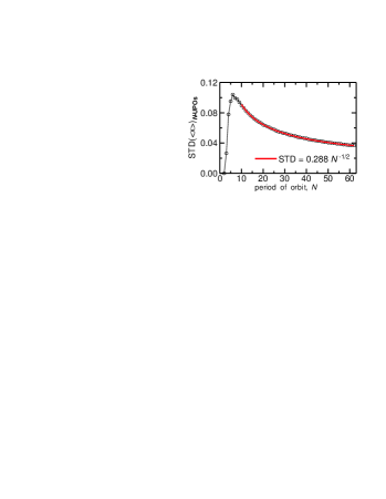
(e)     (f)

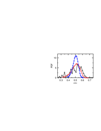
Figure 3: The number of UPOs used for averaging is presented by circles for the saw (a) and the tent (b) map; until the plateau, all UPOs are detected and employed, and on the plateau we utilize UPOs chosen randomly with a probability uniform over all $N$-UPOs. The standard deviations of $\langle(x-1/2)^{2}\rangle$ for the saw map (c) and the one of $\langle{x}\rangle$ for the tent map (d) decay as $1/\sqrt{N}$ for enough large $N$. The PDFs of the averages can be seen to shrink slowly as $N$ grows for both the saw (e) and the tent (f) maps; circles: $N=11$, squares: $N=23$, diamonds: $N=61$.

2 Limit Distribution of Averages

Let us first recall the origin of maps (1) and (2) in order to make the physical representativeness of these models evident. In the systems where the both separatrices of the saddle knot ${\bf P}$ come back in the vicinity of the stable manifold $W_{s}$ of ${\bf P}$ (Fig. 1a) the touching of a separatrix and $W_{s}$ results in appearance of the homoclinic orbit. The cascade of bifurcations of such orbits leads to the formation of the chaotic set (in the Lorenz system this cascade occurs at the single point $r\approx 13.927$ owing to the symmetry $(x,y)\leftrightarrow(-x,-y)$, cf. Lorenz-1963 ; Kaplan-Yorke-1979 ; Lyubimov-Zaks-1983 ). For the Lorenz system

$$\frac{dx}{dt}=\sigma(y-x)\,,$$

$$\frac{dy}{dt}=rx-y-xz\,,$$ (3)

$$\frac{dz}{dt}=-bz+xy$$

with the classical parameter set [$\sigma=10$, $b=8/3$, $r=28$] we choose $z=[(r-1)/(4b)]^{1/2}|x+y|$ as a Poincaré section, and find that the transversal structure of its intersection with the chaotic set is very narrow (Fig. 1); the Poinceré map for $(x+y)$ is visually unambiguous (Fig. 1b) and similar to the saw map (Fig. 1c). The averaging of a certain value along a certain trajectory on the chaotic set can be reduced to the averaging of a certain function $f(x+y)$ along the trajectory in the Poincaré map of $(x+y)$. The system symmetry suggests an even function $f(x+y)=f(-x-y)$. Actually, the contribution of $f(x+y)$ into $\langle{f(x+y)}\rangle$ over an orbit after one Poincaré recurrence is weighted by $T(x+y)/\langle{T(x+y)}\rangle_{\mathrm{map}}$, the ratio of the recurrence time for the trajectory running from $(x+y)$ and the average recurrence time for the orbit, $\langle...\rangle_{\mathrm{map}}$ stands for averaging over iterations of the Poincaré map (not over real time). Hence, $\langle{f(x+y)}\rangle=\langle{f(x+y)\,T(x+y)}\rangle_{\mathrm{map}}/\langle{T(x+y)}\rangle_{\mathrm{map}}$, i.e., $\langle{f(x+y)}\rangle$ is subject to the additional dispersion due to nonuniformity of $\langle{T(x+y)}\rangle_{\mathrm{map}}$ over various orbits. However, the nature of the dispersion of $\langle{T}\rangle_{\mathrm{map}}$ is the same as the one of $\langle{f\,T}\rangle_{\mathrm{map}}$, and in this paper we do not introduce any additional complication into our averagings with the paradigmatic map models. On the whole, the possibility to construct the Poincaré map in the vicinity of the saddle knot qualitatively similar to the saw map is the common peculiarity of the systems with a stable chaotic set of the kind we consider.

With regard to the second sort of chaotic systems, the existence of a unimodal map is a key feature needed for the cascade of the period-doubling bifurcations to occur resulting in chaotic behavior of the system Feigenbaum-1978 ; Feigenbaum-1979 ; Collet-Eckmann-Koch-1981 . Thus, for instance, the Poincaré map of the Rössler system (Fig. 2) is quite similar to parabola of the logistic map $x_{n+1}=bx_{n}(1-x_{n})$. The attracting chaotic set of the logistic map possesses its largest size at $b=4$ where this map can be turned into the tent one (2) by virtue of substitution $x\to\sin{\pi x}$. Hence, the tent map is quite representative for the systems where chaos arises via the cascade of the period-doubling bifurcations.

As it is noticed above, the symmetry of the Lorenz system suggests us consideration of $\langle{f(x)}\rangle$: $f(1/2+x)=f(1/2-x)$ along trajectories in the saw map. Hence, for simplicity, we consider $\langle(x-1/2)^{2}\rangle$ for the saw map (1) and $\langle{x}\rangle$ for the tent one (1). For the Lorenz system we calculate $\langle{x^{2}}\rangle$ and $\langle{z}\rangle$.

The dynamics of the saw map (1) can be easily dealt with within the frameworks of the binary notation of $x$. In this notation, an iteration of map (1) results in the shift of the binary point in $x$ by one position to the right and omitting the integer part. Thus, $x$ with an $N$-periodic sequence of digits in the binary mantissa belongs to an $N$-periodic orbit. Employing this fact one can strictly calculate giant amount of UPOs and averages along them. Dealing in such a fashion with the tent map (2) is less efficient and more sophisticated, but still possible. In Fig. 3 one can see that for enough large $N$ the standard deviations of the averages decay as $1/\sqrt{N}$. Additionally, for $\langle{x}\rangle$ in the saw map, which is actually beyond our immediate interest, one can analytically find probability $P(\langle{x}\rangle=m/N)\approx N!/[2^{N}m!(N-m)!]$, where $m=1,2,...,N-1$, and, for $N\gg 1$, $P(\langle{x}\rangle)\approx(2\pi N)^{-1/2}\exp(-2N\langle{x}\rangle^{2})$ and $\mathrm{STD}(\langle{x}\rangle)_{N-\mathrm{UPOs}}=(4N)^{-1/2}+O(N^{-1})$.

(a)     (b)

Figure 4: (a): STD normalized by STD for $N=15$ is plotted by circles for the saw map and by crosses for the Lorenz system [ $\mathrm{STD}(\langle{x^{2}}\rangle)_{15-\mathrm{UPOs}}\approx 0.5086323$ ] (b): The PDF of $\langle{x^{2}}\rangle$ for the Lorenz system shrinks only slightly as $N$ grows at the interval $[10,20]$. Solid line: $N=11$, dashed line: $N=15$, dash-dotted line: $N=19$.

In order to verify how far our findings for the paradigmatic map models are relevant for the chaotic systems with continuous time, UPOs in the Lorenz system (3) have been numerically calculated with double precision. We have calculated all UPOs with $N\leq 19$ (in Ref. Saiki-Yamada-2009 $90\%$ of UPOs with $N\leq 14$ were detected) and evaluated $\langle{x^{2}}\rangle$ and $\langle{z}\rangle$ along the detected UPOs. In Fig. 4 one can see the same scaling law for long UPOs; $\mathrm{STD}\propto N^{-1/2}$. The dependence of STD on $N$ for the Lorenz system and the saw map are similar for small $N$ as well (Fig. 4a).

Notice, the tendency of the PDF to shrinking as $N$ grows can be hardly detected from plots of PDFs (see Figs. 3e,f and 4b) for $N\in[10,20]$ which were typical for Ref. Saiki-Yamada-2009 .

3 Conclusion

Summarizing, we have analyzed two paradigmatic map models: the saw map (1) representing chaos arising via cascade of bifurcations of homoclinic orbits and the tent one (2) representing chaos arising via cascade of the period-doubling bifurcations. For the both models we have reliably established the fact that the distributions of averages along unstable periodic orbits with given number of loops $N$ shrinks to a Dirac $\delta$-function for $N\to\infty$; the standard deviations obey the decay law $N^{-1/2}$ for $N>10$. For the Lorenz system the same features have been confirmed. In particular, the average over a long UPO gives a correct representation of the average over the whole chaotic set which it is embedded in.

- (1) Collet, P., Eckmann, J.-P., Koch, H.: Period doubling bifurcations for families of maps on . J. Stat. Phys. 25, 1–14 (1981).
- (2) Feigenbaum, M.J.: Quantitative universality for a class of nonlinear transformations. J. Stat. Phys. 19, 25–52 (1978)
- (3) Feigenbaum, M.J.: The universal metric properties of nonlinear transformations. J. Stat. Phys. 21, 669–706 (1979)
- (4) Grebogi, C., Ott, E., Yorke, J.A.: Unstable Periodic Orbits and the Dimensions of Multifractal Chaotic Attractors. Phys. Rev. A 37, 1711–1724 (1988)
- (5) Kaplan, J.L., Yorke, J.A.: Preturbulence: A regime observed in a fluid flow model of Lorenz. Commun. Math. Phys. 67, 93–108 (1979)
- (6) Kato, S., Yamada, M.: Unstable periodic solutions embedded in a shell model turbulence. Phys. Rev. E 68, 025302(R) (2003)
- (7) Kawahara, G., Kida, S.: Periodic motion embedded in plane Couette turbulence: regeneration cycle and burst. J. Fluid Mech. 449, 291–300 (2001)
- (8) Lorenz, E.N.: Deterministic Nonperiodic Flow. J. Atmos. Sci. 20, 130–141 (1963)
- (9) Lyubimov, D.V., Zaks, M.A.: Two mechanisms of the transition to chaos in finite-dimensional models of convection. Physica 9D, 52–64 (1983)
- (10) Nikitin, N.: Spatial periodicity of spatially evolving turbulent flow caused by inflow boundary condition. Phys. Fluids 19, 091703 (2007)
- (11) Saiki, Y., Yamada, M.: Time-averaged properties of unstable periodic orbits and chaotic orbits in ordinary differential equation systems. Phys. Rev. E 79, 015201(R) (2009)
- (12) van Veen, L., Kidaa, S., Kawahara, G.: Periodic motion representing isotropic turbulence. Fluid Dyn. Res. 38, 19–46 (2006)
- (13) Zaks, M.A., Goldobin, D.S.: Comment on “Time-averaged properties of unstable periodic orbits and chaotic orbits in ordinary differential equation systems.” Phys. Rev. E 81, 018201 (2010)