Microlensing Evidence for Super-Eddington Disc Accretion in Quasars

Abstract

Microlensing by the stellar population of lensing galaxies provides an important opportunity to spatially resolve the accretion disc structure in strongly lensed quasars. Disc sizes estimated this way are on average larger than the predictions of the standard Shakura-Sunyaev accretion disk model. Analysing the observational data on microlensing variability allows to suggest that some fraction of lensed quasars (primarily, smaller-mass objects) are accreting in super-Eddington regime. Super-Eddington accretion leads to formation of an optically-thick envelope scattering the radiation formed in the disc. This makes the apparent disc size larger and practically independent of wavelength. In the framework of our model, it is possible to make self-consistent estimates of mass accretion rates and black hole masses for the cases when both amplification-corrected fluxes and radii are available.

1 Introduction

Since the work of Lynden-Bell (1969), disc accretion onto supermassive black holes is a commonly accepted interpretation for the activity of quasars, both radio-loud and radio-quiet (sometimes distinguished as quasi-stellar objects, QSO). Among all the active galactic nuclei, quasars are distinguished by higher luminosities (exceeding that of host galaxies) that is most likely connected to higher accretion rates.

Spectral energy distributions in optical and UV are reasonably consistent (Elvis et al., 1994) with the predictions of the standard thin accretion disc model introduced in the seminal works of Shakura (1972); Shakura & Sunyaev (1973); Lynden-Bell & Pringle (1974); Novikov & Thorne (1973). However, the predicted angular sizes of quasar accretion discs are too small (microarcseconds and less) to be resolved directly. For today, quasars remain essentially point-like (“quasi-stellar”) objects resolved only indirectly, in particular by microlensing effects.

As it was shown by Agol & Krolik (1999), microlensing by the stellar population of lensing galaxies is sensitive to the size of the emitting region. Here, we adopt the statement of Mortonson et al. (2005) that the basic quantity that microlensing amplification maps and curves are sensitive to is half-light radius. Half-light radius $R_{1/2}$ is defined as the radius inside which half of the observed flux is emitted at a given wavelength.

Numerous studies aimed on probing the spatial properties of quasar accretion discs with help of microlensing. While most early works (see Wambsganss (2006) for review) reported reasonable agreement between the observational data and the standard accretion disc theory, several important results are at odds with the theoretical predictions. Studying microlensing amplification statistics, Pooley et al. (2007) find best-fit disc sizes more than one order of magnitude larger than the theoretical predictions based on photometrical data. Partially, this may be attributed to the mass estimates used in this study (see discussion in Abolmasov & Shakura (2012)). In Morgan et al. (2010), inconsistency is somewhat smaller (about a factor of 3) but still significant. Accretion discs seem too large for their apparent luminosities or too faint for their sizes in the UV/optical range ($\sim 2000\mbox{\,--\,}4000\rm\AA$). Many papers (such as Jiménez-Vicente et al. (2012), Pooley et al. (2007) and Morgan et al. (2010)) interpret this inconsistency as an evidence for insufficiency of the standard accretion disc model, but no universal solution was proposed so far to account for the size discrepancy. There are indications for possibly higher black hole masses in some objects (Morgan et al., 2010; Abolmasov & Shakura, 2012), but no changes in masses, accretion rates and efficiencies can explain the observed sizes and fluxes simultaneously.

One of the important issues in quasar microlensing studies is whether the disc radial scale $R_{S}$ (Morgan et al., 2010) dependence on wavelength is consistent with the power law $R_{S}\propto\lambda^{4/3}$ predicted by the standard accretion disc theory. Several important disc models predict power law dependences $R(\lambda)\propto\lambda^{\zeta}$ with different exponents. Below we will refer to $\zeta$ as “structure parameter”. While for QSO J2237+0305, classical $\zeta=4/3$ works fairly good (Eigenbrod et al., 2008; Anguita et al., 2008), other objects such as SDSS 0924+0219, for instance, clearly require smaller $\zeta$. Floyd et al. (2009) propose angular momentum inflow at the inner edge of the disc in SDSS 0924+0219 (Agol & Krolik, 2000) as an explanation for the apparently very steep temperature law in the disc. This model implies $R_{S}\propto\lambda^{8/7}$ marginally consistent with the observational data.

In the recent work by Blackburne et al. (2011), several other objects were shown to have much shallower $R(\lambda)$ dependences, some consistent with $R_{S}=const$ for a broad range of comoving wavelengths, $0.1\mu\lesssim\lambda\lesssim 1\mu$. The only object having conventional thin-disc scaling is MG J0414+0534 that has the highest mass among the sample of 12 objects considered by Blackburne et al. (2011). All the smaller-mass ($M\lesssim 10^{9}\mathrm{M_{\odot}}$) black holes are characterised by $\zeta\sim 0\mbox{\,--\,}0.5$.

Microlensing effects in the X-ray range are more profound than in the optical (Pooley et al., 2007). Independently of the disc structure in the optical and UV ranges, X-ray properties are more or less similar for all the objects where microlensing effects were studied in the X-ray range (Chen et al., 2011; Dai et al., 2010; Morgan et al., 2012). Evidently, X-ray emission comes from somewhere inside the inner $\sim 10\times GM/c^{2}$ (Chen et al., 2012), and the exact mechanisms driving the formation of the X-ray continuum and lines are yet to be revealed.

Small structure parameters originate not only for very steep temperature slopes in multi-blackbody models. For instance, $\zeta=0$ is naturally reproduced if the brightness distribution does not depend on wavelength. This may be achieved if the accretion disc is surrounded by an envelope optically thick to Thomson scattering. Without affecting its spectral properties, scattering changes the spatial brightness distribution of the disc radiation. In general, accretion disc will increase its apparent radius and lose its intrinsic radius dependence on wavelength. A possible origin for such a scattering envelope is super-Eddington accretion that leads to formation of a Thomson-thick wind (Shakura & Sunyaev, 1973). Since there is observational evidence that some quasars accrete in supercritical regime, especially at larger redshifts (Collin et al., 2002), we consider this scenario quite plausible.

In the following section 2, we describe a simple scattering envelope model that we use to account for the spatial properties of microlensed quasars. It will be shown that such an envelope may result from super-Eddington accretion by a supermassive black hole. In section 3 and 4, we describe the observational data and interpret them in the framework of the scattering envelope model. In section 5, we consider the possible connection between the putative class of supercritical quasars, broad absorption line (BAL) quasars, and make conclusions in section 6.

2 Spherical envelope model

Though the issue of super-Eddington accretion is complicated, and different effects like photon trapping should be taken into account, the simple picture of supercritical accretion introduced by Shakura & Sunyaev (1973) is sufficient for our needs. This picture is supported by comprehensive numerical simulations (Ohsuga et al., 2005; Ohsuga & Mineshige, 2011).

2.1 Transition to supercritical regime

Radiation pressure is the principal feedback source for disc accretion. While for a spherically-symmetric source, both radiation pressure force and gravity scale $\propto R^{-2}$ with distance that leads to the universal Eddington luminosity limit, accretion disc geometry makes the situation more complicated because the source is no longer isotropic, and the forces are no longer collinear. For a thin disc, vertical gravity component grows with the vertical coordinate $z$ while the flux generated in the disc does not significantly depend on $z$ high enough in the atmosphere. Thin accretion disc supported by radiation pressure will have thickness determined by the equilibrium of the vertical components of the two forces.

$$\frac{\varkappa}{c}F=\frac{\varkappa}{c}\frac{3}{8\pi}\frac{GM\dot{M}}{R^{3}}\left(1-\sqrt{\frac{R_{in}}{R}}\right)=\frac{GM}{R^{3}}H$$

Here, $R$ is the radial coordinate, $R_{in}$ is the inner disc edge that for a black hole disc it is instructive to identify with the innermost stable orbit radius, $\varkappa\sim 0.4\rm cm^{2}g^{-1}$ is electron scattering opacity, $c$ is the speed of light, $G$ is gravitational constant, $M$ and $\dot{M}$ are the black hole mass and accretion rate. $H$ is accretion disc half-thickness that may be subsequently expressed as:

$$H=\frac{3}{8\pi}\frac{\varkappa\dot{M}}{c}\left(1-\sqrt{\frac{R_{in}}{R}}\right)=\frac{3}{2}\frac{GM}{c^{2}}\dot{m}\left(1-\sqrt{\frac{R_{in}}{R}}\right)$$

Here, we normalised the mass accretion rate as $\dot{M}=\dot{M}^{*}\dot{m}$,

$$\dot{M}^{*}=\frac{L_{Edd}}{c^{2}}=\frac{4\pi GM}{c\varkappa},$$ (1)

where $L_{Edd}=4\pi GMc/\varkappa$ is the Eddington luminosity. When the thickness of the radiation-supported disc becomes comparable to its radius, thin-disc approximation breaks down and the balance of forces is inevitably shifted: gravity scales as $(z^{2}+R^{2})^{-1}$, while the disc radiation decreases more slowly because at these distances accretion disc is still a strongly extended radiation source. Hence we assume the disc super-Eddington if its equilibrium half-thickness is $H\geq R$. This condition defines the spherisation radius in a non-relativistic regime but with a correction term that may play non-negligible role near the critical accretion rate. Let us introduce dimensionless radius $r=R/R_{in}$, where $R_{in}=x_{in}\times GM/c^{2}$ is the inner radius of the disc. Dimensionless inner radius $x_{in}$ varies between 1 (extreme Kerr case, corotating disc) and 9 (extreme Kerr, counter-rotation). Existence of a supercritical region in the disc requires existence of a root $r>1$ of the following equation:

$$\frac{r}{1-1/\sqrt{r}}=\frac{3}{2}\frac{\dot{m}}{x_{in}}$$ (2)

This equation may be reduced to a cubic equation for $\sqrt{r}$ having either two or no positive real roots, depending on the right-hand side. The minimum of the left hand side is always at $r_{cr}=9/4$. This implies the critical accretion rate of $\dot{m}_{cr}=4.5x_{in}$. The luminosity of a non-relativistic disc with this value of mass accretion rate is $L/L_{Edd}=\dot{m}_{cr}\eta\simeq 9/4$, where $\eta=L/\dot{M}c^{2}$ is accretion efficiency. This value may be thought of as the gain that disc geometry provides for the Eddington limit. Without the correction term, the critical accretion rate should be about an order of magnitude lower, $\dot{m}_{cr,0}=2x_{in}/3$. This justifies the attention we pay to the correction term. Still, the real transition to supercritical accretion may be much more complicated and influenced by relativistic effects and the exact physics of wind acceleration.

Spherisation radius for $\dot{m}>\dot{m}_{cr}$ may be found in a way that takes into account the correction term:

$$R_{sph}=\frac{3}{2}\frac{GM}{c^{2}}\dot{m}\times\psi^{2}(\dot{m}/x_{in})$$ (3)

Here, $\psi$ is the correction multiplier that accounts for the influence of the inner radius in the disc. It may be found as the largest root of the cubic equation for $\sqrt{r}$ that follows from (2). When accretion is supercritical ($\dot{m}>\dot{m}_{cr}=4.5x_{in}$), the cubic equation has three roots and its solution may be expressed using trigonometric functions (Nickalls, 1993). Solving the cubic equation yield the following expression for correction multiplier:

$$\psi(x)=\frac{2}{\sqrt{3}}\cos\left(\frac{1}{3}\arccos\left(-\frac{3}{\sqrt{2x}}\right)\right)$$ (4)

For $\dot{m}\gg 1$, $\psi(\dot{m}/x_{in})$ rapidly approaches $1$, hence:

$$R_{sph}\simeq\frac{3}{2}\dot{m}\times\frac{GM}{c^{2}},$$

that coincides with the classical definition of spherisation radius (Shakura & Sunyaev, 1973).

Formation of disc winds in supercritical accretion regime is supported by numerical simulations (Ohsuga et al., 2005; Okuda et al., 2005). If the radiation flux from the disc exceeds the local Eddington value, some part of its energy is converted to kinetic energy of the outflow. Terminal wind velocity $v_{w}$ may be estimated through Bernoulli integral:

$$\frac{v_{w}^{2}}{2}\simeq\frac{GM}{R}\times\left(\frac{L}{L_{Edd}}-1\right)$$

For example, setting the luminosity to the “disc Eddington limit” $L=\frac{9}{4}L_{Edd}$ implies $v_{w}=\sqrt{2.5GM/R_{w}}$ where $R_{w}$ is some effective radius where the outflow is formed. Since most of the matter is ejected from $R\sim R_{sph}$, we assume the terminal velocity of the wind is proportional to the escape velocity at the spherisation radius:

$$v_{w}=\beta\sqrt{2GM/R_{sph}},$$ (5)

were $\beta\sim 1$ is some additional dimensionless multiplier introduced to account for the uncertain details of wind acceleration and formation of the outflow.

2.2 Spherical envelope radius

Let us assume that the envelope is composed of a fully ionised spherically-symmetric wind expanding at a constant velocity. Continuity equation allows to connect electron density with the mass loss rate $\dot{M}_{w}=f_{w}\dot{m}\dot{M}^{*}$ and outflow velocity $v_{w}$ calculated according to equation (5).

$$\rho=\frac{\dot{M}_{w}}{4\pi R^{2}v_{w}}$$

Envelope size is defined by the radius where the radial optical depth toward the observer is unity.

$$\tau(R)=\int_{0}^{+\infty}\varkappa\rho(R)dR=\frac{f_{w}\varkappa\dot{M}}{4\pi cv_{w}R}$$

$$R_{1}=R(\tau=1)=\frac{f_{w}\varkappa\dot{M}}{4\pi v_{w}}$$

$$\frac{R_{1}c^{2}}{GM}=\sqrt{\frac{3}{8}}\frac{f_{w}}{\beta}\dot{m}^{3/2}\psi(\dot{m}/x_{in})$$ (6)

For a moderately super-Eddington accretor with $f_{w}\sim 1$, the size of the envelope becomes comparable and may even exceed the size of the accretion disc in the ultraviolet range. Such a scattering envelope has a radius practically independent of wavelength while the spectral properties of the scattered radiation remain more or less unchanged. The envelope is actually a pseudo-photosphere: it expands supersonically at a large, possibly mildly relativistic velocity of $v\sim\dot{m}^{-1/2}c$.

2.3 Apparent intensity distribution

Half-light radius is defined by the general relation that may be used for any radially-symmetric intensity distribution:

$$\frac{\int_{R_{in}}^{R_{1/2}}I(R)RdR}{\int_{R_{in}}^{+\infty}I(R)RdR}=\frac{1}{2}$$ (7)

For a standard thin non-relativistic accretion disc, monochromatic intensity scales with radius as:

$$I(R)\propto\frac{1}{\exp\left(\left(R/R_{S}\right)^{3/4}\left(1-\sqrt{\frac{R_{in}}{R}}\right)\right)-1},$$

where $R_{S}$ is the disc radial scale defined by condition $h\nu_{em}=kT(R_{S})$ without the correction factor. If $R_{in}\ll R_{1/2}$, to a high accuracy:

$$\begin{array}[]{l}R_{1/2}^{(disc)}\simeq 2.44R_{S}\simeq\\ \qquad{}\simeq 2.44\left(\frac{45\lambda_{em}^{4}GM\dot{M}}{16\pi^{6}hc^{2}}\right)^{1/3}=\\ \qquad{}=2.44\left(\frac{45c^{3}\lambda_{em}^{4}\dot{m}}{4\pi^{5}h\varkappa GM}\right)^{1/3}\frac{GM}{c^{2}}\\ \end{array}$$ (8)

Here, $\lambda_{em}$ is the comoving (quasar reference frame) wavelength of the observed radiation ($\nu_{em}=c/\lambda_{em}$ is corresponding frequency; observed wavelengths and frequencies are denoted as $\lambda_{obs}$ and $\nu_{obs}$), $h$ is Planck constant.

For a spherical envelope, brightness is nearly uniform in the centre and declines as a power law at large radii. We have taken the extended scattering atmosphere model described in Appendix A and calculated the intensity at infinity for different shooting parameter values coming to the overall conclusion that the half-light radius in this model is proportional to the photosphere radius and $R_{1/2}^{(envelope)}\simeq 1.06R_{1}$.

2.4 Disc radiation

Standard accretion disc temperature law may be written (neglecting the correction term important for the inner parts of the disc) as:

$$T(R)=\left(\frac{3}{2}\frac{G^{2}M^{2}}{\sigma\varkappa c}R^{-3}\dot{m}\right)^{1/4},$$

where $\sigma$ is Stephan-Boltzmann constant. Monochromatic flux is found as an integral over the picture plane:

$$F_{\nu}=\int I_{\nu}d\Omega=\frac{2\pi\cos i}{D^{2}\times(1+z)^{3}}\int I_{\nu}(R)RdR$$

We use angular size distance $D=D(z)$, and $i$ is disc inclination. Assuming the radiation generated in the disc has locally a blackbody spectrum leads to the following estimate for monochromatic flux valid far away from the high- and low energy cut-offs connected to the inner and the outer disc edges:

$$\begin{array}[]{l}F_{\nu}=8\pi\left(\frac{2}{3}\right)^{1/3}\Gamma(8/3)\zeta(8/3)\frac{k^{8/3}\nu_{obs}^{1/3}}{c^{8/3}h^{5/3}\varkappa^{2/3}\sigma^{2/3}}\times\\ \qquad{}\times(GM)^{4/3}\dot{m}^{2/3}\cos i\times\frac{1}{D^{2}\times(1+z)^{8/3}}\\ \end{array}$$ (9)

Here, $\Gamma$ and $\zeta$ are Gamma-function and Riemann zeta-function (not to be confused with the structure parameter $\zeta$ that is used without any argument). The above formula may be used to estimate the mass of the supermassive black hole (SMBH) using one observable quantity (flux) and one unknown parameter $\dot{m}$.

$$\begin{array}[]{l}M=\left(\frac{3}{2}\right)^{1/4}\times(8\pi\Gamma(8/3)\zeta(8/3))^{-3/4}\times\frac{c^{2}h^{5/4}\varkappa^{1/2}\sigma_{B}^{1/2}}{Gk^{2}\nu_{obs}^{1/4}}\times\\ \qquad{}\times F_{\nu}^{3/4}\dot{m}^{-1/2}\cos^{-3/4}iD^{3/2}(z)\times(1+z)^{2}\end{array}$$ (10)

Spherical envelope scrambles the radiation generated in the disc and makes it roughly isotropic. Effective inclination cosine in this case is $\cos i_{eff}=1/2$ since the initially anisotropic flux $F_{\nu}\propto\cos i$ is re-distributed isotropically with the total luminosity conserved.

2.5 Mass and accretion rate estimates

Microlensing studies are unique for distant quasars since they allow to estimate the size of the emitting region in continuum independently of the observed flux. In the case of a standard accretion disc both observables, $F_{\nu}$ and $R_{1/2}$, may be used to estimate only one combination of black hole mass and accretion rate, $M^{2}\dot{m}$ (see also discussion in Abolmasov & Shakura (2012)). Existence of a scattering envelope allows to break this degeneracy and make self-consistent estimates of both principal parameters ($M$ and $\dot{m}$).

Solving the system of two equations (10) and (6) for $M$ and $\dot{m}$ allows to estimate both black hole mass and dimensionless accretion rate. We also set $\cos i=\cos i_{eff}=1/2$:

$$\begin{array}[]{l}\dot{m}=\frac{\sqrt{2}}{3^{3/4}}\left(8\pi\Gamma(8/3)\zeta(8/3)\right)^{3/4}\frac{k^{2}\nu_{obs}^{1/4}}{h^{5/4}\varkappa^{1/2}\sigma_{B}^{1/2}}\times\\ \qquad{}\times F_{\nu}^{-3/4}D^{-3/2}(z)(1+z)^{-2}\times\frac{\beta}{f_{w}}\frac{R_{1}}{\psi(\dot{m}/x_{in})}\simeq\\ \qquad{}\simeq 169\left(\frac{\lambda_{obs}}{0.79\mu}\right)^{-1/4}\times 10^{0.3(I-19)}\times\left(\frac{D}{1\mathrm{Gpc}}\right)^{-3/2}\times\\ \qquad{}\times(1+z)^{-2}\times\frac{\beta}{f_{w}}\frac{R_{1}}{10^{15}\rm cm}\frac{1}{\psi(\dot{m}/x_{in})}\\ \end{array}$$ (11)

Here, we expressed the observed flux through the magnitude $I$ in the HST F814W band ($\lambda_{obs}\simeq 0.79\mu$) adopting the zero-point flux equal to $F_{\nu}=2.475\times 10^{-20}\mathrm{erg\,cm^{-2}\,s^{-1}\,Hz^{-1}}$ (Holtzman et al., 1995) since we use the amplification-corrected magnitudes from Morgan et al. (2010) obtained in this photometrical band at the HST.

Since the left-hand side of (11) dependence on the mass accretion rate is much stronger, simple forward iteration works good. Once $\dot{m}$ is found, the black hole mass may be estimated following (10) as:

$$M\simeq 4.6\times 10^{7}\times 10^{-0.3(I-19)}\left(\frac{D(z)}{1\mathrm{Gpc}}\right)^{3/2}(1+z)^{2}\dot{m}^{-1/2}\mathrm{M_{\odot}}$$

2.6 Disc and envelope sizes

Depending on the wavelength range, a supercritical disc may be either observed directly (if its size is larger than the photosphere of the wind) or covered by the photosphere of the supercritical wind. Equality of the half-light radii set by the two radial scales leads to the following condition for observational importance of the envelope:

$$R_{1/2}^{(disc)}=R_{1/2}^{(envelope)}$$

$$2.44R_{S}=1.06R_{1}$$

After substituting equations (8) and (6), one gets the following mass limit:

$$\begin{array}[]{l}M_{lim}=\left(\frac{2.44}{1.06}\right)^{3}\left(\frac{4}{3}\right)^{3/2}\frac{45}{4\pi^{5}}\left(\frac{\beta}{f_{w}}\right)^{3}\times\\ \qquad{}\times\frac{c^{3}}{\varkappa hG}\lambda_{em}^{4}\dot{m}^{-7/2}\psi^{-3}(\dot{m}/x_{in})\simeq\\ \qquad{}\simeq 3.8\times 10^{10}\left(\frac{\lambda_{em}}{0.25\mu}\right)^{4}\left(\frac{\dot{m}}{10}\right)^{-7/2}\psi^{-3}(\dot{m}/x_{in})\mathrm{M_{\odot}}\end{array}$$ (12)

For higher masses (at a given wavelength, for fixed $\dot{m}$), the size of the envelope is smaller than the half-light radius of the disc, and the appearance of the quasar will be close to the thin disc case. The limit is shown in figures 1 and 2 with solid lines. This limit evidently depends on wavelength. For the sample of Morgan et al. (2010), comoving frame wavelength changes in the range $0.2\mbox{\,--\,}0.5\mu$ that corresponds to about a factor of 2 upward shift of the limit in figure 1.

3 Multi-wavelength data

3.1 Disc radii and amplification-corrected fluxes

We make use of the amplification-corrected fluxes and microlensing-based radii collected and published by Morgan et al. (2010). The sample of Morgan et al. (2010) overlaps with this of Blackburne et al. (2011). In the original work, disc radii are given in terms of accretion disc radial scale $R_{S}$. Since we propose that at least for some objects, emitting region has different nature and intensity distribution, we recalculate these disc radii into model-independent half-light radii. Fitted with a standard-disc model with radial scale $R_{S}$ as defined above, emitting region may be characterised by the half-light radius of $R_{1/2}\simeq 2.44R_{S}$. The scattering envelope model we use has one characteristic radius $R_{1}$ where optical depth equals unity. For this model, $R_{1/2}\simeq 1.06R_{1}$ (see Appendix A). Half-light radii are given in table 2. For all the objects studied by Morgan et al. (2010) and Blackburne et al. (2011), the two estimates are consistent within the uncertainties. Since the uncertainties are very high, it is difficult to set any constraints upon the possible variations of the half-light radii.

Table 1: Properties of the microlensed quasars from the sample of Morgan et al. (2010). Black hole mass $M_{S}$ and accretion rate $\dot{m}$ are calculated for the case of supercritical accretion for $a=0.9$.

Object	$M_{vir},10^{9}\mathrm{M_{\odot}}$	$I_{corr},mag$	$R_{1/2}$, $10^{15}\rm cm$	$R_{1/2}$, $10^{15}\rm cm$	$M_{S},10^{9}\mathrm{M_{\odot}}$	$\dot{m}$
			(Morgan et al., 2010)	(Blackburne et al., 2011)
HE J0435-1223	0.50	20.76$\pm$0.25	$12.23_{-26.44}^{+9.79}$	$9_{-5}^{+12}$	$0.028^{+0.03}_{-0.013}$	$70^{+90}_{-40}$
SDSS 0924+0219	0.11	21.24$\pm$0.25	$2.44_{-2.43}^{+1.47}$	$4.6_{-2.4}^{+5}$	$0.026^{+0.017}_{-0.009}$	$32^{+20}_{-15}$
FB J0951+2635	0.89	17.16$\pm$0.11	$30.72_{-46.44}^{+18.49}$	–	$0.33^{+0.15}_{-0.11}$	$31^{+30}_{-14}$
SDSS J1004+4112	0.39	20.97$\pm$0.44	$1.94_{-1.93}^{+0.97}$	–	$0.044^{+0.02}_{-0.015}$	$22^{+15}_{-8}$
HE J1104-1805	2.37	18.17$\pm$0.31	$19.38_{-11.34}^{+9.67}$	–	$0.42^{+0.25}_{-0.14}$	$23^{+12}_{-9}$
PG 1115+080	1.23	19.52$\pm$0.27	$97.14_{-96.68}^{+58.47}$	$52_{-27}^{+60}$	$0.047^{+0.02}_{-0.012}$	$140^{+110}_{-70}$
RXJ 1131-1231	0.06	20.73$\pm$0.11	$4.87_{-2.85}^{+1.80}$	$2.4_{-1.4}^{+3.6}$	$0.007^{+0.005}_{-0.003}$	$82^{+50}_{-30}$
SDSS J1138+0314	0.04	21.97$\pm$0.19	$1.94_{-5.78}^{+1.45}$	$8.9_{-5.9}^{+17}$	$0.03^{+0.03}_{-0.014}$	$27^{+30}_{-17}$
SBS J1520+530	0.88	18.92$\pm$0.13	$12.23_{-7.15}^{+4.51}$	–	$0.17^{+0.05}_{-0.04}$	$28^{+7}_{-6}$
QSO J2237+0305	0.9	17.90$\pm$0.44	$9.71_{-9.67}^{+4.85}$	–	$0.40^{+0.22}_{-0.14}$	$17^{+4}_{-3}$
Q J0158-4325	0.16	19.09$\pm$0.12	$1.94_{-1.93}^{+0.97}$	–	$0.168^{+0.05}_{-0.04}$	$10^{+10}_{-3}$
Q J0158-4325 (Morgan et al., 2012)	0.16	19.09$\pm$0.12	$10^{+20}_{-5}$	–	$0.07^{+0.04}_{-0.02}$	$50^{+30}_{-30}$

For their sample of objects, Morgan et al. (2010) also provide magnitudes corrected for strong lensing amplification (see also table 2) based upon HST observations in the F814W filter. Flux calibration is based on the paper of Holtzman et al. (1995), see section 2.5.

3.2 Masses and emissivity slopes

Several methods are used to estimate masses of supermassive black holes. Most of them are model-dependent and suffer from biases of different nature. For bright distant quasars, masses are usually estimated either through photometrical data (bolometric luminosity is restored from multi-wavelength observations) or by measuring the widths of broad emission lines and the size of the emitting region by reverberation mapping (Blandford & McKee, 1982). While the first method relies heavily on ad hoc assumptions about the mass accretion rate and accretion efficiency, the second has a fundamental uncertainty connected to the geometry of the emitting region. Virial mass is estimated as:

$$M=f\frac{\sigma^{2}R_{BLR}}{G},$$

where $\sigma^{2}$ is the velocity dispersion corresponding to the observed line width, $R_{BLR}$ is the size of the emitting region (determined with help of reverberation mapping), and coefficient $f$ is calibrated using better-studied nearby active galaxies where $f\simeq 5.5$ (Onken et al., 2004). Sometimes only a limited number of spectra is available and reverberation analysis in impossible. In this case, empirical virial relations (Vestergaard & Peterson, 2006) are used. These two types of mass estimates will be hereafter referred to as virial. Since we use the microlensing-based disc radii from Morgan et al. (2010) we also make use of the virial masses given in this work (see references in this paper, especially Peng et al. (2006)).

4 Results

4.1 Masses and accretion rates

Mass and dimensionless mass accretion rates estimated from the observables by the method introduced in section 2.5 are given in table 2 (for $a=0.9$ and $x_{in}=2.32$) and shown in figures 1 and 2 for two values of $a$ and $x_{in}$. All the masses and mass accretion rates were determined in the assumption of existence of an optically-thick scattering envelope. They apply only to the objects where the disc is surrounded by an envelope larger than the disc itself (i. e. above both the dotted and the solid lines in figure 1).

Figure 1: Quasar parameters (mass and dimensionless mass accretion rate) recovered in the framework of supercritical envelope. The left and the right panels correspond to $a=0$ ($x_{in}=6$) and $a=0.9$ ($x_{in}\simeq 2.32$), respectively. Horizontal dotted line shows the actual Eddington limit: accretion is sub-critical below the line and super-critical above it. Solid inclined line marks the limit where the envelope becomes larger than the disc monochromatic size (for $\lambda_{em}=0.25\mu$). Hereafter, thick dots show objects that are also present in the sample of Blackburne et al. (2011), and the recent result for Q J0158-4325 (Morgan et al., 2012) is shown by a star. Errors correspond to $1\sigma$ uncertainties in flux and radius.

Figure 2: Same as previous figure, but instead of dimensionless mass accretion rate $\dot{m}$, dimensional mass accretion rate $\dot{M}$ is given.

Errors given in table  and figures 1 and 2 were calculated using direct non-linear error propagation. We used the 1$\sigma$ uncertainties given by Morgan et al. (2010) for the radii and fluxes. Since we do not know the exact probability distributions of these quantities, it seems to be the most reasonable approach. We substituted $R_{1}\pm\Delta R_{1}$ and $I\pm\Delta I$ into equations (11) and (10) and interpreted the highest and the lowest values of $\dot{m}$ and $M$ as the ends of some representative confidence interval.

Properties of the larger part of the objects shown in figure 1 are consistent with accretion in a moderately super-Eddington regime. If the accretion efficiency is high ($a\gtrsim 0.9$), all the objects may be interpreted as super-Eddington. Most of the objects are however difficult to identify as super- or sub-Eddington sources due to large uncertainties in $\dot{m}$. More probable super-Eddington objects such as RXJ 1131-1231 and PG 1115+080 tend also to have lower $\zeta$ (see section 4.2). Einstein’s cross, one of the most probable sub-critical discs from the sample, is evidently among the lowest-$\dot{m}$ objects. According to our model, Q J0158-4325 should best conform to the thin disc model. Indeed, disc size for this object reported in Morgan et al. (2010) is in good agreement with the theoretical predictions. However, the recent work of Morgan et al. (2012) reports evidence for a larger disc size, several times larger than (but still consistent at about $1.5\sigma$ confidence level) the standard model predictions based on the measured amplification-corrected flux. Since dimensionless mass accretion rate is proportional to the envelope radius, the larger radius makes the properties of Q J0158-4325 consistent with our supercritical disc model.

Masses determined in the spherical envelope model are generally smaller than virial masses (see figure 3). Indeed, applicability of the classical virial relations to an expanding supercritical wind is questionable. As we will show in the section 5, the broad emission lines observed in quasar spectra are unlikely to be formed in the outflowing matter, but one still may expect violations of the virial relations derived for sub-critical active galactic nuclei.

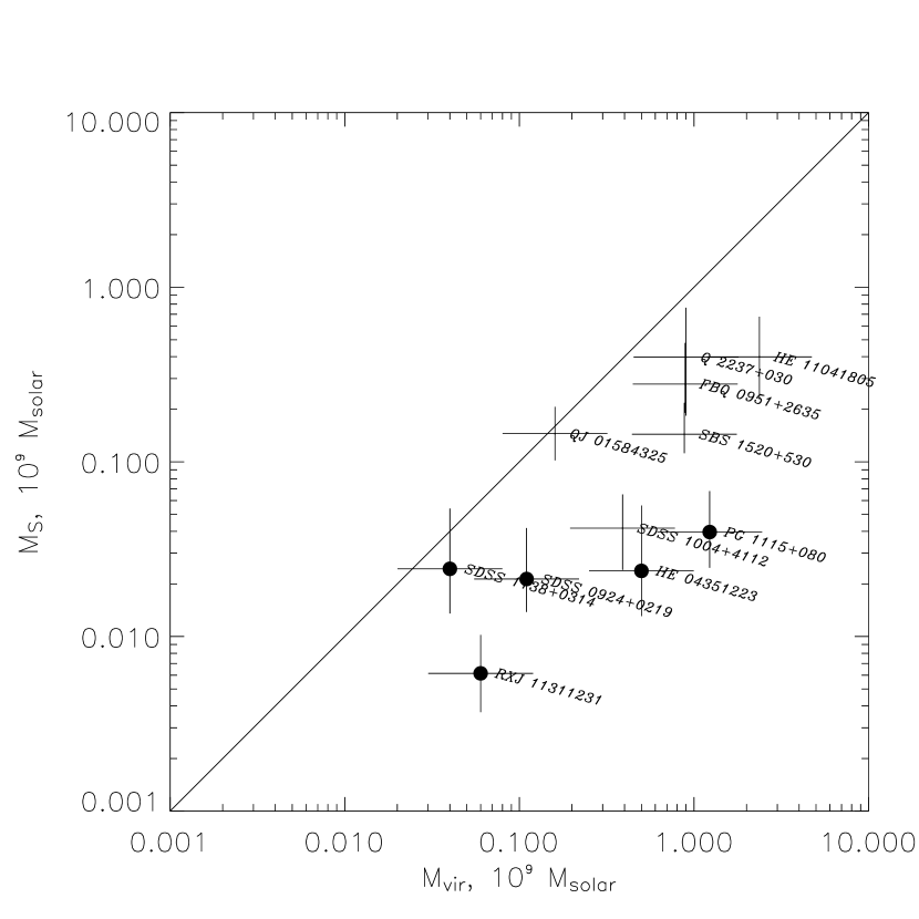
Figure 3: Virial masses plotted versus mass estimates in supercritical wind assumption . Kerr parameter was set to $a=0.9$.

4.2 Structure parameter correlation with mass

Several quasar microlensing studies used multi-wavelength data to trace the disc size dependence on wavelength. Fitting this dependence with a power law allows to check the validity of several accretion disc models such as thin disc ($\zeta=4/3$), slim or irradiated disc ($\zeta=2$) and a thin disc with a strong torque at the inner radius ($\zeta=8/7$). Available data are collected in table 2 and in figure 4.

Interestingly enough, all the objects where standard disc slope works have masses $M\gtrsim 10^{9}\mathrm{M_{\odot}}$. All the smaller-mass black holes show intensity distributions with much lower $\zeta$. Besides the large fitting errors, objects in figure 4 may be separated in two groups: high-mass black holes surrounded by accretion discs similar to standard and lower-mass objects where $\zeta\sim 0\mbox{\,--\,}0.5$. An evident qualitative solution is to propose that at least some quasars accrete in super-Eddington regime. If all the bright lensed quasars accrete at $\dot{M}\sim 30\mathrm{M_{\odot}\,yr^{-1}}$, Eddington luminosity will be reached for $M\sim 10^{9}\mathrm{M_{\odot}}$ for accretion efficiency $\eta\sim 0.1$. Lower-mass objects are expected to enter super-Eddington accretion phase easier and lose excess accreting matter (Shakura & Sunyaev, 1973). We propose that supercritical wind does not affect the spectral energy distributions of QSO much but changes its spatial properties, acting as a lampshade that changes only the visible size and shape of the lamp.

Table 2: Structure parameter as a function of SMBH mass. All the data were taken from Blackburne et al. (2011), if not stated otherwise.

Object	$M_{vir},$	$\zeta$	reference
	$10^{9}\mathrm{M_{\odot}}$
MG J0414+0534	$1.82$	$1.5\pm 0.8$
MG J0414+0534	$1.82$	$1.5\pm 0.5$	Bate et al. (2008)
HE J0435-1223	$0.50$	$0.7\pm 0.6$
RXJ 0911+0551	$0.80$	$0.17\pm 0.4$
SDSS 0924+0219	$0.11$	$0.17\pm 0.5$
SDSS 0924+0219	$0.11$	$0.7\pm 0.4$	Floyd et al. (2009)
HE J1104-1805	$2.37$	$1.65\pm 0.5$	Poindexter et al. (2008)
PG 1115+080	$1.05$	$0.4\pm 0.5$
RXJ 1131-1231	$0.06$	$0.4\pm 0.5$
SDSS J1138+0314	$0.04$	$0.4\pm 0.5$
QSO J2237+0305	$0.90$	$1.2\pm 0.3$	Eigenbrod et al. (2008)
QSO J2237+0305	$0.90$	$1.1\pm 0.3$	Eigenbrod et al. (2008)
			(no velocity prior)
QSO J2237+0305	$0.90$	$1.2^{+2}_{-0.6}$	Anguita et al. (2008)

Figure 4: Structure parameters for quasars of different masses. Virial masses are shown by crosses. For several objects(HE J0435-1223, SDSS 0924+0219, HE J1104-1805, PG 1115+080, RXJ 1131-1231, SDSS J1138+0314, QSO J2237+0305), we use our envelope model to estimate masses (shown by stars).

5 Discussion

In previous sections we have shown that some lensed quasars are surrounded by scattering envelopes of moderate optical depths $\tau\sim R_{1}/R_{sph}\sim\dot{m}^{1/2}\sim 1\mbox{\,--\,}10$. Expected outflow velocities are $v\sim\dot{m}^{-1/2}c$. At the same time, Doppler widths of broad emission lines are significantly lower, $v/c\sim 0.01$. Besides, the expected emission line luminosities are several orders of magnitude less than that of observed broad emission lines in quasars. If we propose a constant filling factor $f$, a recombination line in a supercritical outflow should have a luminosity estimated as the following volume integral:

$$L_{line}=\frac{1}{f}\alpha h\nu\times\int_{V}n_{e}n_{i}dV$$

Here, $\alpha$ is the recombination coefficient, $n_{e}$ and $n_{i}$ are the electron concentration and concentration of the particular ion emitting the line. It is convenient to express the concentrations as $n_{i}=n_{e}x_{i}=\rho x_{i}/m$. Below, we fix the values of $x_{i}$ and the effective particle mass $m$. For completely ionised hydrogen-rich gas, $m$ is about the proton mass.

$$\frac{L_{line}}{L_{Edd}}\simeq 10^{-7}\frac{f_{w}^{2}x_{i}\dot{m}^{2}}{f\beta^{2}}\frac{\alpha}{10^{-13}\rm cm^{3}s^{-1}}\frac{1000\rm\AA}{\lambda_{line}}\frac{R_{sph}}{R_{in}}$$

Integration is performed from some inner radius $R_{in}$ to infinity. Since the inner parts of the flow are considerably ionised the above luminosity is an upper estimate. Predicted equivalent widths are of the order $\sim 10^{-4}\rm\AA$, about five-six orders lower than the observed equivalent widths of broad emission lines. Conditions are much more favourable for formation of absorption lines, since the wind is thick to electron scattering and $N_{H}\sim\tau/m_{p}\sim 10^{24}\dot{m}^{1/2}\rm cm^{-2}$.

Outflows are expected to manifest themselves in blueshifted absorptions and P Cyg lines. Broad absorption line (BAL) quasars (Turnshek, 1984) show strongly blueshifted absorption components of UV and sometimes X-ray spectral lines. Two of the objects of our sample, PG 1115+080 and SBS J1520+530, are known as BAL quasars. PG 1115+080 also demonstrates signatures of moderately-relativistic outflows. In particular, Chartas et al. (2003) find two relativistic absorption components (at $\sim 0.1$ and $\sim 0.3c$) of highly ionised iron species and an OVI absorption component at $\sim 0.02c$. Similar X-ray absorption systems were found for some other high-redshift luminous quasars like APM 08279+5255 (Chartas et al., 2002), HE J1414+117 (Chartas et al., 2007) and HS 1700+6416 (Lanzuisi et al., 2012). Absorption components with relativistic velocities were also found in the UV spectra of some BAL, “mini-BAL” and narrow-absorption line quasars (see Narayanan et al. (2004) and references therein). Relativistic outflows often coexist with slower absorption systems, and UV and X-ray absorption lines usually show different profiles and velocities.

Discrepancy in wind velocities for different absorption components suggests that the wind is highly inhomogeneous, with different components having different velocities. Besides, its structure may be far from spherical symmetry, and even in the spherically-symmetric case the shape of the visible photosphere is distorted if the wind is relativistic (Abramowicz et al., 1991). For relativistic winds, there are two effects important for their spatial properties: (i) firstly, relativistic beaming makes the visible size of the emitting region $\sim\gamma^{3}$ times smaller, where $\gamma$ is Lorentz-factor, and (ii) secondly, the optical depth along the wind flow direction is smaller. Both effects are expected to produce a wavelength-dependent limb-darkening effect that may be responsible for deviations of $\zeta$ from 0 for some objects.

For several objects, the size of the X-ray emitting region was studied using microlensing effects (see Pooley et al. (2007); Chen et al. (2011, 2012); Morgan et al. (2012) and references therein). Independently of the UV/optical structure parameter $\zeta$, the X-ray sizes of all the studied quasars are estimated as several gravitational radii, that is sometimes one-two orders of magnitude smaller than the proposed envelope size. This is difficult to account for in the spherical envelope model since the size of the envelope (as well as the size of the accretion disc in the optical/UV range) is generally much larger.

However, the outflows formed by super-Eddington accretion discs are expected to possess high net angular momentum that leads to formation of an avoidance cone also known as supercritical funnel (Shakura & Sunyaev, 1973). This picture is supported by numerical simulations (Ohsuga et al., 2005; Okuda et al., 2005): for a large range of inclinations, the angular size of the source in X-rays is considerably smaller than the size of the outer photosphere of the wind. Optical depth of an envelope with a funnel is expected to be much lower (if the disc is viewed at low inclinations, see Poutanen et al. (2007)) for the innermost parts of the disc where the X-ray component is supposed to be formed. The non-monotonic optical depth dependence on radius predicted for supercritical accretion disc winds can qualitatively explain the decrease in the disc size at smaller wavelengths observed for some objects with $\zeta\sim 0$ such as PG 1115+080 and WF1 J2033-4723 (Blackburne et al., 2011).

As long as we use virial masses, properties of the X-ray radiation indicate that it is formed near the last stable orbit (Morgan et al., 2012). However, smaller masses recovered in the framework of our supercritical envelope model shift the last stable orbit toward lower sizes. For instance, the X-ray emitting region of RXJ 1131-1231 has the size of $\sim 2\times 10^{14}\rm cm$ (Dai et al., 2010). For the virial mass estimate of $6\times 10^{7}\mathrm{M_{\odot}}$, this corresponds to $\sim 7\times GM/c^{2}$, while the envelope-based mass is about an order of magnitude larger, and the estimated X-ray size becomes several tens of $GM/c^{2}$. This difference can hardly be used to distinguish between the individual mass estimates or individual models of X-ray emission separately. However, it should be borne in mind that virial masses are consistent with the models where X-ray emission is formed near the last stable orbit while the envelope-based mass estimates allow the X-ray emission to be extended for tens of gravitational radii. This is consistent, for example, with the models like Liu et al. (2012) where the X-rays are produced by the hot gas of the corona present in the inner parts of the accretion flow. In any case, the size of the X-ray emitting region is expected to be considerably smaller than both the disc size at $\sim 2500\rm\AA$ and the scattering wind photosphere size.

Existence of true absorption processes should also affect the apparent size of the spherical envelope. Assuming total thermalisation in a spherical relativistic wind, Fukue & Iino (2010) find that the visible photosphere surface follows the law $T(R)\propto R^{-1}$ that implies $\zeta\simeq 1$. More elaborate studies taking into account the temperature and ionisation structure of the wind are needed to explain the observed $\zeta\sim 0\mbox{\,--\,}0.5$ values of most of the putative supercritical quasars.

True absorption processes are also important for wind acceleration. In the super-Eddington regime, wind is efficiently launched by resonance lines even in presence of strong X-ray radiation (Proga et al., 2000; Proga & Kallman, 2004). Resonance lines do not alter the measured photosphere size significantly since the wind is opaque to absorption only in a narrow wavelength range. However, their contribution to wind acceleration through $\beta$ and $f_{w}$ may be important.

It is tempting to compare the population of super-Eddington quasars to the few known and well-studied supercritical black hole X-ray binaries, primarily to SS433 (Fabrika, 2004; Cherepashchuk, A. M. and Sunyaev, R. A. and Fabrika, S. N. et al., 2005). For SS433, dimensionless mass accretion rate is of the order several thousands that implies much slower outflow velocity of $\sim 1000\mathrm{km\,s^{-1}}$ and thermalised emission from the wind pseudo-photosphere. On the other hand, mass accretion rates estimated in the present work, as well as the values given by Collin et al. (2002), are considerably smaller. Maximal values are of the order $\dot{m}\sim 100\mbox{\,--\,}200$. Note that these values are only moderately supercritical, Eddington luminosity is exceeded a factor of $\sim 10\mbox{\,--\,}20$ (depending on the unknown accretion efficiency $\eta\sim 0.06\mbox{\,--\,}0.4$). It is more instructive to compare the population of super-Eddington quasars to the high-luminosity states of X-ray binaries like GRS J1915+105 (Vierdayanti et al., 2010) rather than to persistent strongly supercritical accretors like SS433 or to sources like V4641 (Revnivtsev et al., 2002) suffering strongly super-Eddington outbursts.

6 Conclusions

Scattering envelope formed by a super-Eddington accretion disc is a plausible model for the spatial properties of the emitting regions in some lensed quasars. Large spatial sizes ($R\sim 10^{16}\mbox{\,--\,}10^{17}\rm cm$) practically independent on wavelength are an expected outcome of a moderately super-Eddington ($\dot{m}\sim 10\mbox{\,--\,}100$) mass accretion rate. Black hole masses and mass accretion rates may be determined self-consistently if both disc size and flux estimates are present.

The small sizes of X-ray emitting regions of microlensed quasars may be explained by existence of an avoidance cone, or supercritical funnel, in the disc wind.

Some of our super-Eddington objects are broad absorption line quasars, and at least one (PG 1115+080) shows signatures of a mildly relativistic outflow.

Appendix A Brightness profile model

A.1 Radiation transfer in Eddington approximation

Optically-thick wind forms an extended pseudo-photosphere with a power-law density slope, $\rho\propto R^{-2}$. In general, radiation transfer is described by equation (Mihalas, 1978):

$$\mu\frac{\partial}{\partial R}\left(I\right)+\frac{1-\mu^{2}}{R}\frac{\partial}{\partial\mu}\left(I\right)=-\varkappa\rho(R)(S-I)$$

Here, $I=I(R,\mu)$ is monochromatic intensity, $\mu=\cos\theta$ is the cosine of the angle between the radius vector and radiation propagation direction, $S=S(R)$ is source function. We consider only isotropic coherent scattering that allows to equate source function to intensity averaged over solid angle. We use moment approach, and use the first three radiation intensity moments defined as:

$$J=\frac{1}{2}\int_{-1}^{+1}Id\mu$$ (13)

$$H=\frac{1}{2}\int_{-1}^{+1}I\mu d\mu$$ (14)

$$K=\frac{1}{2}\int_{-1}^{+1}I\mu^{2}d\mu$$ (15)

Figure 5: Principal scheme illustrating integration along the line of sight performed in the Appendix.

First radiation moment $J$ has the physical meaning of mean intensity, hence $S=J$ in our approximation. The system of moment equations is closed by Eddington’s assumption $K=fJ$ where $f=1/3$ valid in diffusion approximation. Questionability of Eddington approximation for extended atmospheres is well known Chapman (1966) but it is still sufficient for our purposes. Here, we consider pure electron scattering by a spherical atmosphere with electron density $n\propto\rho\propto R^{-2}$. In this case, the system of moment equations takes the form:

$$\left\{\begin{array}[]{l}\frac{1}{R^{2}}\frac{d}{dR}\left(R^{2}H\right)=0\\ \frac{d}{dR}\left(fJ\right)+\frac{3f-1}{R}J=-\varkappa\rho H\\ \end{array}\right.$$ (16)

The system is simplified if $f=1/3$ (inner parts, $\tau\gg 1$) and if $f=1$ (opposite limit, $\tau\to 0$). Mean intensity (and hence source function) scales in these two approximations as $\propto C_{1}R^{-3}$ and $\propto C_{2}R^{-2}\times(1+\tau)$, respectively. It is convenient to use the second formula and to set $C_{1}=C_{2}=H_{0}=H(\tau=1)$. Both asymptotics are then naturally reproduced. $H_{0}$ may be connected to the physical flux at the photosphere as $F(\tau=1)=4\pi H_{0}$ and luminosity as $L=(4\pi)^{2}R_{1}^{2}H_{0}$. However, this approximate formula does not conserve the total flux (intensity integrated over the solid angle deviates from the total radiation flux calculated as $F(\tau=1)=4\pi H_{0}$) that may result in systematic errors, hence we adopt the following form for the source function:

$$S(r)=H_{0}r^{-2}\times\left(1+d\times r^{-1/2}+r^{-1}\right),$$

where $r=R/R_{1}=1/\tau$, and $d$ is a free parameter. Integrating source function for some shooting parameter $P$ yields the observed intensity:

$$I=\varkappa\int_{-\infty}^{+\infty}S\left(\sqrt{P^{2}+l^{2}}\right)e^{-\tau(P,l)}\rho\left(\sqrt{P^{2}+l^{2}}\right)dl,$$

where $\tau(P,l)$ is the optical depth along the current line of sight:

$$\begin{array}[]{l}\tau=\varkappa\int_{-\infty}^{l}\rho\left(\sqrt{P^{2}+l^{2}}\right)dl=\\ =\frac{R_{1}}{P}\left({\rm atan\,}\frac{l}{P}+\pi/2\right)\end{array}$$

The coordinates and designations are shown in figure 5.

Finally, intensity distribution may be expressed as the following definite integral:

$$\begin{array}[]{l}I(p)=H_{0}\times\left(u_{2}(p)+u_{3}(p)+d\times u_{5/2}(p)\right)\end{array}$$ (17)

where $x=l/R_{1}$ and $p=P/R_{1}$, and:

$$u_{k}(p)=p^{-(k+1)}\int_{0}^{\pi}e^{-\theta/p}\sin^{k}\theta d\theta$$

Constant $d$ is tuned in a way to fit the integral flux value, $2\pi\int_{0}^{+\infty}I(p)pdp=4\pi H_{0}$. Numerical integration allows to estimate the value of $d\simeq-0.097$.

Half-light radius for this model may be estimated as $R_{1/2}=1.063R_{1}$ to an accuracy of about $10^{-3}$. Setting $d=0$ is also a reasonable approximation: it overestimates the flux by only about 5%, while $R_{1/2}\simeq 1.05R_{1}$ in this assumption.

References

- Abolmasov & Shakura (2012) Abolmasov P., Shakura N. I., 2012, MNRAS, 423, 676
- Abramowicz et al. (1991) Abramowicz M. A., Novikov I. D., Paczynski B., 1991, ApJ, 369, 175
- Agol & Krolik (1999) Agol E., Krolik J., 1999, ApJ, 524, 49
- Agol & Krolik (2000) Agol E., Krolik J. H., 2000, ApJ, 528, 161
- Anguita et al. (2008) Anguita T., Schmidt R. W., Turner E. L., Wambsganss J., Webster R. L., Loomis K. A., Long D., McMillan R., 2008, A&A, 480, 327
- Bate et al. (2008) Bate N. F., Floyd D. J. E., Webster R. L., Wyithe J. S. B., 2008, MNRAS, 391, 1955
- Blackburne et al. (2011) Blackburne J. A., Pooley D., Rappaport S., Schechter P. L., 2011, ApJ, 729, 34
- Blandford & McKee (1982) Blandford R. D., McKee C. F., 1982, ApJ, 255, 419
- Chapman (1966) Chapman R. D., 1966, ApJ, 143, 61
- Chartas et al. (2003) Chartas G., Brandt W. N., Gallagher S. C., 2003, ApJ, 595, 85
- Chartas et al. (2002) Chartas G., Brandt W. N., Gallagher S. C., Garmire G. P., 2002, ApJ, 579, 169
- Chartas et al. (2007) Chartas G., Eracleous M., Dai X., Agol E., Gallagher S., 2007, ApJ, 661, 678
- Chen et al. (2011) Chen B., Dai X., Kochanek C. S., Chartas G., Blackburne J. A., Kozłowski S., 2011, ApJL, 740, L34
- Chen et al. (2012) Chen B., Dai X., Kochanek C. S., Chartas G., Blackburne J. A., Morgan C. W., 2012, ApJ, 755, 24
- Cherepashchuk, A. M. and Sunyaev, R. A. and Fabrika, S. N. et al. (2005) Cherepashchuk, A. M. and Sunyaev, R. A. and Fabrika, S. N. et al. 2005, A&A, 437, 561
- Collin et al. (2002) Collin S., Boisson C., Mouchet M., Dumont A.-M., Coupé S., Porquet D., Rokaki E., 2002, A&A, 388, 771
- Dai et al. (2010) Dai X., Kochanek C. S., Chartas G., Kozłowski S., Morgan C. W., Garmire G., Agol E., 2010, ApJ, 709, 278
- Eigenbrod et al. (2008) Eigenbrod A., Courbin F., Meylan G., Agol E., Anguita T., Schmidt R. W., Wambsganss J., 2008, A&A, 490, 933
- Elvis et al. (1994) Elvis M., Wilkes B. J., McDowell J. C., Green R. F., Bechtold J., Willner S. P., Oey M. S., Polomski E., Cutri R., 1994, ApJSS, 95, 1
- Fabrika (2004) Fabrika S., 2004, Astrophysics and Space Physics Reviews, v.12, p.1-152 (2004) (http://www.cambridgescientificpublishers.com/), 12, 1
- Floyd et al. (2009) Floyd D. J. E., Bate N. F., Webster R. L., 2009, MNRAS, 398, 233
- Fukue & Iino (2010) Fukue J., Iino E., 2010, PASJ, 62, 1399
- Holtzman et al. (1995) Holtzman J. A., Burrows C. J., Casertano S., Hester J. J., Trauger J. T., Watson A. M., Worthey G., 1995, PASP, 107, 1065
- Jiménez-Vicente et al. (2012) Jiménez-Vicente J., Mediavilla E., Muñoz J. A., Kochanek C. S., 2012, ApJ, 751, 106
- Lanzuisi et al. (2012) Lanzuisi G., Giustini M., Cappi M., Dadina M., Malaguti G., Vignali C., Chartas G., 2012, A&A, 544, A2
- Liu et al. (2012) Liu J. Y., Liu B. F., Qiao E. L., Mineshige S., 2012, ApJ, 754, 81
- Lynden-Bell (1969) Lynden-Bell D., 1969, Nature, 223, 690
- Lynden-Bell & Pringle (1974) Lynden-Bell D., Pringle J. E., 1974, MNRAS, 168, 603
- Mihalas (1978) Mihalas D., 1978, Stellar atmospheres /2nd edition/. San Francisco, W. H. Freeman and Co., 1978. 650 p.
- Morgan et al. (2012) Morgan C. W., Hainline L. J., Chen B., Tewes M., Kochanek C. S., Dai X., Kozlowski S., Blackburne J. A., Mosquera A. M., Chartas G., Courbin F., Meylan G., 2012, ApJ, 756, 52
- Morgan et al. (2010) Morgan C. W., Kochanek C. S., Morgan N. D., Falco E. E., 2010, ApJ, 712, 1129
- Mortonson et al. (2005) Mortonson M. J., Schechter P. L., Wambsganss J., 2005, ApJ, 628, 594
- Narayanan et al. (2004) Narayanan D., Hamann F., Barlow T., Burbidge E. M., Cohen R. D., Junkkarinen V., Lyons R., 2004, ApJ, 601, 715
- Nickalls (1993) Nickalls R. W. D., 1993, Mathematical Gazette, 77, 354
- Novikov & Thorne (1973) Novikov I. D., Thorne K. S., 1973, in Black Holes (Les Astres Occlus) Astrophysics of black holes.. Gordon and Breach, Paris, pp 343–450
- Ohsuga & Mineshige (2011) Ohsuga K., Mineshige S., 2011, ApJ, 736, 2
- Ohsuga et al. (2005) Ohsuga K., Mori M., Nakamoto T., Mineshige S., 2005, ApJ, 628, 368
- Okuda et al. (2005) Okuda T., Teresi V., Toscano E., Molteni D., 2005, MNRAS, 357, 295
- Onken et al. (2004) Onken C. A., Ferrarese L., Merritt D., Peterson B. M., Pogge R. W., Vestergaard M., Wandel A., 2004, ApJ, 615, 645
- Peng et al. (2006) Peng C. Y., Impey C. D., Rix H.-W., Kochanek C. S., Keeton C. R., Falco E. E., Lehár J., McLeod B. A., 2006, ApJ, 649, 616
- Poindexter et al. (2008) Poindexter S., Morgan N., Kochanek C. S., 2008, ApJ, 673, 34
- Pooley et al. (2007) Pooley D., Blackburne J. A., Rappaport S., Schechter P. L., 2007, ApJ, 661, 19
- Poutanen et al. (2007) Poutanen J., Lipunova G., Fabrika S., Butkevich A. G., Abolmasov P., 2007, MNRAS, 377, 1187
- Proga & Kallman (2004) Proga D., Kallman T. R., 2004, ApJ, 616, 688
- Proga et al. (2000) Proga D., Stone J. M., Kallman T. R., 2000, ApJ, 543, 686
- Revnivtsev et al. (2002) Revnivtsev M., Gilfanov M., Churazov E., Sunyaev R., 2002, A&A, 391, 1013
- Shakura (1972) Shakura N. I., 1972, AZh, 49, 921
- Shakura & Sunyaev (1973) Shakura N. I., Sunyaev R. A., 1973, A&A, 24, 337
- Turnshek (1984) Turnshek D. A., 1984, ApJ, 280, 51
- Vestergaard & Peterson (2006) Vestergaard M., Peterson B. M., 2006, ApJ, 641, 689
- Vierdayanti et al. (2010) Vierdayanti K., Mineshige S., Ueda Y., 2010, PASJ, 62, 239
- Wambsganss (2006) Wambsganss J., 2006, in G. Meylan, P. Jetzer, P. North, P. Schneider, C. S. Kochanek, & J. Wambsganss ed., Saas-Fee Advanced Course 33: Gravitational Lensing: Strong, Weak and Micro Part 4: Gravitational microlensing. pp 453–540