The Rapid Atmospheric Monitoring System of the
Pierre Auger Observatory
Abstract
The Pierre Auger Observatory is a facility built to detect air showers produced by cosmic rays above eV. During clear nights with a low illuminated moon fraction, the UV fluorescence light produced by air showers is recorded by optical telescopes at the Observatory. To correct the observations for variations in atmospheric conditions, atmospheric monitoring is performed at regular intervals ranging from several minutes (for cloud identification) to several hours (for aerosol conditions) to several days (for vertical profiles of temperature, pressure, and humidity). In 2009, the monitoring program was upgraded to allow for additional targeted measurements of atmospheric conditions shortly after the detection of air showers of special interest, e. g., showers produced by very high-energy cosmic rays or showers with atypical longitudinal profiles. The former events are of particular importance for the determination of the energy scale of the Observatory, and the latter are characteristic of unusual air shower physics or exotic primary particle types. The purpose of targeted (or “rapid”) monitoring is to improve the resolution of the atmospheric measurements for such events. In this paper, we report on the implementation of the rapid monitoring program and its current status. The rapid monitoring data have been analyzed and applied to the reconstruction of air showers of high interest, and indicate that the air fluorescence measurements affected by clouds and aerosols are effectively corrected using measurements from the regular atmospheric monitoring program. We find that the rapid monitoring program has potential for supporting dedicated physics analyses beyond the standard event reconstruction.
keywords:
Cosmic rays, extensive air showers, air fluorescence method, atmospheric monitoring, calibration, radiosonde, lidar, star monitoringThe Pierre Auger Collaboration
P. Abreu63,
M. Aglietta51,
M. Ahlers94,
E.J. Ahn81,
I.F.M. Albuquerque15,
D. Allard29,
I. Allekotte1,
J. Allen85,
P. Allison87,
A. Almela11, 7,
J. Alvarez Castillo56,
J. Alvarez-Muñiz73,
R. Alves Batista16,
M. Ambrosio45,
A. Aminaei57,
L. Anchordoqui95,
S. Andringa63,
T. Antiči’c23,
C. Aramo45,
E. Arganda4, 70,
F. Arqueros70,
H. Asorey1,
P. Assis63,
J. Aublin31,
M. Ave37,
M. Avenier32,
G. Avila10,
A.M. Badescu66,
M. Balzer36,
K.B. Barber12,
A.F. Barbosa,
R. Bardenet30,
S.L.C. Barroso18,
B. Baughman,
J. Bäuml35,
C. Baus37,
J.J. Beatty87,
K.H. Becker34,
A. Bellétoile33,
J.A. Bellido12,
S. BenZvi94,
C. Berat32,
X. Bertou1,
P.L. Biermann38,
P. Billoir31,
F. Blanco70,
M. Blanco31, 71,
C. Bleve34,
H. Blümer37, 35,
M. Boháčová25,
D. Boncioli46,
C. Bonifazi21, 31,
R. Bonino51,
N. Borodai61,
J. Brack79,
I. Brancus64,
P. Brogueira63,
W.C. Brown80,
R. Bruijn,
P. Buchholz41,
A. Bueno72,
L. Buroker95,
R.E. Burton77,
K.S. Caballero-Mora88,
B. Caccianiga44,
L. Caramete38,
R. Caruso47,
A. Castellina51,
O. Catalano50,
G. Cataldi49,
L. Cazon63,
R. Cester48,
J. Chauvin32,
S.H. Cheng88,
A. Chiavassa51,
J.A. Chinellato16,
J. Chirinos Diaz84,
J. Chudoba25,
M. Cilmo45,
R.W. Clay12,
G. Cocciolo49,
L. Collica44,
M.R. Coluccia49,
R. Conceição63,
F. Contreras9,
H. Cook75,
M.J. Cooper12,
J. Coppens57, 59,
A. Cordier30,
S. Coutu88,
C.E. Covault77,
A. Creusot29,
A. Criss88,
J. Cronin90,
A. Curutiu38,
S. Dagoret-Campagne30,
R. Dallier33,
B. Daniel16,
S. Dasso5, 3,
K. Daumiller35,
B.R. Dawson12,
R.M. de Almeida22,
M. De Domenico47,
C. De Donato56,
S.J. de Jong57, 59,
G. De La Vega8,
W.J.M. de Mello Junior16,
J.R.T. de Mello Neto21,
I. De Mitri49,
V. de Souza14,
K.D. de Vries58,
L. del Peral71,
M. del Río46, 9,
O. Deligny28,
H. Dembinski37,
N. Dhital84,
C. Di Giulio46, 43,
M.L. Díaz Castro13,
P.N. Diep96,
F. Diogo63,
C. Dobrigkeit 16,
W. Docters58,
J.C. D’Olivo56,
P.N. Dong96, 28,
A. Dorofeev79,
J.C. dos Anjos13,
M.T. Dova4,
D. D’Urso45,
I. Dutan38,
J. Ebr25,
R. Engel35,
M. Erdmann39,
C.O. Escobar81, 16,
J. Espadanal63,
A. Etchegoyen7, 11,
P. Facal San Luis90,
H. Falcke57, 60, 59,
K. Fang90,
G. Farrar85,
A.C. Fauth16,
N. Fazzini81,
A.P. Ferguson77,
B. Fick84,
J.M. Figueira7,
A. Filevich7,
A. Filipčič67, 68,
S. Fliescher39,
C.E. Fracchiolla79,
E.D. Fraenkel58,
O. Fratu66,
U. Fröhlich41,
B. Fuchs37,
R. Gaior31,
R.F. Gamarra7,
S. Gambetta42,
B. García8,
S.T. Garcia Roca73,
D. Garcia-Gamez30,
D. Garcia-Pinto70,
G. Garilli47,
A. Gascon Bravo72,
H. Gemmeke36,
P.L. Ghia31,
M. Giller62,
J. Gitto8,
H. Glass81,
M.S. Gold93,
G. Golup1,
F. Gomez Albarracin4,
M. Gómez Berisso1,
P.F. Gómez Vitale10,
P. Gonçalves63,
J.G. Gonzalez35,
B. Gookin79,
A. Gorgi51,
P. Gouffon15,
E. Grashorn87,
S. Grebe57, 59,
N. Griffith87,
A.F. Grillo52,
Y. Guardincerri3,
F. Guarino45,
G.P. Guedes17,
P. Hansen4,
D. Harari1,
T.A. Harrison12,
J.L. Harton79,
A. Haungs35,
T. Hebbeker39,
D. Heck35,
A.E. Herve12,
C. Hojvat81,
N. Hollon90,
V.C. Holmes12,
P. Homola61,
J.R. Hörandel57, 59,
P. Horvath26,
M. Hrabovský26, 25,
D. Huber37,
T. Huege35,
A. Insolia47,
F. Ionita90,
A. Italiano47,
S. Jansen57, 59,
C. Jarne4,
S. Jiraskova57,
M. Josebachuili7,
K. Kadija23,
K.H. Kampert34,
P. Karhan24,
P. Kasper81,
I. Katkov37,
B. Kégl30,
B. Keilhauer35,
A. Keivani83,
J.L. Kelley57,
E. Kemp16,
R.M. Kieckhafer84,
H.O. Klages35,
M. Kleifges36,
J. Kleinfeller9, 35,
J. Knapp75,
D.-H. Koang32,
K. Kotera90,
N. Krohm34,
O. Krömer36,
D. Kruppke-Hansen34,
D. Kuempel39, 41,
J.K. Kulbartz40,
N. Kunka36,
G. La Rosa50,
C. Lachaud29,
D. LaHurd77,
L. Latronico51,
R. Lauer93,
P. Lautridou33,
S. Le Coz32,
M.S.A.B. Leão20,
D. Lebrun32,
P. Lebrun81,
M.A. Leigui de Oliveira20,
A. Letessier-Selvon31,
I. Lhenry-Yvon28,
K. Link37,
R. López53,
A. Lopez Agüera73,
K. Louedec32, 30,
J. Lozano Bahilo72,
L. Lu75,
A. Lucero7,
M. Ludwig37,
H. Lyberis21, 28,
M.C. Maccarone50,
C. Macolino31,
S. Maldera51,
J. Maller33,
D. Mandat25,
P. Mantsch81,
A.G. Mariazzi4,
J. Marin9, 51,
V. Marin33,
I.C. Maris31,
H.R. Marquez Falcon55,
G. Marsella49,
D. Martello49,
L. Martin33,
H. Martinez54,
O. Martínez Bravo53,
D. Martraire28,
J.J. Masías Meza3,
H.J. Mathes35,
J. Matthews83, 89,
J.A.J. Matthews93,
G. Matthiae46,
D. Maurel35,
D. Maurizio13, 48,
P.O. Mazur81,
G. Medina-Tanco56,
M. Melissas37,
D. Melo7,
E. Menichetti48,
A. Menshikov36,
P. Mertsch74,
C. Meurer39,
R. Meyhandan91,
S. Mi’canovi’c23,
M.I. Micheletti6,
I.A. Minaya70,
L. Miramonti44,
L. Molina-Bueno72,
S. Mollerach1,
M. Monasor90,
D. Monnier Ragaigne30,
F. Montanet32,
B. Morales56,
C. Morello51,
E. Moreno53,
J.C. Moreno4,
M. Mostafá79,
C.A. Moura20,
M.A. Muller16,
G. Müller39,
M. Münchmeyer31,
R. Mussa48,
G. Navarra,
J.L. Navarro72,
S. Navas72,
P. Necesal25,
L. Nellen56,
A. Nelles57, 59,
J. Neuser34,
P.T. Nhung96,
M. Niechciol41,
L. Niemietz34,
N. Nierstenhoefer34,
D. Nitz84,
D. Nosek24,
L. Nožka25,
J. Oehlschläger35,
A. Olinto90,
M. Ortiz70,
N. Pacheco71,
D. Pakk Selmi-Dei16,
M. Palatka25,
J. Pallotta2,
N. Palmieri37,
G. Parente73,
E. Parizot29,
A. Parra73,
S. Pastor69,
T. Paul86,
M. Pech25,
J. Pȩkala61,
R. Pelayo53, 73,
I.M. Pepe19,
L. Perrone49,
R. Pesce42,
E. Petermann92,
S. Petrera43,
A. Petrolini42,
Y. Petrov79,
C. Pfendner94,
R. Piegaia3,
T. Pierog35,
P. Pieroni3,
M. Pimenta63,
V. Pirronello47,
M. Platino7,
M. Plum39,
V.H. Ponce1,
M. Pontz41,
A. Porcelli35,
P. Privitera90,
M. Prouza25,
E.J. Quel2,
S. Querchfeld34,
J. Rautenberg34,
O. Ravel33,
D. Ravignani7,
B. Revenu33,
J. Ridky25,
S. Riggi73,
M. Risse41,
P. Ristori2,
H. Rivera44,
V. Rizi43,
J. Roberts85,
W. Rodrigues de Carvalho73,
G. Rodriguez73,
I. Rodriguez Cabo73,
J. Rodriguez Martino9,
J. Rodriguez Rojo9,
M.D. Rodríguez-Frías71,
G. Ros71,
J. Rosado70,
T. Rossler26,
M. Roth35,
B. Rouillé-d’Orfeuil90,
E. Roulet1,
A.C. Rovero5,
C. Rühle36,
A. Saftoiu64,
F. Salamida28,
H. Salazar53,
F. Salesa Greus79,
G. Salina46,
F. Sánchez7,
C.E. Santo63,
E. Santos63,
E.M. Santos21,
F. Sarazin78,
B. Sarkar34,
S. Sarkar74,
R. Sato9,
N. Scharf39,
V. Scherini44,
H. Schieler35,
P. Schiffer40, 39,
A. Schmidt36,
O. Scholten58,
H. Schoorlemmer57, 59,
J. Schovancova25,
P. Schovánek25,
F. Schröder35,
S. Schulte39,
D. Schuster78,
S.J. Sciutto4,
M. Scuderi47,
A. Segreto50,
M. Settimo41,
A. Shadkam83,
R.C. Shellard13,
I. Sidelnik7,
G. Sigl40,
H.H. Silva Lopez56,
O. Sima65,
A. ’Smiałkowski62,
R. Šmída35,
G.R. Snow92,
P. Sommers88,
J. Sorokin12,
H. Spinka76, 81,
R. Squartini9,
Y.N. Srivastava86,
S. Stanic68,
J. Stapleton87,
J. Stasielak61,
M. Stephan39,
A. Stutz32,
F. Suarez7,
T. Suomijärvi28,
A.D. Supanitsky5,
T. Šuša23,
M.S. Sutherland83,
J. Swain86,
Z. Szadkowski62,
M. Szuba35,
A. Tapia7,
M. Tartare32,
O. Taşcău34,
R. Tcaciuc41,
N.T. Thao96,
D. Thomas79,
J. Tiffenberg3,
C. Timmermans59, 57,
W. Tkaczyk,
C.J. Todero Peixoto14,
G. Toma64,
L. Tomankova25,
B. Tomé63,
A. Tonachini48,
P. Travnicek25,
D.B. Tridapalli15,
G. Tristram29,
E. Trovato47,
M. Tueros73,
R. Ulrich35,
M. Unger35,
M. Urban30,
J.F. Valdés Galicia56,
I. Valiño73,
L. Valore45,
G. van Aar57,
A.M. van den Berg58,
A. van Vliet40,
E. Varela53,
B. Vargas Cárdenas56,
J.R. Vázquez70,
R.A. Vázquez73,
D. Veberič68, 67,
V. Verzi46,
J. Vicha25,
M. Videla8,
L. Villaseñor55,
H. Wahlberg4,
P. Wahrlich12,
O. Wainberg7, 11,
D. Walz39,
A.A. Watson75,
M. Weber36,
K. Weidenhaupt39,
A. Weindl35,
F. Werner35,
S. Westerhoff94,
B.J. Whelan88, 12,
A. Widom86,
G. Wieczorek62,
L. Wiencke78,
B. Wilczyńska61,
H. Wilczyński61,
M. Will35,
C. Williams90,
T. Winchen39,
M. Wommer35,
B. Wundheiler7,
T. Yamamoto,
T. Yapici84,
P. Younk41, 82,
G. Yuan83,
A. Yushkov73,
B. Zamorano Garcia72,
E. Zas73,
D. Zavrtanik68, 67,
M. Zavrtanik67, 68,
I. Zaw,
A. Zepeda,
J. Zhou90,
Y. Zhu36,
M. Zimbres Silva34, 16,
M. Ziolkowski41
1 Centro Atómico Bariloche and Instituto Balseiro (CNEA-UNCuyo-CONICET), San
Carlos de Bariloche,
Argentina
2 Centro de Investigaciones en Láseres y Aplicaciones, CITEDEF and CONICET,
Argentina
3 Departamento de Física, FCEyN, Universidad de Buenos Aires y CONICET,
Argentina
4 IFLP, Universidad Nacional de La Plata and CONICET, La Plata,
Argentina
5 Instituto de Astronomía y Física del Espacio (CONICET-UBA), Buenos Aires,
Argentina
6 Instituto de Física de Rosario (IFIR) - CONICET/U.N.R. and Facultad de Ciencias
Bioquímicas y Farmacéuticas U.N.R., Rosario,
Argentina
7 Instituto de Tecnologías en Detección y Astropartículas (CNEA, CONICET, UNSAM),
Buenos Aires,
Argentina
8 National Technological University, Faculty Mendoza (CONICET/CNEA), Mendoza,
Argentina
9 Observatorio Pierre Auger, Malargüe,
Argentina
10 Observatorio Pierre Auger and Comisión Nacional de Energía Atómica, Malargüe,
Argentina
11 Universidad Tecnológica Nacional - Facultad Regional Buenos Aires, Buenos Aires,
Argentina
12 University of Adelaide, Adelaide, S.A.,
Australia
13 Centro Brasileiro de Pesquisas Fisicas, Rio de Janeiro, RJ,
Brazil
14 Universidade de São Paulo, Instituto de Física, São Carlos, SP,
Brazil
15 Universidade de São Paulo, Instituto de Física, São Paulo, SP,
Brazil
16 Universidade Estadual de Campinas, IFGW, Campinas, SP,
Brazil
17 Universidade Estadual de Feira de Santana,
Brazil
18 Universidade Estadual do Sudoeste da Bahia, Vitoria da Conquista, BA,
Brazil
19 Universidade Federal da Bahia, Salvador, BA,
Brazil
20 Universidade Federal do ABC, Santo André, SP,
Brazil
21 Universidade Federal do Rio de Janeiro, Instituto de Física, Rio de Janeiro, RJ,
Brazil
22 Universidade Federal Fluminense, EEIMVR, Volta Redonda, RJ,
Brazil
23 Rudjer Boškovi’c Institute, 10000 Zagreb,
Croatia
24 Charles University, Faculty of Mathematics and Physics, Institute of Particle and
Nuclear Physics, Prague,
Czech Republic
25 Institute of Physics of the Academy of Sciences of the Czech Republic, Prague,
Czech Republic
26 Palacky University, RCPTM, Olomouc,
Czech Republic
28 Institut de Physique Nucléaire d’Orsay (IPNO), Université Paris 11, CNRS-IN2P3,
Orsay,
France
29 Laboratoire AstroParticule et Cosmologie (APC), Université Paris 7, CNRS-IN2P3,
Paris,
France
30 Laboratoire de l’Accélérateur Linéaire (LAL), Université Paris 11, CNRS-IN2P3,
France
31 Laboratoire de Physique Nucléaire et de Hautes Energies (LPNHE), Universités
Paris 6 et Paris 7, CNRS-IN2P3, Paris,
France
32 Laboratoire de Physique Subatomique et de Cosmologie (LPSC), Université Joseph
Fourier, INPG, CNRS-IN2P3, Grenoble,
France
33 SUBATECH, École des Mines de Nantes, CNRS-IN2P3, Université de Nantes,
France
34 Bergische Universität Wuppertal, Wuppertal,
Germany
35 Karlsruhe Institute of Technology - Campus North - Institut für Kernphysik, Karlsruhe,
Germany
36 Karlsruhe Institute of Technology - Campus North - Institut für
Prozessdatenverarbeitung und Elektronik, Karlsruhe,
Germany
37 Karlsruhe Institute of Technology - Campus South - Institut für Experimentelle
Kernphysik (IEKP), Karlsruhe,
Germany
38 Max-Planck-Institut für Radioastronomie, Bonn,
Germany
39 RWTH Aachen University, III. Physikalisches Institut A, Aachen,
Germany
40 Universität Hamburg, Hamburg,
Germany
41 Universität Siegen, Siegen,
Germany
42 Dipartimento di Fisica dell’Università and INFN, Genova,
Italy
43 Università dell’Aquila and INFN, L’Aquila,
Italy
44 Università di Milano and Sezione INFN, Milan,
Italy
45 Università di Napoli "Federico II" and Sezione INFN, Napoli,
Italy
46 Università di Roma II "Tor Vergata" and Sezione INFN, Roma,
Italy
47 Università di Catania and Sezione INFN, Catania,
Italy
48 Università di Torino and Sezione INFN, Torino,
Italy
49 Dipartimento di Matematica e Fisica "E. De Giorgi" dell’Università del Salento and
Sezione INFN, Lecce,
Italy
50 Istituto di Astrofisica Spaziale e Fisica Cosmica di Palermo (INAF), Palermo,
Italy
51 Istituto di Fisica dello Spazio Interplanetario (INAF), Università di Torino and
Sezione INFN, Torino,
Italy
52 INFN, Laboratori Nazionali del Gran Sasso, Assergi (L’Aquila),
Italy
53 Benemérita Universidad Autónoma de Puebla, Puebla,
Mexico
54 Centro de Investigación y de Estudios Avanzados del IPN (CINVESTAV), México,
Mexico
55 Universidad Michoacana de San Nicolas de Hidalgo, Morelia, Michoacan,
Mexico
56 Universidad Nacional Autonoma de Mexico, Mexico, D.F.,
Mexico
57 IMAPP, Radboud University Nijmegen,
Netherlands
58 Kernfysisch Versneller Instituut, University of Groningen, Groningen,
Netherlands
59 Nikhef, Science Park, Amsterdam,
Netherlands
60 ASTRON, Dwingeloo,
Netherlands
61 Institute of Nuclear Physics PAN, Krakow,
Poland
62 University of Łódź, Łódź,
Poland
63 LIP and Instituto Superior Técnico, Technical University of Lisbon,
Portugal
64 ’Horia Hulubei’ National Institute for Physics and Nuclear Engineering, Bucharest-
Magurele,
Romania
65 University of Bucharest, Physics Department,
Romania
66 University Politehnica of Bucharest,
Romania
67 J. Stefan Institute, Ljubljana,
Slovenia
68 Laboratory for Astroparticle Physics, University of Nova Gorica,
Slovenia
69 Instituto de Física Corpuscular, CSIC-Universitat de València, Valencia,
Spain
70 Universidad Complutense de Madrid, Madrid,
Spain
71 Universidad de Alcalá, Alcalá de Henares (Madrid),
Spain
72 Universidad de Granada & C.A.F.P.E., Granada,
Spain
73 Universidad de Santiago de Compostela,
Spain
74 Rudolf Peierls Centre for Theoretical Physics, University of Oxford, Oxford,
United Kingdom
75 School of Physics and Astronomy, University of Leeds,
United Kingdom
76 Argonne National Laboratory, Argonne, IL,
USA
77 Case Western Reserve University, Cleveland, OH,
USA
78 Colorado School of Mines, Golden, CO,
USA
79 Colorado State University, Fort Collins, CO,
USA
80 Colorado State University, Pueblo, CO,
USA
81 Fermilab, Batavia, IL,
USA
82 Los Alamos National Laboratory, Los Alamos, NM,
USA
83 Louisiana State University, Baton Rouge, LA,
USA
84 Michigan Technological University, Houghton, MI,
USA
85 New York University, New York, NY,
USA
86 Northeastern University, Boston, MA,
USA
87 Ohio State University, Columbus, OH,
USA
88 Pennsylvania State University, University Park, PA,
USA
89 Southern University, Baton Rouge, LA,
USA
90 University of Chicago, Enrico Fermi Institute, Chicago, IL,
USA
91 University of Hawaii, Honolulu, HI,
USA
92 University of Nebraska, Lincoln, NE,
USA
93 University of New Mexico, Albuquerque, NM,
USA
94 University of Wisconsin, Madison, WI,
USA
95 University of Wisconsin, Milwaukee, WI,
USA
96 Institute for Nuclear Science and Technology (INST), Hanoi,
Vietnam
(‡) Deceased
(a) at Konan University, Kobe, Japan
(b) now at the Universidad Autonoma de Chiapas on leave of absence from Cinvestav
(f) now at University of Maryland
(h) now at NYU Abu Dhabi
(i) now at Université de Lausanne
1 Introduction
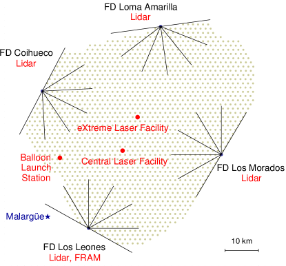
The Pierre Auger Observatory, located about 1 400 meters above sea level near the town of Malargüe, Argentina, is designed to observe extensive air showers created by cosmic rays with energies above eV. Multiple complementary air shower detectors are operated at the Observatory to overcome the shortcomings of any single measurement technique.
The primary instrument of the Pierre Auger Observatory is a large-area Surface Detector (SD) [1, 2], which is used to sample the secondary particles from air showers that reach the ground. The SD is an array of about 1 600 water Cherenkov stations arranged km apart on a triangular grid. The array is deployed over an area of 3 000 km2, and it has a duty cycle of nearly 100%. Thus, data from the SD provide a high-statistics sample of air showers used to study the energy spectrum and arrival direction distribution of the cosmic rays above eV.
While the SD is sensitive to the lateral distribution of secondary air shower particles at ground level, the longitudinal development of showers in the atmosphere is measured using a Fluorescence Detector (FD) of 27 optical telescopes [3]. The telescopes, optimized for the near-ultraviolet band, are located at four sites on the periphery of the SD array: Los Leones, Los Morados, Loma Amarilla, and Coihueco (see Fig. 1). Each site is instrumented with six telescopes deployed inside a climate-controlled building. Together the six telescopes have a field of view covering 180∘ in azimuth and about 0∘ to 30∘ in elevation. At Coihueco, three additional High-Elevation Auger Telescopes (HEAT) have been deployed to observe elevation angles between 30∘ and 60∘ [4].
The fluorescence telescopes are capable of recording the ultraviolet fluorescence and Cherenkov light produced during air shower development. The flux of fluorescence photons from a given point in an air shower track is proportional to d/d, the energy loss per unit slant depth of traversed atmosphere [5]. The Cherenkov emission is proportional to the number of charged particles in the shower above the Cherenkov production threshold, and depends on the energy loss and energy distribution of secondary electrons and positrons in the shower. By observing the UV emission from an air shower, it is possible to observe the energy loss as a function of and make a calorimetric estimate of the energy of the primary particle, after correcting for “missing energy” not contained in the electromagnetic component of the shower [6]. The slant depth at which the energy deposition rate d/d reaches its maximum value is called . By observing for a large set of air showers, the FD data can be used to discuss the composition and the interaction properties of cosmic rays as a function of primary energy [7].
Simultaneous measurements of air showers with the FD and SD are called hybrid events. By performing a joint reconstruction which uses geometrical and timing information from both detectors, it is possible to significantly improve the angular and energy resolution of reconstructed hybrid events with respect to showers observed by the FD alone [8]. Therefore, when FD data are used to produce physics results, only hybrid events are included in the analysis. Moreover, events observed with high quality in hybrid mode are crucial for the calibration of measurements performed using the SD. While the energy of a primary cosmic ray can be estimated using data from the SD alone, the absolute scale of the energy estimator depends on hadronic interaction models of air shower development. To remove this model dependence, the energy scale of the SD is calibrated using a subsample of the hybrid events in which a calorimetric energy measurement from the FD can be compared to an independent energy estimate from the SD [9].
The FD is only operated during nights when UV light from air showers is not overwhelmed by moonlight. Safe telescope operations also require adequate weather conditions (i. e., no rain and moderate wind) and high atmospheric transmittance to assure high data quality. These restrictions limit the duty cycle of the FD to about [10]. As a result, at trigger level the number of events observed with the FD is an order of magnitude smaller than that observed with the SD.
The light profiles recorded with the fluorescence telescopes must be corrected for UV attenuation along light paths of up to km. To estimate the attenuation of light by molecules, aerosols, and clouds, regular atmospheric measurements are performed at the Observatory using UV laser shots, radiosonde launches, optical observations, and cloud measurements in the mid-infrared [11]. The radiosondes provide measurements of the main atmospheric state variables such as temperature, pressure, and humidity, which affect mainly the production of fluorescence light induced by air showers [5, 12], but also the light scattering by molecules. The laser shots and optical observations are used to estimate the aerosol optical depth and the cloud cover over the FD buildings.
The regular atmospheric monitoring performed at the Observatory provides atmospheric data of local conditions with a time resolution of several minutes to several days, depending on the type of measurement. This is sufficient for the bulk of measured air showers. Hourly and daily atmospheric corrections are available for reconstructing individual showers, and the average energy dependence of the atmospheric corrections for the full sample of observed cosmic rays is well-understood [11]. However, because of the massive volume of atmosphere used to perform fluorescence observations – nearly 30 000 km3 – the time and spatial resolution of the atmospheric database is necessarily limited.
For some analyses, it is desirable to provide atmospheric data beyond the regular measurements. For example, the high-energy tail of the data sample used in the SD energy calibration is an important lever arm in the SD-FD fit. Since atmospheric corrections are of utmost importance for the highest-energy showers recorded with the FD, it is sensible to perform dedicated atmospheric measurements at the time and location of high-energy cosmic ray events. Other showers of interest are anomalous longitudinal profiles observed in the FD data. The rate of these showers is expected to be largest at low energies and for light primary masses [13]. Such showers are removed by standard analysis cuts because lumpy profiles are typically caused by atmospheric non-uniformities such as cloud banks or aerosol layers. However, these profiles may also be indicators of exotic primary particles or unusual air shower development. In any analysis which uses longitudinal profiles to search for such exotic phenomena, dedicated monitoring of air-shower tracks is needed to remove events which could be distorted by atmospheric effects.
To provide high-resolution atmospheric data for interesting air showers, we have implemented an automatic online monitoring system which can be used to trigger dedicated atmospheric measurements a few minutes after the air showers are detected. This rapid monitoring trigger was commissioned in early 2009 and has been integrated into the regular monitoring schedules of several of the atmospheric monitoring subsystems. In this paper, we will discuss the operation and performance of the rapid monitoring program. In Section 2, we describe the Pierre Auger Observatory and review the standard atmospheric monitoring program. The implementation of the online atmospheric monitor is discussed in Section 3. The integration of rapid monitoring into the radiosonde, lidar, and optical telescope subsystems is discussed in Sections 4, 5, and 6, along with a selection of interesting showers. We conclude in Section 7.
2 Atmospheric Monitoring
As described in Section 1, measurements of air showers with the fluorescence telescopes are affected by fluctuations in atmospheric conditions, and so extensive atmospheric monitoring is carried out at the Observatory [11]. The locations of the SD, FD, and the atmospheric monitors described in this work are shown in Fig. 1.
Atmospheric measurements are stored in several multi-gigabyte databases for use in the offline reconstruction of air showers. The time resolution of the measurements ranges between five minutes (in the case of cloud data) to one hour (in the case of aerosol data) to several days (in the case of altitude-dependent atmospheric state variables). The spatial resolution is limited, the altitude-dependent atmospheric state variables are assumed to be horizontally uniform across the SD array, while aerosol conditions and state variables from ground-based weather stations are treated as uniform in the region around each FD building or station, respectively. The systematic uncertainties introduced by the limited resolution of the database have been estimated and are reported as part of the uncertainty in the FD energy scale provided for the SD energy calibration [11, 14]. Due to the correlation between the reconstructed energies of air showers and the distances at which they are observed in the telescopes, the uncertainties increase linearly with energy [11].
2.1 Atmospheric State Variables and Site Models
Air temperature, pressure, wind speed, and humidity are recorded at ground level by weather stations at each FD building and at the Central Laser Facility (see Fig. 1), and between 2002 and 2010 a weather balloon program was operated at the Pierre Auger Observatory. Prior to mid-2005, the radio soundings were performed in ten dedicated campaigns, each lasting two to three weeks, with an average of 10 launches per campaign. Between mid-2005 and end of 2008, the balloon launches were performed more regularly – about every five days and independently of FD data-taking.
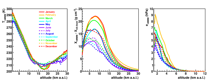
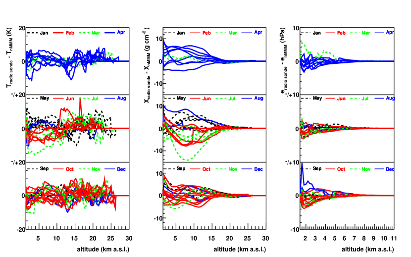
To compensate for the missing information between the radiosonde measurements, average models of monthly conditions were constructed. The first version of these Malargüe Monthly Models (MMM) contained vertical profiles of atmospheric temperature , pressure , density , and atmospheric depth derived from pre-2005 weather data from Malargüe and data from Córdoba and Santa Rosa, Argentina, the sites nearest Malargüe with publicly available radio sounding measurements [16]. The local measurements were supplemented with external data because of the low measurement statistics at the Observatory when the models were constructed. By 2009, the number of balloon flights over the Observatory was sufficient to re-evaluate the profiles and construct improved models with an additional average profile of the water vapor pressure [11]. These new Malargüe Monthly Models (nMMM) were derived from 261 local radio soundings performed between August 2002 and December 2008.
The nMMM profiles comprise vertical profiles of , , , , and specified between km and km above sea level in steps of m. Of the 261 radio soundings used to construct the models, 32 were discarded during construction of the vapor pressure profiles due to contamination of the balloon flights by high cloud coverage. Above km, the vapor pressure has been set to zero.
The local radio soundings provide reliable and unbiased measurements of the monthly average profiles between about km and the burst altitude of the balloons. The burst altitude was typically at km, with a few balloons reaching a maximum altitude of km. Data from the five ground-based weather stations at the Observatory were used to extrapolate the profiles down to km222For technical reasons during air shower reconstruction, the profiles need to go beyond the lowest surface height.. Above the altitude of balloon burst, the data have been extrapolated using values from the 2005 monthly models. The nMMM profiles of , , and are shown in Fig. 2, top row.
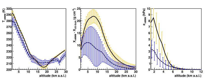
The uncertainties of the model atmospheres are quite large. For temperature, the RMS fluctuations at ground level range between K during austral summer to K during austral winter333Austral summer refers to the months of December, January and February, austral winter corresponds to June, July and August.; at km, the RMS spread is K during austral autumn and K during austral spring. Atmospheric depth varies mainly between km and km. The RMS spread of atmospheric depth at ground ranges between (summer) and (winter); the largest RMS, at km, is about . Above km, the depth uncertainties are below . The vapor pressure RMS at ground is hPa (summer) and hPa (winter), but is well below hPa above km. For illustration, the uncertainties are plotted exemplarily for February (austral summer) and August (austral winter) in Fig. 2, bottom row.
2.2 Optical Transmission and Cloud Detection
During the 15 to 19 nights per lunar cycle that are dark enough to operate the fluorescence telescopes, hourly measurements of the aerosol optical depth [11, 17] are made as a function of altitude with two central laser facilities [18] and four lidar stations [19]. In addition, an optical telescope called the ph(F)otometric Robotic Atmospheric Monitor (FRAM) [20] is used to measure the integral aerosol optical depth inside and outside the field of view of the FD building at Los Leones. Finally, the cloud coverage at the Observatory is measured with the lidar stations and infrared cameras located at each of the four FD sites [11].
There are four lidar stations, one per FD site, and during regular operations the lidars are used to scan the atmosphere outside the field of view of the FD telescopes. Currently, the scans are used to retrieve the mean cloud cover and the lowest cloud height during each hour of FD measurements. IR cloud cameras provide complementary 2D images of the whole field of view every five minutes [11]. A direct combination of these two pieces of information is used to provide a three-dimensional map of clouds above the Observatory, but not without ambiguities. For instance, inspection of the lidar data has shown that multiple cloud layers are present above the site about of the time; a mismatched altitude may be associated to the clouds detected by the IR cameras since different cloud layers cannot be easily distinguished in the IR images.
FRAM is a robotic optical telescope with primary mirror diameter of 0.3 m located about 30 m from the fluorescence detector building at Los Leones. The instrument was installed primarily to determine the wavelength dependence of the extinction caused by Rayleigh and Mie scattering. This goal is achieved using the photometric observations of selected standard (i .e. non-variable) stars, and recently also using the photometric analysis of CCD images. The results of this primary mission are presented in [21]. Since its installation in 2005, the FRAM telescope has also been involved in automatic observations of optical transients of gamma-ray bursts. This program is very successful and several light curves of transients were already observed, including one uniquely bright GRB afterglow [22].
3 The Rapid Atmospheric Monitoring Program
Atmospheric uncertainties grow as a function of primary particle energy because of the energy dependence of the longitudinal development of air showers, which affects the geometry of observable showers within the field of view of the FD [11]. An improvement in the resolution of the atmospheric monitoring data can be achieved by triggering measurements of the atmosphere within a suitable time interval after the detection of high-energy showers above a certain threshold (e. g., eV). Such triggers have been implemented for the individual weather balloon, lidar, and FRAM optical telescope subsystems.
During the FD data taking, an automated process is used to collect event data from the FD and SD, build and reconstruct hybrid events, and send the reconstructed shower parameters to the atmospheric monitoring subsystems participating in the rapid monitoring program. Each subsystem performs individualized cuts on the shower parameters, and if the shower is a candidate for special monitoring – e. g., it has a well-observed track and is of a particularly high energy – an atmospheric measurement is performed either in the vicinity of the shower track (for transmission measurements) or above the Observatory with meteorological weather balloons. In this manner, the time resolution of the atmospheric measurements can be reduced from hours to minutes (for the lidars and the FRAM) or from days to hours (for the weather balloons) with respect to the arrival time of an interesting shower. Moreover, the lidar stations and the FRAM are able to directly probe the atmosphere along the shower-detector plane – the plane defined by the position of the FD telescope and axis of the shower – reducing the uncertainties introduced by the assumption of horizontally uniform atmospheric layers in the weather databases.
The rapid atmospheric monitoring system consists of three components: an online event builder that merges shower data as they are sent to the Observatory campus in Malargüe; a hybrid reconstruction that uses all the detector and calibration data that are available immediately after a shower is detected; and a broadcast program that notifies the atmospheric subsystems of the detection of a hybrid event. The programs are designed to run without human intervention during FD measurements. We discuss the software components in Section 3.1 and review the performance of the reconstruction in Section 3.2.
3.1 Online Event Builder, Reconstruction, and Broadcast
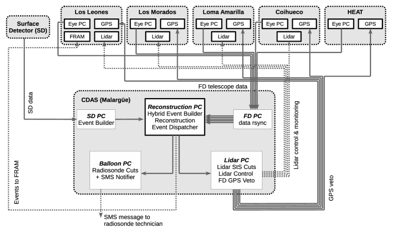
The flow of data between the Observatory campus and the atmospheric subsystems is shown in Fig. 3. During FD measurement periods, data from the fluorescence telescopes are transferred to Malargüe in a 20-second cycle. Simultaneously, triggers and recorded data from the surface array are sent to the SD Central Data Acquisition System (CDAS), a computer cluster and disk array located in Malargüe. Due to a polling delay that allows the SD communications system to collect data from across the array, surface station data typically arrive in the CDAS to minutes after the detection of an air shower.
Once the SD and FD data are available in Malargüe, a fast online event builder produces air shower data in the standard hybrid format. The data are reconstructed using a version of the Auger reconstruction software [23], which is named , modified for online running. The online reconstruction is configured to use the latest available detector and calibration databases, and it is kept in sync with releases of the software. This is to keep the results of the online reconstruction as close as possible to the standard offline444While will refer only to the software framework, “offline” is meant to describe processes that happen several days to months after the measurement. reconstruction. However, since the non-event databases are typically updated on timescales of 4-6 months, some drifts between the online and offline reconstructions are unavoidable.
In the offline reconstruction, large-particle scattering by aerosols is estimated using atmospheric measurements. It is not possible to use real-time atmospheric monitoring data in the online reconstruction, so instead an average parametric model of aerosol scattering in Malargüe is used. Rayleigh scattering by molecules is calculated using the nMMM average monthly models. The systematic uncertainties introduced by the use of average models is discussed in Section 3.2.
Approximately 80 geometry, quality, and energy parameters from each reconstructed shower are written to disk on the Reconstruction PC (cf. Fig. 3). As they are saved to disk, the events are also transferred to the atmospheric monitoring subsystems (Balloon PC, Lidar PC, and FRAM) via network broadcast. Client programs in the atmospheric monitors are used to perform cuts on the hybrid data and issue triggers based on the specialized measurements performed with each instrument (see Sections 4, 5, and 6).
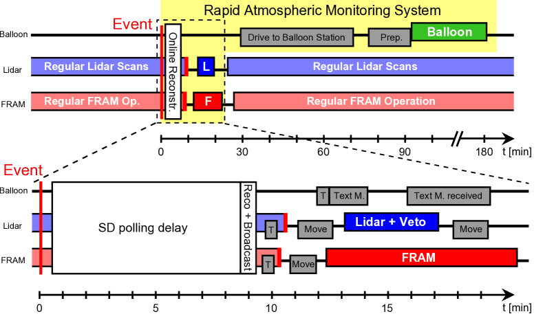
In Fig. 4, a timing diagram is shown for the online reconstruction and the activity within all three subsystems. More details on the individual steps are provided in the corresponding sections. It should be noted that the online reconstruction runs continuously. The pictured timeline shows only the case if an interesting air shower event is identified by subsequent steps. Also, the three systems operate independently, they do not necessarily trigger on the same air shower event because of different trigger criteria.
3.2 Reconstruction Performance
We illustrate the performance of the online reconstruction using hybrid data recorded between March 2009 and March 2011. During this period, 320 hybrid events reconstructed online had energies above eV and passed standard quality cuts based on the event geometry and d/d profile fit [7, 24]. Applying the same cuts to data reconstructed offline produces a set of 382 events during the same period.
Inspection of the events shows that the online and offline sets have only 255 events in common. The discrepancy, and the lower number of online events, is caused by several factors. The number of events reconstructed online is reduced by downtime in the online reconstruction due to various technical problems such as software failures, network crashes, etc. For example, the downtime of the online reconstruction during 2010 was about 15%, which accounts for much of the difference in size between the online and offline event samples. In addition, most of the offline data were corrected for real aerosol conditions, whereas the online reconstruction uses an average model of aerosols above the Observatory. The shower profiles reconstructed online tend to be of worse quality because true aerosol scattering is not taken into account, and so more events fail the offline quality cuts on the shower profile. The migration of events around the quality cuts due to changes in the software versions and databases used in the reconstruction also accounts for an additional reduction in the number of events in common between the online and offline data sets.
It is instructive to compare the common events of the two data sets. In Fig. 5 the differences in the energy and of the common events are plotted. Both distributions contain significant tails, and the energy reconstructed online is systematically higher than the energy reconstructed offline by about 7%. The main cause is the lack of true aerosol corrections in the online data, which accounts for at least half the offset between the two reconstructions [11]. The remainder of the offset is due to differences in software versions between the online and offline reconstructions and the lack of nightly calibration constants in the online reconstruction.
Even though the online reconstruction is affected by a non-negligible downtime, it appears to have performed well since it was first implemented in 2009. The comparison between the online and offline events indicates the presence of a significant systematic bias in the online data because of the use of an average aerosol model. This means that some events which pass the online cuts may not survive the offline analysis cuts. In the absence of real-time aerosol data this is unavoidable. However, it may be possible to tune certain measurements using nearly real-time conditions and hence reduce “false positive” triggers. An example application is discussed in Section 5.2.2.
4 Balloon-the-Shower Program
The use of monthly site models to estimate atmospheric state variables and molecular scattering rather than real-time radiosonde data introduces an uncertainty into the estimated production and transmission of fluorescence light in air showers. This contributes to the statistical uncertainties in the reconstructed energy and position of shower maximum. The total effect is moderate, but it does depend on the shower energy. Between primary energies of eV and eV, the monthly profiles contribute (at eV) and (at eV) to the total energy resolution of about [25], and – to the total resolution of about 20 [7] of the hybrid reconstruction [11, 12, 26]. It is important to note that these numbers are characteristic of a large sample of showers, but the systematic errors in the reconstruction of individual showers can be substantially larger, particularly at high energies. Therefore, it is desirable to minimize as much as possible the atmospheric uncertainties in the reconstruction of high-energy events.
To improve the resolution of the reconstruction for the highest-energy showers, the Balloon-the-Shower program (BtS) was operated between March 2009 and December 2010. Its purpose was to perform an atmospheric sounding within about three hours of the detection of a high-quality high-energy event.
4.1 Performance of BtS
In March 2009, BtS replaced regularly scheduled meteorological radio soundings at the Observatory. The target launch rate was chosen to be three to seven launches per FD measurement period, with each period lasting about 2.5 weeks. The focus of the BtS program was high-energy showers used in the SD energy calibration or the hybrid mass composition analysis; in other words, hybrid events with well-reconstructed longitudinal profiles and energies above eV.
The atmospheric profiles from the BtS program represent an independent data set that can be compared to the nMMM average models. The difference between each BtS profile and its corresponding nMMM profile is plotted in Fig. 6. The width of the deviations is in agreement with the uncertainties of the monthly models described in Section 2.1.
Events passing the online cuts were used to trigger a text message sent to an on-site technician, who then drove to the Balloon Launch Station to launch a weather balloon. Given the lack of automation, the radiosonde flights typically took place only several hours after the detection of a cosmic ray event. To minimize the delay, it was decided to limit the time difference between event detection and balloon launch to a maximum of three hours. This delay was not expected to affect the validity of the radiosonde data, since fluctuations in the vertical atmospheric profiles tend to be much larger between nights than within a single night [27].
4.1.1 Quality Cuts
To trigger a BtS launch, showers from the online reconstruction were required to pass quality cuts used in publications of the SD energy spectrum [24] and the hybrid mass composition [7]. The cuts are listed in Table 1 and were designed to minimize the uncertainty in shower energy and . In fact, the cuts used for BtS are moderately stricter than those used in [7, 24] to account for the systematic uncertainties in the online reconstruction described in Section 3.2.
Cuts (1) and (2) select showers in which the reconstructed energy and the position of shower maximum are reliably estimated. Cut (3) removes showers in which is less than from either the minimum or maximum observed depth of the shower track. This reduces the possibility that is mis-identified and also improves the reconstructed d/d profile. Cut (4) is a standard geometry cut that ensures the surface station with the largest signal (i. e., the one used for timing in the hybrid reconstruction) is close to the shower core. Cuts (5) and (6) are indicators of the quality of a Gaisser-Hillas parametric fit to the longitudinal shower profile [6, 28]. Cut (5) is effective at removing showers obscured by clouds and other atmospheric non-uniformities, since the profiles of such showers deviate strongly from a Gaisser-Hillas curve. This cut also removes possible exotic air shower candidates that are covered by the other two subsystems (cf. Sec. 5.1.3 and Sec. 6.3.2), as they are not the main focus of the BtS program. Cut (6), a difference between a linear fit and a Gaisser-Hillas fit to the longitudinal profile, removes faint, low-energy showers from the trigger sample. The fraction of rejected events of the cuts are included in Table 1.
| Quality Cut | Rejected Events | |
|---|---|---|
| (1) Energy uncertainty | 47.5% | |
| (2) uncertainty | 59.5% | |
| (3) Field of view | well observed | 8.8% |
| (4) Distance to SD with highest signal | 0.5% | |
| (5) Quality of Gaisser-Hillas (GH) fit | 5.3% | |
| (6) Comp. of GH with linear fit | 36.8% | |
| Energy threshold | EeV | 99.3% |
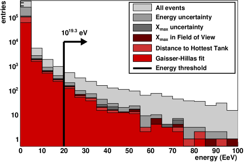
The hybrid events recorded between January 2006 and January 2009 were used as a tuning sample to set the rate of BtS triggers. The effect of the cuts are shown as a function of energy in Fig. 7. To reach the desired number of atmospheric soundings – to per year, or about to per FD measurement period – it was necessary to further reduce the size of the event sample with a cut on the reconstructed shower energy. The energy threshold, determined from the tuning sample, was
| (1) |
4.1.2 Trigger of Weather Balloon Launches
After a shower passed the automatic BtS trigger, a short message containing the date and time of the event was sent to the mobile phone of an on-site technician. If the message was received, the technician would drive to the Balloon Launch Station and proceed with the atmospheric sounding within three hours of the event.
Between March 2009 and December 2010, 100 text messages were sent to the technician. From these 100 triggers, 52 balloons were launched successfully. Some messages were received while a radiosonde was already in flight, due to the tendency of high-quality, high-energy observations to cluster during very clear, cloudless nights. Therefore, 62 BtS triggers were covered by the 52 flights. The remaining triggers, about one-third of the total, were lost due to technical issues such as a hardware failure at the Balloon Launch Station in August 2009 (11 events), problems with the transmission of the text messages, or other failures in the radiosonde flights.
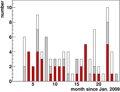
The BtS statistics between March 2009 and December 2010 are shown in Fig. 8. Note that the chart shows events reconstructed using the offline reconstruction (and after quality cuts were applied) and not the online reconstruction. During the period of BtS operations, 88 events reconstructed offline passed the BtS cuts. Of these, 59 were also identified online, meaning that out of the 100 events which triggered a text message, 41 do not survive the BtS cuts after offline reconstruction. Some did not satisfy the BtS cuts, while others fell below eV. Of the 59 common events, 35 were covered by a weather balloon launch. If the energy cut is relaxed slightly to eV, 51 offline events are covered by a balloon launch.
4.2 Air Shower Reconstruction using BtS Data
To evaluate the effectiveness of the BtS program, we have reconstructed hybrid events covered by the radiosonde launches conducted since March 2009. The results are compared to a reconstruction that uses the nMMM average monthly conditions, as well as more real-time conditions given by the Global Data Assimilation System (GDAS) [29]. GDAS is a global atmospheric model based on meteorological data and numerical weather predictions. Altitude-dependent profiles of atmospheric state variables such as , , and are provided on a latitude-longitude grid. The GDAS database contains profiles which are useful for the needs of the Pierre Auger Observatory with a time resolution of three hours starting in June 2005. Hence, the database covers not only the period of BtS launches, but also most of the period of data-taking at the Auger Observatory. GDAS data were made available to the air shower analysis of the Auger Observatory beginning in spring 2011 [30].
4.2.1 Effect of BtS Profiles and Model Atmospheres on the Reconstruction
To study the effect of the BtS data on the reconstruction of air shower profiles, we have reconstructed the 62 hybrid events covered by 52 BtS launches. This data sample contains 52 events which pass all quality cuts consisting of 90 individual fluorescence profiles after accounting for events observed in stereo with multiple telescopes. We also compared the reconstruction using BtS data to those using nMMM and GDAS model profiles. In case of reconstructions using nMMM, two more events where discarded by cut criteria, thus only 50 events are contained in this reconstruction data sample. In all cases, we have accounted not only for the effects of the atmospheric profiles on light scattering, but also for the effects of temperature, pressure, and humidity on fluorescence light production [5, 11, 31]. For the fluorescence light calculation, experimental data from the AIRFLY experiment [32] and conference contributions [33] from the AIRFLY collaboration were used.
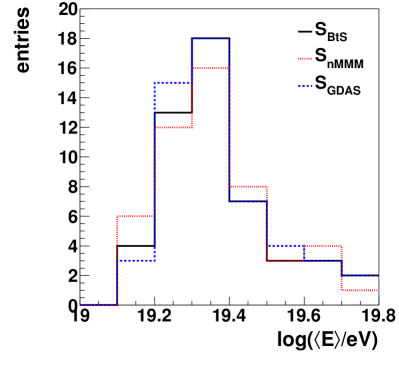
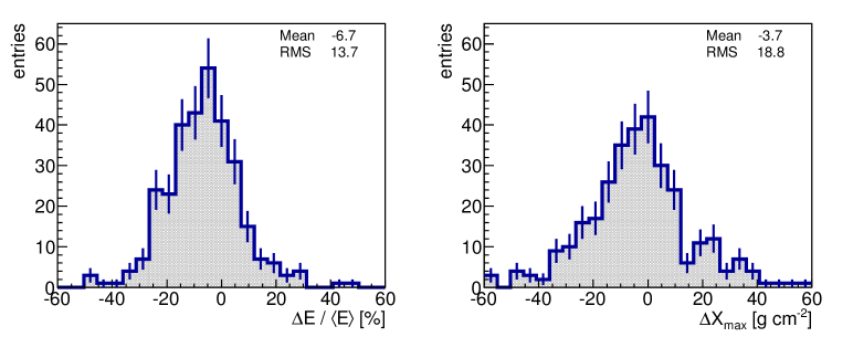
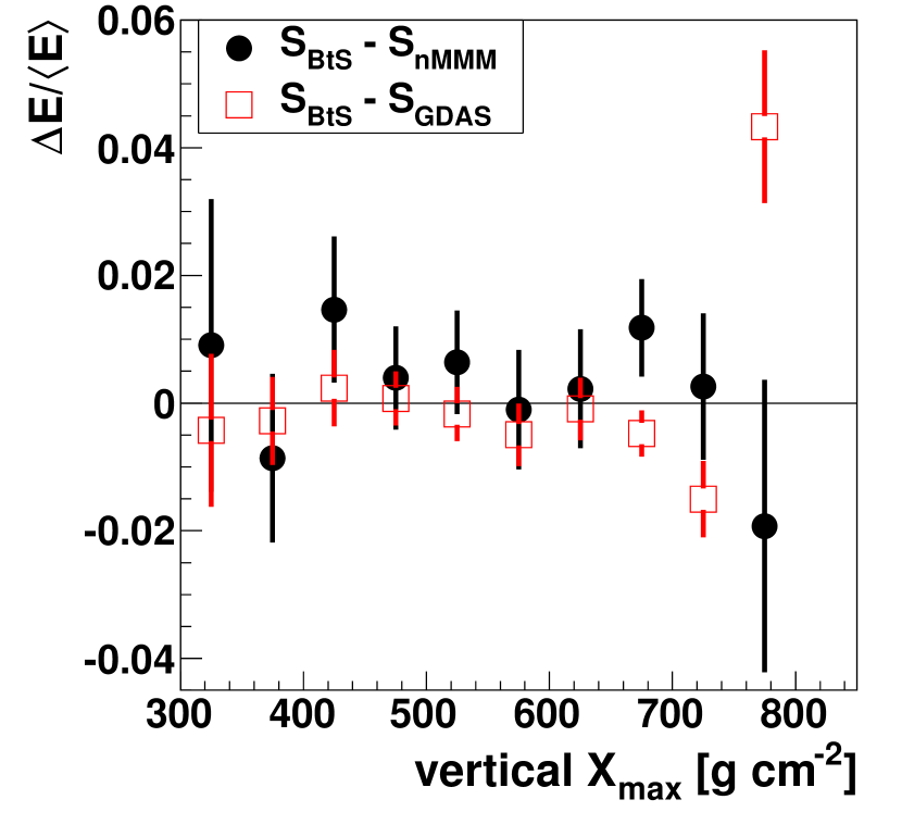
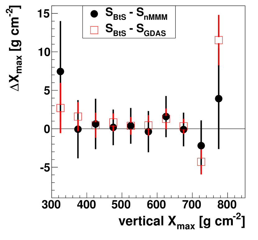
In the study, we devote our main attention to the reconstructed cosmic ray energy and depth of shower maximum of the air shower profiles. The energy distribution of the reconstructed events is provided in Fig. 9. For air showers detected by more than one telescope, the weighted mean of the shower observables is used. All events represented by the solid line are reconstructed using the atmospheric profiles gathered within the BtS program, S. Reconstructions applying the monthly atmospheric conditions as described by nMMM, S, are displayed with a dotted red line. The third set of reconstructed air showers, S, is plotted as a dashed blue line and was obtained using the corresponding model atmospheres from GDAS. The three distributions agree well within the systematic uncertainty of the hybrid energy reconstruction [14]. The overall systematic uncertainty is 22%, whereof 1% are contributions due to atmospheric uncertainties [9] which are discussed here. Note that some events have spilled below the energy threshold of eV because of the systematic energy shift between the online and offline reconstructions. The mean energy of the event sample is eV.
| [%] | RMS() | [ ] | RMS() [ ] | |
|---|---|---|---|---|
| BtS – nMMM | 0.5 | 2.3 | 0.3 | 6.6 |
| BtS – GDAS | 0.2 | 1.2 | 0.5 | 3.3 |
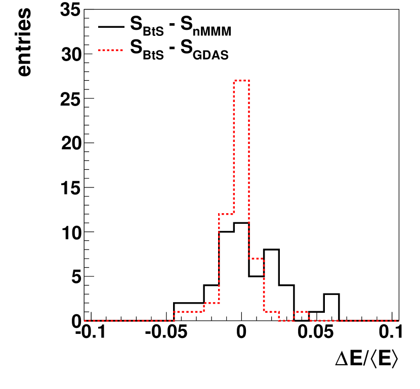
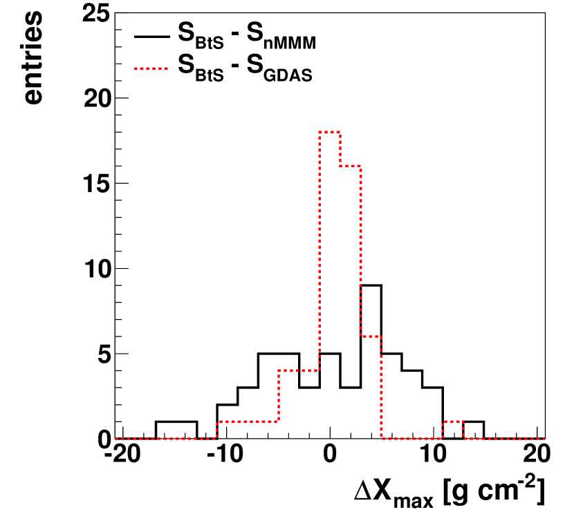
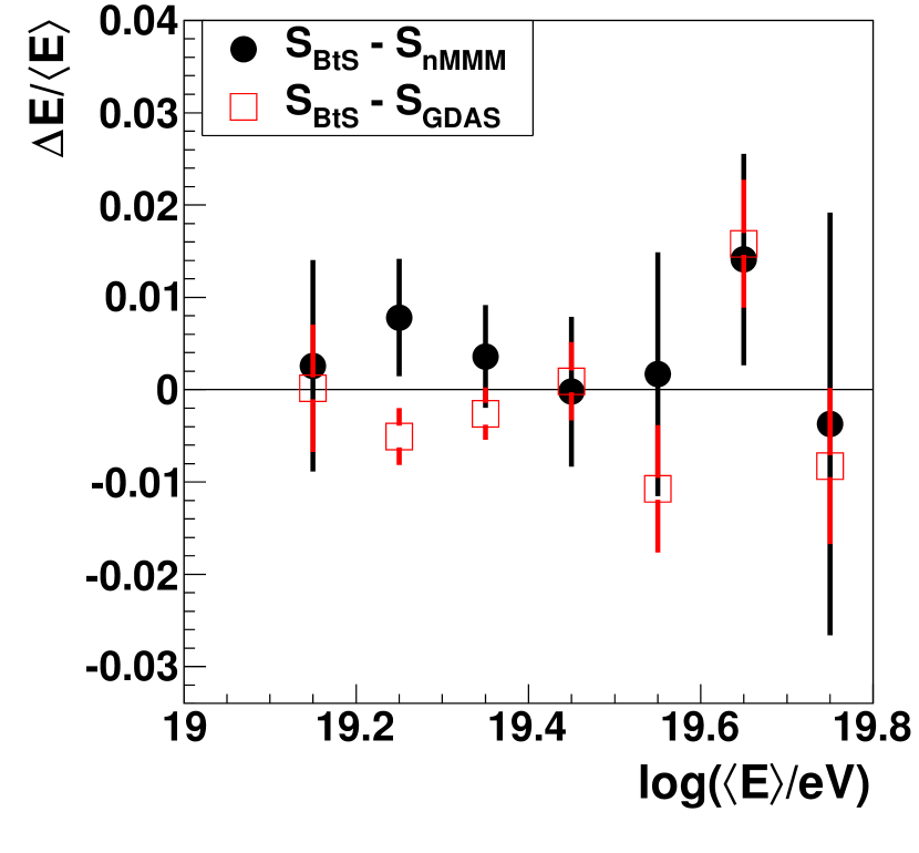
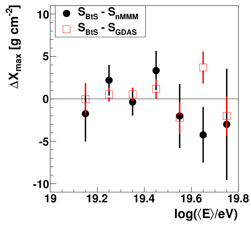
In Fig. 11 and Fig. 11, the distributions of the energy difference and between the S and S events (solid line) and the S and S events (dotted line) are plotted, respectively. The quantity is the average of the energies reconstructed with each pair of atmospheric profiles. The mean differences and widths of the distributions for both and are listed in Table 2. For the BtS-nMMM comparison, the most extreme differences of about and are found for and , respectively. The width of the distribution for the BtS-GDAS comparison is smaller because the time resolution of the GDAS profiles is much finer than that of the monthly models. The comparison indicates that the GDAS data provide a reasonable description of the local conditions on time scales of a few hours.
Finally, it can be concluded that the systematic uncertainties of the energy (22%) and of (13 [7]) are hardly reduced by applying actual atmospheric profiles in the reconstruction of extensive air showers instead of applying adequate local models. The resolution of and can be slightly reduced by 0.3% and 1.1 , respectively.
4.2.2 Study of Systematics
In this section, we describe several possible systematic effects in the event reconstruction:
-
1.
Energy dependence of the and distributions;
-
2.
Seasonal effects;
-
3.
Dependence on vertical .
We investigate systematic effects using the differences in the reconstructed energy and after using the BtS, nMMM, and GDAS data in the reconstruction. The energy dependence of the distributions of and is shown in Fig. 14. The S-S comparisons are plotted with black points, while the S-S comparisons are plotted with red squares. No energy dependence is observed.
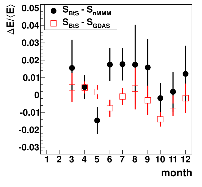
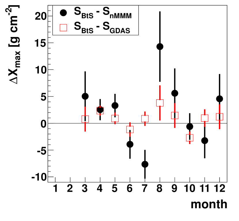
Seasonal effects have been investigated by plotting the energy and differences according to the calendar month (Fig. 14). While the primary energy does not show any signs of seasonal dependence, there are larger fluctuations in in particular during the austral winter when using the nMMM profiles instead of the BtS profiles in the reconstruction.
The third systematic dependence of interest is vertical (see Fig. 14). Vertical is the projection of the inclined shower track to the vertical, which we use to correct for the different inclination angles of the air showers and establish a clear relationship to the layering of the atmosphere. For both and , no dependence is obvious. Note that the entry for vertical between 750 and 800 corresponds to only one event, since only one air shower profile has been detected with such a deep after applying all quality cuts of the BtS program. This particular shower entered the Earth’s atmosphere quite vertically with a reconstructed zenith angle of about 12∘.
Finally, we performed additional searches for any dependence of and on fluorescence detector location, on the distance of the core position from FD telescope, and on some further effects induced by the incoming geometry of the air shower. The dependence of and on these parameters is negligible in all cases.
5 Shoot-the-Shower Program
The purpose of Shoot-the-Shower (StS) is to initiate lidar scans of the shower-detector plane created by the image of an air shower in an FD telescope. The motivation is to identify atmospheric non-uniformities – especially clouds – that obscure light from the shower as it propagates to the FD telescopes. Such non-uniformities may not be present in the hourly atmospheric databases, and so StS is intended to supplement the cloud identification performed using the regular lidar scans.
An hourly cloud coverage below is required for hybrid events to be used in the analysis of the mass composition and energy spectrum of the cosmic rays observed at the Pierre Auger Observatory [7, 24]. This cut may still allow sparse clouds to affect the FD measurements, so one of the main goals of StS is to observe showers which pass the cloud coverage cuts but fail the longitudinal profile cuts. StS can be used to verify that the profile quality cuts are removing showers contaminated by weather effects and not also removing physically interesting showers from the event sample. The StS trigger has also been adjusted to support the search for anomalous longitudinal profiles due to hadronic interactions [13]. These two running modes are described in the following sections.
5.1 Performance of StS
Each lidar station contains a steerable telescope and a µJ Nd:YLF laser with a central wavelength of nm. The telescope collects backscattered laser light, and the analysis of the return signal can be used to infer the presence of aerosols and clouds along the light path [19]. Because the laser wavelength is in the center of the UV acceptance window of the FD telescopes [3], the operation of the lidar must be carefully controlled to avoid triggering the FD telescopes with scattered laser light. The implementation of the control system for StS is briefly described in Section 5.1.1. In Sections 5.1.2 and 5.1.3, we describe the general-purpose and anomalous-profile StS triggers, respectively.
5.1.1 Full-Site Veto for StS
During normal operations, the lidar stations are programmed to observe the atmosphere above each FD building outside the field of view with an automatic scanning mode called AutoScan. When an StS trigger is received, the lidar stations must stop AutoScan and sweep through the shower-detector plane. This requires the lidars to scan inside the field of view of the FD, creating the possibility of spurious “self-triggers”, or backscattered laser light triggering a nearby FD telescope, and “cross-fires”, or forward-scattered laser light triggering a telescope on the other side of the SD array. To avoid spurious triggers, we have designed the StS mode to inhibit the FD DAQ for the duration of the StS measurement.
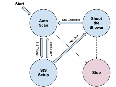
The implementation of the DAQ veto is shown schematically in the state diagram in Fig. 15. Online hybrid events are broadcast to the lidar run control PC running AutoScan in the Malargüe campus (cf. Fig. 3). The run control program analyzes the events for StS trigger conditions. When an event passes the triggers, the run control program calculates a scanning pattern for all four lidar stations and transmits shooting coordinates to the lidar control PCs at the lidar site. When the shooting coordinates are received and automatically confirmed, the run control program sets a DAQ VETO bit in the GPS servers at each of the FD buildings. After the veto is set and confirmed by the run control software, the AutoScan is paused and the lidar stations begin the StS sweep.
To prevent the lidar run control from deadlocking the FD DAQ, the GPS server VETO bit is set to revert automatically after four minutes, re-enabling FD data acquisition. The lidar StS coordinates are calculated such that the lidar telescopes can safely complete the scan during the four-minute shooting window. If the lidar run control program in Malargüe loses network communication with the lidar stations at any time during AutoScan or StS, the stations will revert to a partial shutdown mode to prevent uncontrolled laser interference with the FD telescopes.
5.1.2 General-Purpose StS Trigger
The first set of quality cuts applied to StS candidate events, given in Table 3, are designed to include the showers that are likely to become part of the main high-energy hybrid data set. However, the cuts are also loose enough to accept events with unusual “dips” and “spikes” in the longitudinal profile. Such features are typically caused by strong attenuation and multiple scattering by clouds and aerosol layers. Including these events in the StS sample can allow us to investigate why some longitudinal profiles do not pass strict profile cuts. We also considered the possibility that such events might be recovered for use in the analysis in the future, if the cloud-affected portions of the longitudinal profiles could be removed.
| Quality Cut | Rejected Events | |
|---|---|---|
| (1) Field of view | 45% | |
| (2) Gaisser-Hillas (GH) fit | , and , | 30% |
| , and | ||
| (3) Energy uncertainty | , and , | 99.7% |
| , and | ||
| (4) Track length | 4% | |
| (5) Local zenith angle | 33% | |
| (6) FD-core distance | 1% |
Cuts (1), (2), and (4) in Table 3 ensure a reliable reconstruction of the shower energy and the depth of shower maximum. However, cut (2) on the shower profile is loose enough to accept events which are not well-described by a Gaisser-Hillas function. This includes bumpy events, or profiles with a strong asymmetry. The purpose of cut (3) on shower energy is to heavily limit the number of lidar scans: from about two per 17 day FD measurement period during austral summer up to two per night during winter. The cut on the zenith angle (5) rejects overly inclined showers, which are problematic because the scan path may be so long that a lidar would not finish the StS within the maximum veto time window of four minutes. Finally, cut (6) excludes air showers which occur at close distances to the FD telescopes, because these do not need corrections for atmospheric transmission. The effects of the cuts are shown as a function of energy in Fig. 16.
Events which are analyzed by the lidar run control program are also removed if the corresponding shower has occurred more than minutes in the past. This is to ensure that the StS measurements accurately describe the distribution of clouds and aerosols when the shower was observed. During times when both the online reconstruction and the lidar system were operational, no events had to be rejected because of this criterion.
5.1.3 Anomalous Profile (“Double-Bump”) StS Trigger
In March 2011, a second StS trigger was implemented to aid in the search for anomalous longitudinal profiles. This search is motivated by recent simulations which indicate that in a small fraction of air showers, leading particles can penetrate deeply into the atmosphere before interacting and creating another maximum in the shower profile [13]. The longitudinal profile of such showers will have two peaks – hence “double-bump” showers – which can be fit using a sum of two Gaisser-Hillas functions. The fit yields two values of ( and ) for the two peaks in the profile.
| Quality Cut | Rejected Events | |
|---|---|---|
| (1) Double GH fit successful | — | |
| (2) Field of view cut | ||
| (3) Double GH improvement |
The goal of StS in this analysis is to help discriminate double-peaked fluorescence profiles caused by hadronic interactions from the much larger background of double-bump showers caused by scattering due to aerosols and clouds. Based on hybrid events observed between January 2004 and December 2010, a set of simple cuts has been developed to select double-bump events for StS. The cuts are listed in Table 4, and simply require that: (1) a sum of two Gaisser-Hillas functions can be fit to the longitudinal profile; (2) both and are within the FD telescope field of view; and (3) fitting the profile with two Gaisser-Hillas functions results in a substantial improvement over a single Gaisser-Hillas fit.
We note that the double-bump trigger is not energy-dependent; in principle low and high-energy showers can give rise to double-peaked profiles. Therefore, to prevent the energy cuts described in Section 5.1.2 from eliminating double-peaked events, the double-bump trigger has been set to supersede the standard StS trigger. In addition, we note that the cuts in Table 4 were tuned on a data set in which nights with heavy cloud and aerosol contamination were removed using the atmospheric databases. Therefore, the trigger is effective insofar as clouds and aerosols can be removed in real time. This issue will be discussed further in Section 5.2.
5.2 Results
Between January 2009 and October 2011, 112 air showers triggered an StS scan and were successfully reconstructed offline. Of these showers, 58 triggered telescopes at one FD site; 40 were observed in stereo mode at two FD sites; eight were observed at three FD sites; and six events were observed at all four FD sites. In total this sample comprises 186 individual fluorescence profiles. The reconstructed ground impact (or core) locations of the 112 air showers are shown in Fig. 18, superimposed on the SD array. The energies of the events, reconstructed offline with all available calibration and atmospheric databases, are shown in Fig. 18.
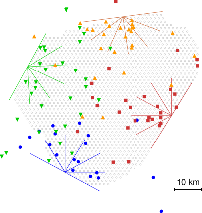
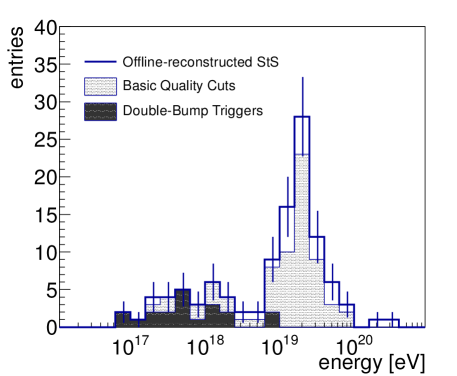
Among the notable features in Figs. 18 and 18 are showers with core locations not contained inside the boundaries of the array, as well as several very high-energy events ( eV). These features are due to events in which the SD “signals” corresponding to the FD longitudinal profiles were identified by the software as coincident noise. Therefore, the showers were reconstructed in FD-monocular mode using no SD data, rather than hybrid mode. Such events are easily removed from the data by applying cut (4) listed in Table 1. Applying this cut removes the showers with cores not contained in the SD array, as well as the high-energy events in Fig. 18. The cut was intentionally omitted from the StS trigger because FD-only events are still useful for systematic studies if they are observed in stereo mode (cf. [34]).
5.2.1 Air Shower Analysis using StS data
Our main interest in this study is the effect of StS on the standard hybrid analyses, and so we cut all events not reconstructed in hybrid mode. This reduces the sample to 89 events (146 FD profiles). We also require that the remaining FD profiles have a corresponding StS scan from the lidar station located at the same FD site. E.g., an air shower observed at Los Leones must have an StS scan from the lidar at Los Leones. This requirement reduces the event sample to a final size of 62 events (86 FD profiles). The reduced statistics are caused by down time of individual lidar stations during repair and maintenance periods.
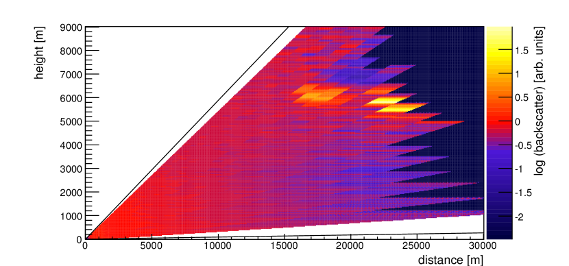
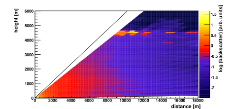
The StS scans have been analyzed in order to find incidental clouds along the shower path. An automatic cloud detection algorithm used to estimate cloud coverage at each FD site [35] has been adapted for these scans by implementing a progressive re-binning of the signal trace. This allows for an extension of the lidar range up to 30–35 km, depending on atmospheric conditions. An example StS scan is shown in Fig. 19.
Of the 62 StS scans, clouds have been detected in 27. Since the quality cuts used in most hybrid analyses require periods with less than cloud coverage, the StS is particularly important if it identifies clouds during otherwise clear periods. It appears that such cases are rather uncommon; of the 27 StS scans affected by clouds, only two occurred during periods of low cloud coverage. In both cases, the clouds observed were at rather high altitudes (7 km and 10 km, respectively) and did not appear to affect the transmission of light between the shower axis and the observing telescopes.
5.2.2 Analysis of Double-Bump Triggers
The StS double-bump trigger began operating during the FD measurement period of February-March 2011. This was a period marked by significant broken cloud cover nearly every night of the data taking. As discussed in Section 5.1.3 and Table 4, the double-bump cuts were tuned on a cloud-free data set, making the double-bump trigger susceptible to false positives in the real data where clouds were not removed. In fact twenty double-bump triggers were recorded and shot during this measurement period, an average of 1.3 per night. Inspection of the data confirmed that all of the showers were affected by atmospheric scattering.
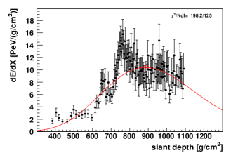
A representative double-bump event, observed at Loma Amarilla, is shown in Figure 20. The fluorescence light longitudinal profile (Fig. 20) exhibits spikes at slant depths of and . For this shower geometry, the spikes correspond to altitudes of about 3.6 km and 4.7 km above the FD site Loma Amarilla, which is at an altitude of about 1.48 km above sea level. Such spikes are characteristic of multiple-scattering of light as the air shower enters a cloud layer. Inspection of the StS profile recorded by the Loma Amarilla lidar station confirms the presence of a reflective cloud layer in the shower-detector plane at the expected altitude that is responsible for the spikes.
Unfortunately, an analysis of the first double-bump profiles reveals that all of the triggers were clearly spurious events created by obscuring clouds. In order to avoid wasting valuable time shooting low-energy showers affected by clouds, it is clear that some kind of real-time identification of coverage will be necessary. This may already be possible with existing lidar data. The cloud-detection algorithm used on the AutoScan data and described in [35] is both fast and robust, and could be applied online. An online cloud coverage estimate could then be used to suppress StS after double-bump triggers whenever the coverage was over some minimum threshold, such as . The real-time identification of cloud coverage and its application to StS is currently under study.
6 Rapid Monitoring with FRAM
The (F/Ph)otometric Robotic Atmospheric Monitor, or FRAM telescope, is capable of carrying out rapid monitoring observations. FRAM is operated as a passive scanner – i. e., observations do not require the use of lasers or light flashers – and so it does not introduce any dead time into the FD data acquisition. Therefore, unlike the lidars, there are no limitations on the use of FRAM in the rapid monitoring program. FRAM can be programmed to scan the shower-detector plane of interesting showers and record CCD images along the plane. Since the FRAM telescope is located close to the FD building at Los Leones, its use in the rapid monitoring program is limited only to hybrid air showers observed from Los Leones. From this location, sequences of CCD images are produced along the shower-detector planes of observed cosmic ray events.
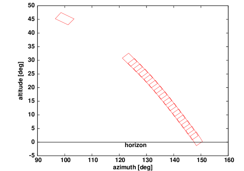
The FRAM telescope is equipped with two CCD cameras. A wide-field555Finger Lake Instrumentation (FLI) MaxCam CM8 with Carl Zeiss Sonnar 200 mm telephoto lens. (WF) camera is used to measure the atmospheric extinction along the shower-detector plane, and a narrow-field666Since June 2010, we have used the Moravian Instruments CCD camera G2. Before June 2010, we used another FLI MaxCam CM8. Both cameras have been situated at the focus of the main 30 cm-diameter telescope. (NF) camera is used to calibrate the WF images. The field of view of the WF camera is () in azimuth (aligned with right ascension) and () in elevation (aligned with declination). Hence, a shower traversing the whole field of view of an FD telescope is typically covered by 10 to 20 CCD images (Fig. 21). The first image of the sequence is oriented along the axis of the cosmic ray air shower to search for optical transients that could be associated with event, assuming the primary cosmic ray was a neutral particle. The field of view of the NF camera is about () in right ascension and () in declination, and is centered within the WF camera image.
The images recorded with FRAM are analyzed automatically. First, stars in the image are identified and their observed magnitudes are compared with values from a catalog, allowing computation of the measured atmospheric extinction along the line of sight to each star. As there are typically several hundred identifiable stars in each image, it is possible to monitor the extinction along the shower track with high angular resolution. Variations of the resulting extinction coefficient reveal the presence of clouds or prominent aerosol layers.
Currently, the rapid monitoring observations of FRAM are carried out using the Johnson-Cousins B filter (central wavelength 435 nm; FWHM 100 nm) of the UBVRI set of astronomical filters [36]. Both cameras are equipped with the same set of filters. For the comparison with FD observations, the Johnson-Cousins U filter (central wavelength 360 nm; FWHM 64 nm) would be more suitable, but the transmission of the WF camera of the FRAM telescope decreases very quickly below 400 nm, and in the U filter we typically detect only several stars, too few for a successful computation of the extinction along the shower-detector plane.
Following astronomical convention, the light extinction is obtained by calculating the difference between the measured magnitude of observed stars and the tabulated magnitude available in star catalogs [37]. This difference depends on the optical path length through the atmosphere, known in astronomy as the airmass . The airmass is a zenith-dependent quantity similar to slant depth that is expressed with respect to the total atmospheric overburden observed along a vertical path between sea level and the top of the atmosphere. From these quantities, the extinction can be expressed as an extinction coefficient . The extinction coefficient can then be transformed to optical depth using the expression777Since the magnitude system is one of relative brightness, a star that has a magnitude five times greater than that of another star will have a light intensity 100 times greater.
| (2) |
The relatively straightforward analysis of the CCD images is an advantage of the FRAM rapid monitoring program, because the analysis can be almost completely automated. Currently, the analysis is carried out offline by the telescope operator, but a fully automated analysis of the FRAM rapid monitoring data is foreseen in the near future.
6.1 FRAM cuts for rapid monitoring
The passive nature of the FRAM observations allows for few constraints in the selection of suitable events relative to the cuts applied for StS (see Sec. 5.1). Currently, three sets of cuts are applied to focus on different types of analyses. The cut parameters can be modified interactively using the RTS2 control software of the telescope [38], even on very short time scales such as one night.
The three sets of cuts are shown in Table 5. Set 1 has been chosen to match the standard selection of high-quality hybrid events used in the analysis of the energy spectrum [24]. Set 2 applies the selection criteria used to identify very deeply-penetrating photon-induced showers, closely matching the cuts used to estimate the photon upper limit with hybrid events [39]. Finally, the third set of cuts is a relaxed version of the standard quality selection. It is designed to exploit the full capability of the FRAM passive monitor, i. e., to perform rapid follow-up monitoring of a very large set of events without interrupting the FD DAQ. The only criterion that is more restrictive in set 3 than in set 1 is the number of triggered PMTs of the FD camera. Without this, set 3 would generate too many triggers. The higher number of PMTs ensures that showers are selected with long tracks that might be better covered by the series of CCD images. The three types of triggers are combined in a logical OR so that a shower fulfilling any one set will trigger rapid monitoring with FRAM.
| Criteria | Set of Cuts | |||
| 1 | 2 | 3 | ||
| (standard) | (photon showers) | (relaxed standard) | ||
| 1. | Reconstructed | eV | eV | eV |
| 2. | Relative uncertainty | — | ||
| 3. | Uncertainty of | — | ||
| 4. | Triggered PMTs | — | ||
| 5. | Profile quality: | 2.5 | 6 | 10 |
| 6. | Comparison of GH and linear fit: | |||
| — | ||||
| — | — | |||
| 7. | Zenith angle of air shower | — | — | |
| 8. | FD telescope-shower viewing angle | — | — | |
| 9. | Hottest station-core distance | m | m | m |
| 10. | Time elapsed since shower arrival | 600 s | — | — |
In March 2011, the FRAM trigger was updated to include a search for anomalous “double-bump” showers. As with lidar StS, the double-bump trigger includes an additional cut on the improvement in the fit of the shower profile when using two Gaisser-Hillas functions. To accommodate such observations, we lowered the energy threshold for the FRAM rapid monitoring triggers to eV in March 2011. However, a dedicated trigger filter for anomalous events is currently being implemented. We describe the search for anomalous shower profiles in Section 6.3.
6.2 Performance of the FRAM telescope
The FRAM rapid monitoring program has operated since November 2009. For the first two months, it was running in a test mode. The cuts given in Table 5 have been applied since January 2010.
To successfully analyze a CCD image, it is necessary to obtain its astrometry. This means identifying the stars recorded in the image using a catalog in order to obtain their exact positions and catalog magnitudes. The shower track is scanned by both CCD cameras at the telescope, but only the wide-field WF camera fully covers the shower track without gaps. Therefore, the data from the narrow-field NF camera are only used to cross-check values from the WF camera. For analysis of the shower-detector plane, we require at least 5 images from the WF camera with astrometry.
Between January 2010 and the end of July 2011, the FRAM telescope received 1 038 triggers for rapid monitoring fulfilling at least one of the three set of cuts described in Table 5. Of those, 586 were successfully observed – i. e., at least 5 WF camera images with astrometry were obtained – with 242 of showers observed in 2010 and 344 in 2011888The observations of showers in periods of bad weather with many clouds do not have a sufficient number of images with astrometry. The rate of successful observations was lower in 2010 due to telescope software and hardware issues, and it has increased in 2011.. The much higher event rate in 2011 was achieved after an upgrade of the telescope control software in March 2011. To allow for more frequent observations, the energy threshold for the triggers in Table 5 was lowered to eV.
The overwhelming majority of the showers, 574 out of 586, passed the relaxed trigger condition (set 3). The standard trigger (set 1) was more restrictive, passing 319 events, as was the photon trigger (set 2), which passed 305 events. The statistics of each trigger filter and the overlap between them are shown in Fig. 22. The overlap between the filters is relatively large; 236 showers passed all three trigger conditions. Only 11 events were exclusively passed by the standard cuts, and just one event was passed by the photon cut alone. However, the photon trigger was affected by a bug before July 2011 that caused events to be lost, so we note that the passing statistics from set 2 are artificially low with respect to the other two filters.
6.3 Results
The output of the FRAM rapid monitoring analysis is a set of extinction coefficients computed in the Johnson-Cousins B filter for each star detected in the WF camera image. A complete shower track is covered by 10–20 WF CCD images (Fig. 23), and so we obtain several hundred to several thousand stars with computed extinction coefficients per track (Fig. 24).
To find obscurations along the line of sight to the shower, we compare the extinction data to a “reference” profile of the extinction in a clear sky. The clear-sky profile is estimated by assuming a uniform atmosphere in which the extinction depends only on the airmass. This gives a zenith-dependent reference curve which can be compared to the extinction coefficients determined using the WF images. For example, the extinction coefficients in Fig. 24 show a dramatic deviation from the clear-sky reference between and elevation due to the presence of the clouds visible in Fig. 23.
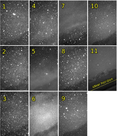
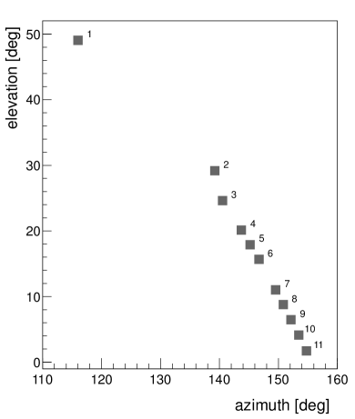
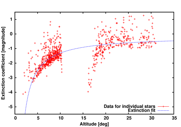
6.3.1 Air Shower Analysis using FRAM rapid monitoring data
To determine whether or not the FRAM observations can be used to identify prominent changes in the extinction which affect the air shower reconstruction, we have searched the 242 events monitored with FRAM in 2010. Within this sample, 13 extinction profiles indicated the presence of clouds.
After inspection of the corresponding longitudinal profiles recorded with the FD telescopes, we have found that 7 of the 13 events also passed the standard quality filter, which includes a tight cut on the profile reconstruction () that tends to remove events affected by clouds. Hence, out of 242 showers which satisfy all standard criteria for high-quality hybrid observations, 7 events (3%) were clearly recorded with clouds in the shower-detector plane.
We note at this point that there are further cuts applied on data for physics analyses, e.g., mass composition studies or building an energy spectrum, which remove events affected by clouds. The most important requires the cloud coverage in the sky above each telescope to be below 20% during a given measurement hour. The cloud coverage is estimated from the lidar AutoScan, in which the lidar stations continuously sweep the high-zenith regions above the FD telescopes. Using the 20% cloud coverage cut, we find that 10 of the 13 cloud-affected FRAM observations will be removed from physics analyses. Of the remaining three events, two were observed during periods of broken cloud coverage with non-zero coverage in the neighboring measurement hours. However, one event was observed during a night in which the lidar data indicates cloud-free conditions during the whole night. After applying the cut on the profile reconstruction quality, only one of these three events passed the standard criterion.
It may appear surprising that the lidar analysis could miss a prominent cloud layer clearly observed with the FRAM telescope, but we must note one critical limitation of the FRAM analysis. Because the extinction is determined using stellar magnitudes, the FRAM measurement only describes the overall atmospheric influence along the line of sight between the FD telescopes and the top of the atmosphere. Using the FRAM alone, it is not possible to determine whether or not a shower profile was observed behind a cloud or in the foreground. In order to determine whether or not a cloud seen by FRAM actually affected a fluorescence profile, it is necessary to look into the FD data themselves to see if the profiles are affected by spurious gaps (absorption) or spikes (multiple scattering). Of the 13 cloud-affected events discussed above, inspection of the data suggests that 11 showers originated behind or partially inside the observed clouds.
This study illustrates the trade-off between passive and active atmospheric monitoring for the FD calibration; the FRAM can operate during FD DAQ without constraints, but the resulting measurements do not have the very useful slant depth resolution of the lidar data.
Nevertheless, the rapid monitoring observations performed with FRAM confirm that the standard selection of hybrid events for physics analysis at the Pierre Auger Observatory is efficiently removing profiles affected by atmospheric scattering. The contamination of the high-quality standard data set by the presence of clouds was found to be of order 1%. The problematic cases within this subsample will be further studied in order to improve future data processing.
6.3.2 Analysis of the double-bump events observed by the FRAM telescope
Because of the short operation of the double-bump rapid monitoring observations, only a few candidates were analyzed for this purpose, and all of them are compatible with profiles containing clouds. As with StS, the anomalous profile trigger will need to be tuned using cloudy and clear data before it can become truly effective.
7 Conclusion
A rapid atmospheric monitoring program has been implemented and operated successfully at the Pierre Auger Observatory since early 2009. The online reconstruction has produced reliable data which have been used to trigger dedicated observations of the atmosphere. Among the showers of particular interest are those initiated by very high-energy cosmic rays, or those with unusual longitudinal profiles. Since the start of rapid monitoring, there have been dedicated balloon flights (until the termination of the balloon program end of December 2010), lidar scans (through October 2011), and observations with an optical telescope (through July 2011). The program has demonstrated that it is possible to perform targeted atmospheric monitoring based on real-time cosmic ray measurements.
The Balloon-the-Shower program was a useful tool for studying short-term variations in the altitude-dependent profiles of the main atmospheric state variables. Using actual atmospheric profiles instead of monthly models in dedicated air shower analyses improves the accuracy of the reconstruction. Unfortunately, this part of the rapid monitoring program imposed a large burden on the collaboration, and due to technical problems the observations fell short of the expected rate. For these reasons, the program was discontinued at the end of 2010. However, the measurements have had a positive effect, as we have used BtS measurements to confirm the validity of atmospheric profiles from the Global Data Assimilation System (GDAS). Profiles from GDAS, which have more regularity and better time resolution than the balloon flights, are now part of the standard reconstruction.
For the Shoot-the-Shower program, we have configured the lidar telescopes to search for showers affected by clouds during periods that might otherwise be flagged as cloud-free by the standard hourly lidar scans. A similar program has been implemented using the FRAM optical telescope, but without the operational limitations imposed on the lidar. Analysis of the StS and FRAM measurements indicate that it is relatively difficult to find events affected by atmospheric anomalies during periods that are identified as clear by the standard monitoring program. In other words, the rapid monitoring confirms that existing cuts on the quality of the shower profile reconstruction and on atmospheric conditions are effective at removing showers distorted by clouds and aerosol layers.
Since the StS and FRAM measurements require much less human intervention than BtS, we expect that these programs will continue for at least several more years. Both programs have recently incorporated a trigger based on the search for anomalous double-bump shower profiles. Analyses of the early data indicate that some real-time restrictions of double-bump monitoring – especially during periods of high cloud coverage – are necessary to make this program effective. Real-time cloud monitoring should be possible using the standard lidar scans. A trigger filter based on total cloud coverage is currently under development.
Finally, we have found that the rapid monitoring program can be extended easily to incorporate other instruments. It is particularly useful for measurements which must be restricted to avoid interference with the fluorescence telescopes. In 2012, a Raman lidar will be installed at the center of the Pierre Auger Observatory, and we expect that this instrument will become part of the rapid monitoring program.
Acknowledgments
The successful installation, commissioning, and operation of the Pierre Auger Observatory would not have been possible without the strong commitment and effort from the technical and administrative staff in Malargüe.
We are very grateful to the following agencies and organizations for financial support: Comisión Nacional de Energía Atómica, Fundación Antorchas, Gobierno De La Provincia de Mendoza, Municipalidad de Malargüe, NDM Holdings and Valle Las Leñas, in gratitude for their continuing cooperation over land access, Argentina; the Australian Research Council; Conselho Nacional de Desenvolvimento Científico e Tecnológico (CNPq), Financiadora de Estudos e Projetos (FINEP), Fundação de Amparo à Pesquisa do Estado de Rio de Janeiro (FAPERJ), Fundação de Amparo à Pesquisa do Estado de São Paulo (FAPESP), Ministério de Ciência e Tecnologia (MCT), Brazil; AVCR AV0Z10100502 and AV0Z10100522, GAAV KJB100100904, MSMT-CR LA08016, LG11044, MEB111003, MSM0021620859, LA08015 and TACR TA01010517, Czech Republic; Centre de Calcul IN2P3/CNRS, Centre National de la Recherche Scientifique (CNRS), Conseil Régional Ile-de-France, Département Physique Nucléaire et Corpusculaire (PNC-IN2P3/CNRS), Département Sciences de l’Univers (SDU-INSU/CNRS), France; Bundesministerium für Bildung und Forschung (BMBF), Deutsche Forschungsgemeinschaft (DFG), Finanzministerium Baden-Württemberg, Helmholtz-Gemeinschaft Deutscher Forschungszentren (HGF), Ministerium für Wissenschaft und Forschung, Nordrhein-Westfalen, Ministerium für Wissenschaft, Forschung und Kunst, Baden-Württemberg, Germany; Istituto Nazionale di Fisica Nucleare (INFN), Ministero dell’Istruzione, dell’Università e della Ricerca (MIUR), Italy; Consejo Nacional de Ciencia y Tecnología (CONACYT), Mexico; Ministerie van Onderwijs, Cultuur en Wetenschap, Nederlandse Organisatie voor Wetenschappelijk Onderzoek (NWO), Stichting voor Fundamenteel Onderzoek der Materie (FOM), Netherlands; Ministry of Science and Higher Education, Grant Nos. N N202 200239 and N N202 207238, Poland; Portuguese national funds and FEDER funds within COMPETE - Programa Operacional Factores de Competitividade through Fundação para a Ciência e a Tecnologia, Portugal; Ministry of Education, Science, Culture and Sport, Slovenian Research Agency, Slovenia; Comunidad de Madrid, Consejería de Educación de la Comunidad de Castilla La Mancha, FEDER funds, Ministerio de Ciencia e Innovación and Consolider-Ingenio 2010 (CPAN), Xunta de Galicia, Spain; Science and Technology Facilities Council, United Kingdom; Department of Energy, Contract Nos. DE-AC02-07CH11359, DE-FR02-04ER41300, National Science Foundation, Grant No. 0450696, The Grainger Foundation USA; NAFOSTED, Vietnam; Marie Curie-IRSES/EPLANET, European Particle Physics Latin American Network, European Union 7th Framework Program, Grant No. PIRSES-2009-GA-246806; European Union 6th Framework Program, Grant No. MEIF-CT-2005-025057; European Union 7th Framework Program, Grant No. PIEF-GA-2008-220240; and UNESCO.
References
- [1] Pierre Auger Collaboration, I. Allekotte et al., The Surface Detector System of the Pierre Auger Observatory, Nucl. Instr. Meth. A586 (2008) 409–420, [arXiv:0712.2832].
- [2] Pierre Auger Collaboration, T. Suomijärvi, Performance and operation of the Surface Detector of the Pierre Auger Observatory, in Proc. 31st ICRC, (Łódź, Poland), 2009. arXiv:0906.2354.
- [3] Pierre Auger Collaboration, J. Abraham et al., The Fluorescence Detector of the Pierre Auger Observatory, Nucl. Instr. Meth. A620 (2010) 227–251, [arXiv:0907.4282].
- [4] Pierre Auger Collaboration, C. Meurer and N. Scharf, HEAT - a low energy enhancement of the Pierre Auger Observatory, Astrophys. Space Sci. Trans. 7 (2011) 183–186, [arXiv:1106.1329].
- [5] F. Arqueros, J. Hörandel, and B. Keilhauer, Air fluorescence relevant for cosmic-ray detection - Summary of the 5th fluorescence workshop, El Escorial 2007, Nucl. Instr. Meth. A597 (2008) 1–22, [arXiv:0807.3760].
- [6] M. Unger, B. R. Dawson, R. Engel, F. Schüssler, and R. Ulrich, Reconstruction of Longitudinal Profiles of Ultra-High Energy Cosmic Ray Showers from Fluorescence and Cherenkov Light Measurements, Nucl. Instr. Meth A588 (2008) 433–441, [arXiv:0801.4309].
- [7] Pierre Auger Collaboration, J. Abraham et al., Measurement of the Depth of Maximum of Extensive Air Showers above eV, Phys. Rev. Lett. 104 (2010) 091101, [arXiv:1002.0699].
- [8] Pierre Auger Collaboration, M. Mostafá, Hybrid Activities of the Pierre Auger Observatory, Nucl. Phys. Proc. Suppl. 165 (2007) 50–58, [astro-ph/0608670].
- [9] Pierre Auger Collaboration, R. Pesce, Energy Calibration of Data Recorded with the Surface Detectors of the Pierre Auger Observatory: An Update, in Proc. 32nd ICRC, vol. 2, (Beijing, China), pp. 149–152, 2011. arXiv:1107.4809.
- [10] Pierre Auger Collaboration, P. Abreu et al., The exposure of the hybrid detector of the Pierre Auger Observatory, Astropart. Phys. 34 (2011) 368–381, [arXiv:1010.6162].
- [11] Pierre Auger Collaboration, J. Abraham et al., A Study of the Effect of Molecular and Aerosol Conditions in the Atmosphere on Air Fluorescence Measurements at the Pierre Auger Observatory, Astropart. Phys. 33 (2010) 108–129, [arXiv:1002.0366].
- [12] B. Keilhauer and M. Unger, Fluorescence emission induced by extensive air showers in dependence on atmospheric conditions, in Proc. 31st ICRC, (Łódź, Poland), 2009. arXiv:0906.5487.
- [13] C. Baus et al., Anomalous Longitudinal Shower Profiles and Hadronic Interactions, in Proc. 32nd ICRC, vol. 2, (Beijing, China), pp. 206–209, 2011. arXiv:1111.0504.
- [14] Pierre Auger Collaboration, B. R. Dawson, The UHE cosmic ray energy spectrum measured by the Pierre Auger Observatory, Nucl. Phys. Proc. Suppl. 212-213 (2011) 87–92.
- [15] U.S. Standard Atmosphere, NASA-TM-X-74335, National Aeronautics and Space Administration (NASA), U.S. Government Printing Office, Washington, D.C., 1976.
- [16] Pierre Auger Collaboration, B. Keilhauer et al., Atmospheric Profiles at the Southern Pierre Auger Observatory and their Relevance to Air Shower Measurement, in Proc. 29th ICRC, vol. 7, (Pune, India), pp. 123–127, 2005. astro-ph/0507275.
- [17] Pierre Auger Collaboration, L. Valore, Atmospheric Aerosol Measurements at the Pierre Auger Observatory, in Proc. 31st ICRC, (Łódź, Poland), 2009. arXiv:0906.2358.
- [18] B. Fick et al., The Central Laser Facility at the Pierre Auger Observatory, JINST 1 (2006) P11003, [astro-ph/0507334].
- [19] S. Y. BenZvi et al., The Lidar System of the Pierre Auger Observatory, Nucl. Instr. Meth. A574 (2007) 171–184, [astro-ph/0609063].
- [20] M. Prouza et al., FRAM - The Robotic Telescope for the Monitoring of the Wavelength Dependence of the Extinction: Description of Hardware, Data Analysis, and Results, Adv. Astron. 2010 (2010) 849382.
- [21] Pierre Auger Collaboration, S. BenZvi, New method for atmospheric calibration at the Pierre Auger observatory using FRAM, a robotic astronomical telescope, in Proc. 30th ICRC, (Merida, Mexico), 2007. arXiv:0706.1710.
- [22] M. Jelinek et al., The bright optical flash from GRB 060117, Astronomy and Astrophysics 454 (2006) L119, [astro-ph/0606004].
- [23] S. Argirò et al., The Offline Software Framework of the Pierre Auger Observatory, Nucl. Instr. Meth. A580 (2007) 1485–1496, [arXiv:0707.1652].
- [24] Pierre Auger Collaboration, J. Abraham et al., Measurement of the Energy Spectrum of Cosmic Rays above eV using the Pierre Auger Observatory, Phys. Lett. B685 (2010) 239–246, [arXiv:1002.1975].
- [25] B. Dawson, Hybrid Performance of the Pierre Auger Observatory, in Proc. 30th ICRC, (Mérida, Mexico), 2007. arXiv:0706.1105.
- [26] Pierre Auger Collaboration, B. Keilhauer, Rapid Atmospheric Monitoring After the Detection of High-Energy Showers at the Pierre Auger Observatory, in Proc. 31st ICRC, (Łódź, Poland), 2009. arXiv:0906.2358.
- [27] B. Wilczyńska et al., Variation of Atmospheric Depth Profile on Different Time Scales, Astropart. Phys. 25 (2006) 106–117, [astro-ph/0603088].
- [28] T. Gaisser and A. Hillas, Reliability of the Method of Constant Intensity Cuts for Reconstructing the Average Development of Vertical Showers, in Proc. 15th ICRC, vol. 8, (Plovdiv, Bulgaria), pp. 353–357, 1977.
- [29] NOAA Air Resources Laboratory (ARL), Global Data Assimilation System (GDAS1) Archive Information, Tech. rep., http://ready.arl.noaa.gov/gdas1.php, 2004.
- [30] Pierre Auger Collaboration, P. Abreu et al., Description of Atmospheric Conditions at the Pierre Auger Observatory using the Global Data Assimilation System (GDAS), Astropart. Phys. 35 (2012) 591–607, [arXiv:1201.2276].
- [31] Pierre Auger Collaboration, B. Keilhauer, The Balloon-the-Shower programme of the Pierre Auger Observatory, in Proc. 22nd Europ. Cosmic Ray Symp.; Astrophys. Space Sci. Trans., vol. 6, (Turku, Finland), pp. 27–30, 2010.
- [32] AIRFLY Collaboration, M. Ave et al., Temperature and humidity dependence of air fluorescence yield measured by AIRFLY, Nucl. Instr. Meth. A597 (2008) 50–54, [arXiv:0711.4583].
- [33] AIRFLY Collaboration, M. Boháčová, Temperature and Humidity Dependence of Air Fluorescence Yield, in 6th Air Fluorescence Workshop, (L’Aquila, Italy), 2009.
- [34] High Resolution Fly’s Eye Collaboration, R. Abbasi et al., A Measurement of Time-Averaged Aerosol Optical Depth using Air-Showers Observed in Stereo by HiRes, Astropart. Phys. 25 (2006) 93–97, [astro-ph/0601091].
- [35] Pierre Auger Collaboration, A. S. Tonachini, Atmospheric monitoring with the LIDAR network of the Pierre Auger Observatory, Nucl. Instrum. Meth. A617 (2010) 517–519.
- [36] M. S. Bessel, UBVRI Passbands, Publ. Astron. Soc. Pacific 102 (1990) 1181.
- [37] E. Hog et al., The Tycho-2 Catalogue of the 2.5 Million Brightest Stars, Astron. Astrophys. 355 (2000) L27.
- [38] P. Kubanek et al., RTS2: A Powerful Robotic Observatory Manager, in Proc. of SPIE, vol. 6274, (Orlando, Florida, USA), 2006.
- [39] Pierre Auger Collaboration, J. Abraham et al., Upper limit on the cosmic-ray photon fraction at EeV energies from the Pierre Auger Observatory, Astropart. Phys. 31 (2009) 399–406, [arXiv:0903.1127].