SFB/CPP-12-57 TTP12-26 LPN12-087
Supersymmetric next-to-next-to-leading order corrections to Higgs boson production in gluon fusion

Abstract

We compute the total cross section for the production of a light CP even Higgs boson within the framework of supersymmetric QCD up to next-to-next-to-leading order. Technical subtleties in connection to the evaluation of three-loop Feynman integrals with many mass scales are discussed in detail and explicit results for the counterterms of the evanescent couplings are provided. The new results are applied to several phenomenological scenarios which are in accordance with the recent discovery at the LHC. In a large part of the still allowed parameter space the $K$ factor of the supersymmetric theory is close to the one of the Standard Model. However, for the case where one of the top squarks is light, a deviation of more than 5% in the next-to-next-to-leading order prediction of the cross section can be observed where at the same time the predicted Higgs boson mass has a value of about 125 GeV.

PACS numbers: 12.38.Bx 12.60.Jv 14.80.Da

1 Introduction

Recently the experiments ATLAS and CMS at the Large Hadron Collider (LHC) at CERN reported on the discovery of a new particle with a mass of about 125 GeV [1, 2]. Although not all of its properties have been determined yet the new particle seems to be in accordance with a Higgs boson, maybe the one of the Standard Model (SM), maybe one corresponding to extensions of the SM. In this paper we consider a supersymmetric extension of the SM and report about next-to-next-to-leading order (NNLO) corrections to the production cross section of the lightest CP even Higgs boson in this model. One of the aims is to quantify the size of the supersymmetric corrections. First results in this direction have been reported in Ref. [3]. We will significantly extend these considerations and furthermore provide details on the calculation.

The radiative corrections both for inclusive and exclusive processes are summarized in the reports [4] and [5], respectively. The numerical results for the SM Higgs boson production cross section provided in these papers are based on calculations to the gluon fusion process which have been performed up to next-to-leading order (NLO) [6, 7, 8, 9] for arbitrary values of the top quark and Higgs boson mass and to NNLO in Refs. [10, 11, 12] adopting the infinite top quark mass approximation. NNLO results for finite top quark masses have been obtained in Ref. [13, 14, 15, 16, 17, 18].

Within the SM the bottom quark contributions are small and NLO terms [9] are sufficient considering the size of the corrections induced by the top quark Yukawa coupling. This is different in the case of supersymmetry (SUSY) where the factor $m_{b}$ is accompanied by $\tan\beta$, the ratio of the vacuum expectation values of the two Higgs doublets, and can thus lead to large contributions to the cross section for the production of the lighter CP even Higgs boson. Explicit analytical NLO results can be found in Refs. [19, 20] (see also Ref. [21] for numerical results). The contribution from the top quark/top squark sector is available already since a few years. Within the effective-theory framework, which constitutes an excellent approximation for Higgs boson masses below about 200 GeV, the production cross section has first been computed in Refs. [22, 23] and has been confirmed analytically [24] and numerically [21] (see also Ref. [25]). In Refs. [26, 27] the squark loop contributions to Higgs boson production in the Minimal Supersymmetric Standard Model (MSSM) have been computed without assuming any mass hierarchy.

The first supersymmetric QCD corrections at NNLO have been computed in Ref. [3] (see also Refs. [28, 23] for estimates prior to this work) for a degenerate mass spectrum. In this work these considerations are extended to allow for a wide range of phenomenologically interesting scenarios. The three-loop results for the matching coefficients which are presented in this paper have been confirmed by an independent calculation in Ref. [29]. Note that the calculations in the paper are performed in the framework of the MSSM, however, they are in principle not limited to the minimal version and could, e.g., also be applied to the so-called Next-to-Minimal Supersymmetric Standard Model (NMSSM) where an additional singlet Higgs field is added as compared to the MSSM.

In Ref. [3] all supersymmetric masses have been identified. Furthermore, some of the technical difficulties in connection to the interplay of dimensional reduction (DRED) and supersymmetry have been addressed in this reference. In this context it has been very useful to evaluate the QCD corrections within DRED and check that the proper renormalization of the evanescent couplings leads to the known analytical expressions after re-expressing the strong DRED coupling by its counterpart in dimensional regularization (DREG). In this paper we build on the developed formalism and evaluate the Higgs-gluon coupling for various hierarchies which are of phenomenological relevance. In particular, we provide the counterterms of the evanescent couplings which could be relevant also for other calculations.

The outline of the paper is as follows: in the next section we briefly review the formalism and discuss the subtleties at NLO (where an exact calculation has been performed) and NNLO. Moreover the quality of the approximations applied at NNLO are tested at the NLO level. We discuss at length the renormalization procedure. Numerical results for the Higgs-gluon coupling are also presented in this Section. Afterwards we compute in Section 3 predictions for the total Higgs boson production cross section and consider different scenarios: $m_{h}^{\rm max}$ which maximizes the prediction of the lighter CP even MSSM Higgs boson and a scenario where one of the top squarks is light whereas the reminder of the mass spectrum is heavy. Our conclusions are presented in Section 4.

2 Higgs-gluon coupling in the MSSM

2.1 Effective theory

The theoretical framework needed for the computation of NNLO corrections to the production of a light CP even Higgs boson has already been described in Ref. [3]. For completeness we repeat the most important issues and formulae. Starting point is the effective five-flavour Lagrange density

$${\cal L}_{Y,\rm eff} = -\frac{\phi^{0}}{v^{0}}C_{1}^{0}{\cal O}_{1}^{0}+{\cal L}_{QCD}^{(5)}\,,$$ (1)

where ${\cal L}_{QCD}^{(5)}$ is the usual QCD part with five massless quarks. $\phi^{0}$ denotes the light CP-even Higgs boson of the MSSM, $v^{0}$ is given by $\sqrt{(v^{0}_{1})^{2}+(v^{0}_{2})^{2}}$ where $v_{1}$ and $v_{2}$ are the vacuum expectation values of the two Higgs doublets, and $G_{\mu\nu}^{0}$ is the gluonic field strength tensor constructed from fields and couplings already present in ${\cal L}_{QCD}^{(5)}$. The superscript “0” denotes bare quantities. Note that the renormalization of $\phi^{0}/v^{0}$ is of higher order in the electromagnetic coupling constant. In Eq. (1) the operator ${\cal O}_{1}^{0}$ is given by

$${\cal O}_{1}^{0} = \frac{1}{4}G_{\mu\nu}^{0}G^{0,\mu\nu}\,.$$ (2)

It contains the coupling of the Higgs boson to two, three and four gluons. Heavy degrees of freedom only contribute to the coefficient function $C_{1}^{0}$. In the SM this concerns only the top quark whereas for supersymmetric QCD also squarks and gluinos contribute.

Figure 1: Sample diagrams contributing to $C_{1}$ at one, two and three loops originating from the coupling of the Higgs boson to top quarks and top squarks. The symbols $t$, $\tilde{t}_{i}$, $g$, $\tilde{g}$, $h$ and $\varepsilon$ denote top quarks, top squarks, gluons, gluinos, Higgs bosons and $\varepsilon$ scalars, respectively.

Figure 2: Sample diagrams contributing to $C_{1}$ at one, two and three loops originating from the coupling of the Higgs boson to the squarks corresponding to the light quarks. The symbols $q$, $\tilde{q}_{i}$, $g$, $\tilde{g}$, $c$, $h$ and $\varepsilon$ denote light quarks, the corresponding scalar super partners, gluons, gluinos, ghosts, Higgs bosons and $\varepsilon$ scalars, respectively. $\sigma_{q}$ is an auxiliary particle used for the implementation of the four-squark vertex.

From the technical point of view $C_{1}^{0}$ is computed from vertex diagrams involving two gluons and a Higgs boson. In the practical calculation it is convenient to subdivide the contributing Feynman diagrams into two classes. The first one contains all contributions where the external Higgs boson couples to a top quark or top squark (see Fig. 1 for sample diagrams) whereas all diagrams with a coupling of the Higgs boson to a super partner of the five lighter quark flavours constitute the second class (see Fig. 2). Note that the diagrams of the latter class lead to corrections to $C_{1}^{0}$ which are suppressed by $M_{Z}^{2}/m_{\tilde{q}}^{2}$ whereas the Higgs-top-squark coupling generates contributions proportional to $1$, $m_{t}^{2}/m_{\tilde{t}}^{2}$, $m_{t}\mu_{\rm susy}/m_{\tilde{t}}^{2}$ and $M_{Z}^{2}/m_{\tilde{t}}^{2}$ (where $\mu_{\rm susy}$ is the Higgs-Higgsino bilinear coupling from the super potential). Although the relative suppression is formally only $M_{Z}^{2}/m_{t}^{2}$ all $M_{Z}^{2}/m_{\tilde{q}}^{2}$ terms are numerically much smaller than the leading contribution. In our calculation we consider all squarks except the top squark to be degenerate and we furthermore assume that the corresponding quarks are massless. Thus the squark contributions from the first two families cancel and only the contribution from bottom squarks remains. In the following we nevertheless use the notion “squark contribution” for diagrams from Fig. 2.

In this paper we compute all contributions from the top quark/top squark and light quark/squark sector in the limit of vanishing light quark masses up to three loops. For the corresponding Feynman rules we refer to the Appendices of Refs. [23] and [20]. Note that the couplings to the super partners of the light quarks has been implemented by averaging over the up, down, strange, charm and bottom squark contribution. Since for large values of $\tan\beta$ bottom quark diagrams might give large contributions they will be included in our numerical prediction up to NLO [19, 20] as we will describe in Section 3.1.

Since $C_{1}^{0}$ constitutes the effective Higgs-gluon coupling it is sufficient to evaluate the corresponding Feynman integrals in the limit of vanishing external momenta. This is conveniently achieved by applying a projector (see, e.g., Eqs. (11) and (12) in Ref. [3]) on one of the two tensor structures and by performing a naive Taylor expansion afterwards. As a result one ends up with vacuum integrals involving several mass scales in the case of supersymmetry. Up to two-loop order such integrals can be computed exactly, the corresponding algorithm and necessary formulae have been provided in Ref. [30] almost 20 years ago. Since an analogue algorithm at three-loop order is not available to date one has to rely on special cases combined with expansions in order to construct approximations to the exact formulae. A general outline of such an approach has been discussed in Ref. [31] where three-loop corrections to the lightest Higgs boson mass have been computed. In this paper we refine the approximation method which is described in Subsection 2.3. However, we first discuss in the next subsection the renormalization procedure.

2.2 Renormalization and evanescent couplings

Besides the technical difficulties, which are described in Subsection 2.3, also several field theoretic challenges have to be solved. They are mainly connected to the fact that for the calculation of $C_{1}^{0}$ it is convenient to use DRED [32, 33, 34, 35] whereas the calculations within the effective theory of Eq. (1) are performed with the help of DREG. The LO calculation is not affected by this issue. Also at NLO it is possible to proceed in a naive way. At NNLO, however, it is necessary to properly renormalize all occurring parameters and to use the relations between their DRED and DREG definition. In Ref. [3] the procedure has been described for a degenerate SUSY spectrum, the modifications necessary to cover the most general case are straightforward and briefly touched in the following.

We renormalize all parameters in the $\overline{\rm DR}$ scheme except $M_{\varepsilon}$ and the coupling of the Higgs boson to $\varepsilon$ scalars. $M_{\varepsilon}$ is renormalized on-shell with the condition $M_{\varepsilon}=0$. Note that we take this limit only in the final result since in intermediate steps $1/M_{\varepsilon}$ terms occur which have to be canceled by proper counterterms. The two-loop $\overline{\rm DR}$ counterterms for $\alpha_{s}$ and $m_{t}$ are independent of all occurring scales and can be found in Refs. [31, 36] (see also references therein). Due to the quadratic divergence the renormalization constants for the squark masses and the mixing angle $\theta_{t}$, which we also need up to two loops, depend on mass ratios which is known exactly, even up to three loops [36]. The gluino mass counterterm is only needed to one-loop order. As far as wave function renormalization of external particles is concerned only the one for the external gluons contributes. Actually, for our calculation only those contributions to the gluon two-point function have to be considered which contain heavy particles. This is conveniently formulated in terms of a bare decoupling constant of the gluon field [37] which is usually denoted by $\zeta_{3}^{0}$. Note that in our case $\zeta_{3}^{0}$ has to accomplish both the decoupling of all supersymmetric particles and the top quark and the transition from DRED to DREG. For the degenerate mass case results can be found in Ref. [3]. The analytical expressions needed for the calculations performed in this paper can be found in electronic form in [38]. Note that $C_{1}^{0}$ is multiplicatively renormalized with $1/\zeta_{3}^{0}$.

A non-standard part of the renormalization procedure concerns the so-called evanescent couplings which emerge through radiative corrections. In our case there are two operators which define the following Lagrange density (see also discussion in Ref. [21])

$${\cal L}_{\varepsilon} = -\frac{1}{2}\left(M_{\varepsilon}^{0}\right)^{2}\varepsilon^{0,a}_{\sigma}\varepsilon^{0,a}_{\sigma}-\frac{\phi^{0}}{v^{0}}\left(\Lambda_{\varepsilon}^{0}\right)^{2}\varepsilon^{0,a}_{\sigma}\varepsilon^{0,a}_{\sigma}\,,$$ (3)

where $\varepsilon^{0,a}$ denotes the bare $\varepsilon$ scalar field and the dimensionful quantity $\Lambda_{\varepsilon}^{0}$ mediates the coupling of the Higgs boson to $\varepsilon$ scalars. The on-shell $\varepsilon$ scalar mass counterterm is needed to one-loop accuracy and is given by (see, e.g., Ref. [39])

$$\left(M_{\varepsilon}^{0}\right)^{2} = M_{\varepsilon}^{2}+\delta M_{\varepsilon}^{2}$$

$$\delta M_{\varepsilon}^{2} = \frac{\alpha_{s}^{\rm(SQCD)}}{\pi}\Bigg{\{}\Bigg{[}\frac{1}{4}m_{\tilde{t}_{1}}^{2}\left(\frac{\mu^{2}}{m_{\tilde{t}_{1}}^{2}}\right)^{\epsilon}+\frac{1}{4}m_{\tilde{t}_{2}}^{2}\left(\frac{\mu^{2}}{m_{\tilde{t}_{2}}^{2}}\right)^{\epsilon}+\frac{n_{l}}{2}m_{\tilde{q}}^{2}\left(\frac{\mu^{2}}{m_{\tilde{q}}^{2}}\right)^{\epsilon}-\frac{3}{2}m_{\tilde{g}}^{2}\left(\frac{\mu^{2}}{m_{\tilde{g}}^{2}}\right)^{\epsilon}$$ (4)

$$\mbox{}-\frac{1}{2}m_{t}^{2}\left(\frac{\mu^{2}}{m_{t}^{2}}\right)^{\epsilon}\Bigg{]}\Bigg{[}\frac{1}{\epsilon}+1+\epsilon\left(1+\frac{\pi^{2}}{12}\right)\Bigg{]}$$

$$\mbox{}+M_{\varepsilon}^{2}\Bigg{[}-\frac{2}{\epsilon}-\frac{9}{2}+\frac{3l_{\tilde{g}}}{4}+\frac{l_{\rm t}}{4}-3l_{\varepsilon}+\epsilon\left(-\frac{21}{2}-\frac{\pi^{2}}{6}+\frac{3l_{\tilde{g}}^{2}}{8}+\frac{l_{\rm t}^{2}}{8}-\frac{9l_{\varepsilon}}{2}-\frac{3l_{\varepsilon}^{2}}{2}\right)$$

$$\mbox{}+n_{l}\Bigg{(}\frac{1}{4\epsilon}+\frac{1}{2}+\frac{l_{\varepsilon}}{4}+\epsilon\left(1-\frac{7\pi^{2}}{48}+\frac{l_{\varepsilon}}{2}+\frac{l_{\varepsilon}^{2}}{8}\right)\Bigg{)}\Bigg{]}+{\cal O}\left(M_{\varepsilon}^{4}\right)+{\cal O}\left(\epsilon^{2}\right)\,,$$

with $l_{x}=\ln(\mu_{R}^{2}/m_{x}^{2})$ and $l_{\varepsilon}=\ln(\mu_{R}^{2}/M_{\varepsilon}^{2})$ where $\mu_{R}$ is the renormalization scale. $n_{l}=5$ counts the number of massless quarks. Note that for our calculation the terms of ${\cal O}(M_{\varepsilon}^{2})$ have to be kept until the inverse powers in the $\varepsilon$ scalar mass are canceled (cf. discussion below).

Figure 3: One- and two-loop sample diagrams contributing to $\delta\Lambda_{\varepsilon}$. The notation is adopted from Figs. 1 and  2.

The counterterm for $\Lambda_{\varepsilon}^{0}$ is defined through

$$\left(\Lambda_{\varepsilon}^{0}\right)^{2} = \delta\Lambda_{\varepsilon}^{2}+\Lambda_{\varepsilon}^{2}$$ (5)

and is needed to two-loop accuracy. Sample Feynman diagrams contributing to $\delta\Lambda_{\varepsilon}$ are shown in Fig. 3. We apply the renormalization condition $\Lambda_{\varepsilon}=0$. The analytical expressions corresponding to the three hierarchies are quite lengthy — in particular for those cases where $\theta_{t}\not=0$ — and can be found on the webpage [38]. To illustrate the structure of the result we present in the following $\delta\Lambda_{\varepsilon}^{2}$ for the hierarchy (h1) which is defined in Eq. (14). It is convenient to split the result into a contribution from the top quark/top squark sector and from the light quark/squark sector. Thus the leading terms read

$$\left(\delta\Lambda_{\varepsilon}^{(\rm h1)}\right)^{2} = \left(\delta\Lambda_{\varepsilon,\tilde{t}}^{(\rm h1)}\right)^{2}+\left(\delta\Lambda_{\varepsilon,\tilde{q}}^{(\rm h1)}\right)^{2}\,,$$

$$\left(\delta\Lambda_{\varepsilon,\tilde{q}}^{(\rm h1)}\right)^{2} = -2M_{Z}^{2}s_{\alpha+\beta}\Bigg{\{}\frac{\alpha_{s}^{\rm(SQCD)}}{\pi}\Bigg{[}\frac{1}{8\epsilon}+\frac{l_{\rm susy}}{8}+\epsilon\left(\frac{l_{\rm susy}^{2}}{16}+\frac{\pi^{2}}{96}\right)\Bigg{]}$$

$$\mbox{}+\left(\frac{\alpha_{s}^{\rm(SQCD)}}{\pi}\right)^{2}\!\Bigg{[}\frac{-8+n_{l}}{32\epsilon^{2}}+\frac{6+(-8+n_{l})l_{\rm susy}}{32\epsilon}-\frac{9}{16}-\frac{\pi^{2}}{48}+\frac{5l_{\rm susy}}{24}-\frac{l_{\rm susy}^{2}}{8}$$

$$\mbox{}+n_{l}\left(\frac{l_{\rm susy}^{2}}{64}+\frac{\pi^{2}}{384}\right)+\frac{M_{\varepsilon}^{2}}{m_{\rm susy}^{2}}\left(\frac{5}{32}+\frac{7l_{\varepsilon}}{192}-\frac{7l_{\rm susy}}{192}\right)\Bigg{]}\Bigg{\}}\,,$$

$$\left(\delta\Lambda_{\varepsilon,\tilde{t}}^{(\rm h1)}\right)^{2} = -2m_{t}^{2}\frac{c_{\alpha}}{s_{\beta}}\Bigg{\{}\frac{\alpha_{s}^{(\text{SQCD})}}{\pi}\Bigg{[}\frac{1}{2}l_{\text{susy}}-\frac{1}{2}l_{t}+\epsilon\bigg{(}\frac{1}{4}l_{\text{susy}}^{2}-\frac{1}{4}l_{t}^{2}\bigg{)}\Bigg{]}$$ (6)

$$\mbox{}+\left(\frac{\alpha_{s}^{(\text{SQCD})}}{\pi}\right)^{2}\!\!\Bigg{[}\frac{1}{\epsilon}\bigg{(}-l_{\text{susy}}+l_{t}+n_{l}\Big{(}\frac{1}{8}l_{\text{susy}}-\frac{1}{8}l_{t}\Big{)}\bigg{)}+\frac{1}{3}+\frac{23}{12}l_{\text{susy}}-\frac{1}{8}l_{\text{susy}}^{2}$$

$$\mbox{}-\frac{23}{12}l_{t}-\frac{1}{12}l_{\text{susy}}l_{t}+\frac{5}{24}l_{t}^{2}+n_{l}\bigg{(}\frac{1}{16}l_{\text{susy}}^{2}-\frac{1}{16}l_{t}^{2}\bigg{)}+\frac{M_{\varepsilon}^{2}}{m_{t}^{2}}\Bigg{(}-\frac{7}{24}+\frac{l_{t}}{3}-\frac{l_{\varepsilon}}{3}\Bigg{)}$$

$$\mbox{}+\frac{M_{\varepsilon}^{2}}{m_{\rm susy}^{2}}\Bigg{(}\frac{5}{8}+\frac{7l_{\varepsilon}}{48}-\frac{7l_{\rm susy}}{48}\Bigg{)}+\frac{m_{t}\mu_{\rm susy}}{m_{\rm susy}^{2}}\bigg{(}t_{\alpha}+\frac{1}{t_{\beta}}\bigg{)}\bigg{(}\frac{11}{12}+\frac{1}{6}l_{\text{susy}}+\frac{1}{6}l_{t}\bigg{)}$$

$$\mbox{}+\frac{m_{t}^{2}}{m_{\rm susy}^{2}}\bigg{(}-\frac{359}{216}+\frac{19}{72}l_{\text{susy}}-\frac{67}{72}l_{t}\bigg{)}\Bigg{]}\Bigg{\}}\!-2M_{Z}^{2}s_{\alpha+\beta}\Bigg{\{}\frac{\alpha_{s}^{\rm(SQCD)}}{\pi}\Bigg{[}\!-\frac{1}{8\epsilon}-\frac{l_{\rm susy}}{8}$$

$$\mbox{}-\epsilon\left(\frac{l_{\rm susy}^{2}}{16}+\frac{\pi^{2}}{96}\right)\Bigg{]}+\left(\frac{\alpha_{s}^{\rm(SQCD)}}{\pi}\right)^{2}\Bigg{[}\frac{8-n_{l}}{32\epsilon^{2}}+\frac{-6-(-8+n_{l})l_{\rm susy}}{32\epsilon}+\frac{9}{16}$$

$$\mbox{}+\frac{\pi^{2}}{48}-\frac{5l_{\rm susy}}{24}+\frac{l_{\rm susy}^{2}}{8}-n_{l}\left(\frac{l_{\rm susy}^{2}}{64}+\frac{\pi^{2}}{384}\right)+\frac{M_{\varepsilon}^{2}}{m_{\rm susy}^{2}}\left(-\frac{5}{32}-\frac{7l_{\varepsilon}}{192}+\frac{7l_{\rm susy}}{192}\right)$$

$$\mbox{}+\frac{m_{t}^{2}}{m_{\rm susy}^{2}}\left(\frac{11}{108}+\frac{43l_{\rm susy}}{288}+\frac{5l_{\rm t}}{288}\right)\Bigg{]}\Bigg{\}}+{\cal O}\left(\frac{m_{t}^{3}}{m_{\rm susy}^{3}}\right)\,,$$

where $m_{\rm susy}=m_{\tilde{t}_{1}}=m_{\tilde{t}_{2}}=m_{\tilde{q}}=m_{\tilde{g}}$, $c_{x}=\cos(x)$, $s_{x}=\sin(x)$ and $t_{x}=\tan(x)$. Here $\alpha$ is the mixing angle between the weak and the mass eigenstates of the neutral scalar Higgs bosons and $\tan\beta$ is the ratio of the vacuum expectation values of the two Higgs doublets.

A closer look to Eq. (6) shows that the terms proportional to $M_{Z}^{2}$ exactly cancel in the sum of $\left(\delta\Lambda_{\varepsilon,\tilde{t}}^{(\rm h1)}\right)^{2}$ and $\left(\delta\Lambda_{\varepsilon,\tilde{q}}^{(\rm h1)}\right)^{2}$. Thus for a massless top quark there is no need to introduce a counterterm for $\Lambda_{\varepsilon}$ since the corresponding contributions cancel within one family. Note, however, that the $M_{Z}^{2}$ terms are needed to obtain separately finite results for the top and light quark sector.

In the supersymmetric limit the appearance of the evanescent coupling $\delta\lambda_{\varepsilon}$ is forbidden by supersymmetry and thus there will be no radiative corrections to a vanishing $h\varepsilon\varepsilon$ coupling. Both $\delta\Lambda_{\varepsilon,\tilde{t}}$ and $\delta\Lambda_{\varepsilon,\tilde{q}}$ vanish independently. Any non vanishing radiative corrections to the $h\varepsilon\varepsilon$ coupling is generated by the presence of soft SUSY breaking terms in the Lagrangian.

It is interesting to note that without introducing $\delta\Lambda_{\varepsilon}$ the terms in $C_{1}$ proportional to $M_{Z}^{2}$ are not finite in the limit $M_{\varepsilon}\to 0$. Rather they behave like $M_{Z}^{2}/M_{\varepsilon}^{2}$ at two-loop order and even like $M_{Z}^{4}/M_{\varepsilon}^{4}$ at three loops which is due to diagrams like the third one in the third row of Fig. 1. The inverse powers in $M_{\varepsilon}$ only cancel after the contribution from $\delta\Lambda_{\varepsilon}$ is added and thus the limit for vanishing $\varepsilon$ scalar mass can be taken in the final expression. The cancellation works independently for the top (Fig. 1) and light quark sector (Fig. 2). In Eq. (6) we also list the contributions of order $M_{\varepsilon}^{2}/m_{t}^{2}$ and $M_{\varepsilon}^{2}/m_{\rm susy}^{2}$ which, however, do not contribute to the final result. In intermediate steps also $m_{t}^{2}/M_{\varepsilon}^{2}$ terms are present which, however, cancel among the diagrams involving top quark and top squark loops.

From this discussion it becomes clear that the $1/M_{\varepsilon}^{n}$ terms could be avoided if a matching to an effective Lagrangian defined within DRED would be performed. However, in that case it is likely that more operators have to be considered in the effective Lagrangian which have not yet been studied in the literature. Alternatively the calculations could probably also be performed in the limit where $M_{\varepsilon}$ is the largest scale. Since the final result has to be independent of $M_{\varepsilon}$ one could perform the limit $M_{\varepsilon}\to\infty$. As a consequence, the inverse powers in $M_{\varepsilon}$ drop out by construction and the positive powers have to cancel in the final result, in analogy to the inverse powers in our approach.

The next step concerns the transformation of the $\overline{\rm DR}$ strong coupling in the full theory ($\alpha_{s}^{\rm(SQCD)}$) to the $\overline{\rm MS}$ version in five-flavour QCD ($\alpha_{s}^{(5)}$). This is again achieved with the help of the corresponding decoupling constant defined through

$$\alpha_{s}^{(5)} = \zeta_{\alpha_{s}}\alpha_{s}^{\rm(SQCD)}\,.$$ (7)

Results for $\zeta_{\alpha_{s}}$ can again be found in Refs. [3] for the degenerate mass case. Exact results can be obtained from the calculations performed in Ref. [40] but also from [29] where an explicit result is provided. Note that it is important to have at hand the one-loop term of $\zeta_{\alpha_{s}}$ up to order $\epsilon$ since at this step $C_{1}^{0}$ still contains poles originating from the light degrees of freedom. They are removed with the help of the renormalization constant

$$Z_{11} = \left(1-\frac{\pi}{\alpha_{s}^{(5)}}\frac{\beta^{(5)}}{\epsilon}\right)^{-1}$$ (8)

$$= 1+\frac{\alpha_{s}^{(5)}}{\pi}\frac{1}{\epsilon}\left(\frac{11}{4}-\frac{n_{l}}{6}\right)+\left(\frac{\alpha_{s}^{(5)}}{\pi}\right)^{2}\frac{1}{\epsilon}\left(\frac{51}{8}-\frac{19n_{l}}{24}\right)\,,$$

via

$$C_{1} = \frac{1}{Z_{11}}C_{1}^{0}\,,$$ (9)

where $\beta^{(5)}=-(\alpha_{s}^{(5)}/\pi)^{2}\beta_{0}^{(5)}+\ldots$ is the five-flavour QCD beta function with $\beta_{0}^{(n_{l})}=11/4-n_{l}/6$ and in the second line the perturbative expansion up to two loops is displayed.

renormalization constant	explanation	loop order
$Z_{\alpha_{s}}$	strong coupling constant	2
$Z_{m_{\tilde{t}_{i}}}$	top squark mass, $i=1,2$	2
$Z_{m_{\tilde{q}}}$	squark mass	2
$Z_{m_{\tilde{g}}}$	gluino mass	1
$\delta M_{\varepsilon}^{2}$	$\varepsilon$ scalar mass	1
$\delta\Lambda_{\varepsilon}^{2}$	$h\varepsilon\varepsilon$ coupling	2
$Z_{11}$	operator renormalization	2
decoupling constant	explanation	loop order
$\zeta_{3}^{0}$	decouples heavy particles form gluon field	2
$\zeta_{\alpha_{s}}$	relates $\alpha_{s}^{(5)}$ to $\alpha_{s}^{\rm(SQCD)}$	2

Table 1: Counterterms and decoupling constants entering the three-loop calculation of $C_{1}$.

For convenience we list in Tab. 1 all counterterms and decoupling constants needed for our three-loop calculation together with the required loop order.

Let us remark that at LO and NLO the contributions to $C_{1}$ from diagrams as shown in Fig. 1 and in Fig. 2 are separately finite after taking into account all relevant counterterms. At NNLO, however, the contribution from the top sector contains still $1/\epsilon$ poles proportional to $M_{Z}^{2}/m_{\rm susy}^{2}$ (where $m_{\rm susy}$ denotes a squark mass) which only cancel in combination with the result where the Higgs boson couples to a super partner of one of the five light quarks (cf. Fig. 2). Sample diagrams responsible for such poles are given in Fig. 1 (first diagram in second row) and Fig. 2 (third diagram in second row).

At this point one has arrived at a finite result for $C_{1}$ expressed in terms of $\alpha_{s}^{(5)}$. We write its perturbative expansion in the form

$$C_{1} = -\frac{\alpha_{s}^{(5)}}{3\pi}\left(c_{1}^{(0)}(\mu_{h})+\frac{\alpha_{s}^{(5)}(\mu_{h})}{\pi}c_{1}^{(1)}(\mu_{h})+\left(\frac{\alpha_{s}^{(5)}(\mu_{h})}{\pi}\right)^{2}c_{1}^{(2)}(\mu_{h})+\ldots\right)\,,$$ (10)

where we have introduced the renormalization scale $\mu_{h}$ (“h” stands for “hard”). The one-loop expression is collected in $c_{1}^{(0)}(\mu_{h})$. In the SM and the MSSM it is given by

$$c_{1}^{(0),\rm SM} = 1\,,$$ (11)

and

$$c_{1}^{(0),\rm SQCD} = \frac{1}{32}\frac{c_{\alpha}}{s_{\beta}}\Bigg{[}34-\frac{m_{\tilde{t}_{1}}^{2}}{m_{\tilde{t}_{2}}^{2}}-\frac{m_{\tilde{t}_{2}}^{2}}{m_{\tilde{t}_{1}}^{2}}+c_{4\theta_{t}}\left(-2+\frac{m_{\tilde{t}_{1}}^{2}}{m_{\tilde{t}_{2}}^{2}}+\frac{m_{\tilde{t}_{2}}^{2}}{m_{\tilde{t}_{1}}^{2}}\right)+8\left(\frac{m_{t}^{2}}{m_{\tilde{t}_{1}}^{2}}+\frac{m_{t}^{2}}{m_{\tilde{t}_{2}}^{2}}\right)\Bigg{]}$$ (12)

$$\mbox{}+\frac{M_{Z}^{2}s_{\alpha+\beta}}{16}\Bigg{[}\frac{2}{m_{\tilde{q}}^{2}}-\frac{1}{m_{\tilde{t}_{1}}^{2}}-\frac{1}{m_{\tilde{t}_{2}}^{2}}+c_{2\theta_{t}}\left(1-\frac{8s_{W}^{2}}{3}\right)\left(-\frac{1}{m_{\tilde{t}_{1}}^{2}}+\frac{1}{m_{\tilde{t}_{2}}^{2}}\right)\Bigg{]}$$

$$\mbox{}+\frac{1}{4}\frac{c_{\alpha}}{s_{\beta}}c_{\theta_{t}}s_{\theta_{t}}\left(t_{\alpha}+\frac{1}{t_{\beta}}\right)m_{t}\mu_{\rm susy}\left(\frac{1}{m_{\tilde{t}_{1}}^{2}}-\frac{1}{m_{\tilde{t}_{2}}^{2}}\right)\,,$$

respectively, where $c_{x}=\cos(x)$, $s_{x}=\sin(x)$, $t_{x}=\tan(x)$, $s_{W}$ is the sine of the weak mixing angle $\theta_{W}$, $\mu_{\rm susy}$ is the Higgs-Higgsino bilinear coupling from the super potential and $\tan\beta$ is the ratio of the vacuum expectation values of the two Higgs doublets. The term proportional to $M_{Z}^{2}/m_{\tilde{q}}^{2}$ arises from the one-loop diagrams involving squarks, all other terms origin from the top quark and top squark loops. Note that Eq. (12) has been obtained with the help of the relation

$$A_{t} = \frac{m_{\tilde{t}_{1}}^{2}-m_{\tilde{t}_{2}}^{2}}{2m_{t}}\sin(2\theta_{t})+\mu_{\rm susy}\cot\beta\,,$$ (13)

where $A_{t}$ is the soft SUSY breaking trilinear coupling of the top squarks.

In the numerical results which are presented in Section 3 we include also effects from a non-vanishing bottom quark mass. The corresponding formulae are taken over from the literature [19, 20] and are included in our program which computes the cross section. Thus, up to NLO we can study the production of the light MSSM Higgs boson also for relatively small values of $M_{A}$ and large $\tan\beta$, the region where the bottom quark contributions are numerically important. At NNLO only those corrections are included which survive in the limit $m_{b}\to 0$.

2.3 Constructing approximation results from expansions

We evaluate the three-loop corrections in the following hierarchies

$$({\rm h1}) m_{\tilde{q}}\approx m_{\tilde{t}_{1}}\approx m_{\tilde{t}_{2}}\approx m_{\tilde{g}}\gg m_{t}\,,$$

$$({\rm h2}) m_{\tilde{q}}\approx m_{\tilde{t}_{2}}\approx m_{\tilde{g}}\gg m_{\tilde{t}_{1}}\gg m_{t}\,,$$

$$({\rm h3}) m_{\tilde{q}}\approx m_{\tilde{t}_{2}}\approx m_{\tilde{g}}\gg m_{\tilde{t}_{1}}\approx m_{t}\,,$$ (14)

where $m_{t}$, $m_{\tilde{t}_{1,2}}$ and $m_{\tilde{g}}$ represent the top quark, top squark, and gluino mass, respectively. $m_{\tilde{q}}$ is the generic mass of the supersymmetric partners of one of the five light quarks which we assume degenerate. Thus we only allow for a mixing in the top squark sector. A strong hierarchy between masses in Eq. (14) suggests that we apply an asymptotic expansion (see Ref. [41] for a review) whereas a naive Taylor expansion in mass differences is sufficient in case an approximation sign is present. At three-loop order terms up to ${\cal O}(1/m_{\rm susy}^{6})$ have been computed for (h1) and (h3) and up to ${\cal O}(1/m_{\tilde{t}_{1}}^{4})$ and ${\cal O}(1/m_{\rm susy}^{4})$ for (h2). For each mass difference at least three expansion terms (i.e. terms including $(m_{i}^{2}-m_{j}^{2})^{2}$) have been evaluated.

In this context let us mention that in the hierarchies of Eq. (14) we have omitted the $\varepsilon$ scalar mass which is simultaneously integrated out in order to guarantee the immediate matching to the Lagrangian in Eq. (1) regularized using DREG. We assume $M_{\varepsilon}$ to be much smaller than all other heavy masses which facilitates the calculation. It is furthermore consistent with the condition that the on-shell renormalized $\varepsilon$ scalar mass vanishes (see above).

Experience shows that the Taylor expansion around equal masses works quite well and a few terms are sufficient in order to have good approximations for $|m_{1}/m_{2}-1|<0.5$ (see, e.g., Refs. [43, 31] for applications within a similar framework). This is the main motivation for hierarchy (h1) which covers a big part of all interesting cases. We have computed $C_{1}$ for the hierarchy (h2) in order to be able to cover the case where one of the top squarks are light whereas the remaining supersymmetric masses are above 1 TeV and close together. The motivation for (h3) comes from situations of (h2) where $m_{\tilde{t}_{1}}$ and $m_{t}$ have the same order of magnitude which is taken care of by a Taylor expansion in the mass difference.

The strong hierarchies in Eqs. (14) do not leave any freedom in view of the expansion parameter which is essentially given by the inverse heavy mass. The choice of the mass in the numerator is practically irrelevant. This is different for the expansions in mass differences. There is a vast variety of choices which can lead to significant differences in the final result. In the following we classify the various possibilities and construct a procedure to obtain an optimized prediction.

The results for the hierarchies of Eq. (14) contain either linear or quadratic differences of the involved masses, $m_{\tilde{t}_{1}}$, $m_{\tilde{t}_{2}},m_{\tilde{q}}$ and $m_{\tilde{g}}$, which we define as

$$\Delta_{ij} = m_{i}-m_{j}\,,$$

$$\Delta^{Q}_{ij} = m_{i}^{2}-m_{j}^{2}\,,$$ (15)

respectively, and we consider expansions in $\Delta_{ij}/m_{i}$ and $\Delta^{Q}_{ij}/m_{i}^{2}$. For the evaluation of the integrals in the individual hierarchies we have chosen the following differences:

$$(\mbox{h1}): \Delta^{Q}_{\tilde{t}_{1}\tilde{t}_{2}},\Delta^{Q}_{\tilde{t}_{1}\tilde{q}},\Delta_{\tilde{t}_{1}\tilde{g}}\,,$$

$$(\mbox{h2}): \Delta^{Q}_{\tilde{g}\tilde{t}_{2}},\Delta^{Q}_{\tilde{g}\tilde{q}}\,,$$

$$(\mbox{h3}): \Delta^{Q}_{\tilde{t}_{1}t},\Delta^{Q}_{\tilde{g}\tilde{t}_{2}},\Delta^{Q}_{\tilde{g}\tilde{q}}\,.$$ (16)

Note, however, this particular choice of representation may not be well suited for the numerical evaluation of certain mass spectra. For example, if in the case of $(\mbox{h1})$ $m_{\tilde{t}_{1}}$ is the lightest supersymmetric mass one observes a worse convergence as compared to a representation where the expansion is carried out around one of the heavier masses, because higher order terms in the original expansion are less suppressed.

The choice of the expansion point for the mass differences is akin to the choice of the renormalization scale $\mu_{R}$. Often it is argued that good choices go along with small higher-order corrections since certain classes of corrections are automatically summed. One could imagine a similar mechanism when expanding in mass differences: a clever choice of the basis mass can lead to small higher order terms in the expansion parameter. This criterion will be used below for finding the best suited representation.

We have worked out two different approaches to optimize the proper choice of the expansion parameters in an automatic way.

(a)	(b)	(c)	(d)

Figure 4: Figures (a) to (c) show different ways of expanding in small mass differences, when the masses $m_{i},m_{j}$ and $m_{k}$ are of the same order of magnitude. In (a) the expansion is performed around the basis mass $m_{i}$, in (b) around $m_{j}$ and in (c) around $m_{k}$. Figure (d) demonstrates the expansion around a generic reference mass $m_{R}$. For the special values of $m_{R}$ equal to $m_{i},m_{j},$ or $m_{k}$ the representations of (a), (b) and (c) are reproduced.

In the first approach all possible representations of the underlying expansion are generated automatically both for linear or quadratic mass differences $\Delta_{ij}$ and $\Delta^{Q}_{ij}$. To this end in a first step the existing representation is rewritten in terms of new mass differences for each possible choice of the basis mass which is illustrated in Fig. 4(a)–(c). Afterwards an expansion in small quantities is performed respecting the original expansion depths. This approach has already been introduced in Ref. [44].

For the hierarchy $(\mbox{h1})$ we have four different basis masses ($m_{\tilde{g}},m_{\tilde{t}_{1}},m_{\tilde{t}_{2}},m_{\tilde{q}}$) and two possibilities (linear, quadratic) to write each of the three mass differences. Thus one has $4\times 2^{3}=32$ different representations. For the hierarchy $(\mbox{h2})$ we have $3\times 2^{2}=12$ different representations and for $(\mbox{h3})$ one obtains $(2\times 2^{1})\times(3\times 2^{2})=48$ different representations where the first bracket results from the expansion $m_{t}\approx m_{t_{1}}$ and the second one from $m_{\tilde{t}_{2}}\approx m_{\tilde{q}}\approx m_{\tilde{g}}$.

After generating all representations for a certain hierarchy they are evaluated numerically for a given supersymmetric spectrum. In order to select the representation which leads to the best approximation we define two quantities which we require to be small (see also Ref. [29]). The first one controls the deviation to the exact two-loop result and is defined through

$$\delta_{1}=\frac{c_{1}^{(1),\text{app}}-c_{1}^{(1),\text{exact}}}{c_{1}^{(1),\text{exact}}}\,,$$ (17)

where $c_{1}^{(1),\text{app}}$ contains as many expansion terms as the three-loop result we are interested in. The second quantity is given by

$$\delta_{2}=\frac{c_{1}^{(2),\text{app,c}}-c_{1}^{(2),\text{app}}}{c_{1}^{(2),\text{app}}}\,,$$ (18)

where the superscript “c” indicates that the expansion is mass differences is reduced from three to two terms. $\delta_{2}$ is a measure for the importance of higher order terms and thus the convergence of the expansions.

The best representation is chosen by minimizing the combination

$$\delta_{\rm app}=\sqrt{|\delta_{1}|^{2}+|\delta_{2}|^{2}}\,,$$ (19)

i.e., we require both good agreement with the exact result at two loops and a good convergence within the three-loop expression.

Our second method is a generalization of the first one in the sense that for the basis mass we do not use one of the physical masses involved in the calculation but a generic reference mass $m_{R}$. Of course, the numerical value of $m_{R}$ should be of the order of the other masses, however, apart from that there is no restriction. This situation is illustrated in Fig. 4(d). Choosing a variable (although definite) basis mass reduces the number of representations, $N_{R}$, which can be seen from the following formulae

$$N^{(\text{fbm})}_{R} = \prod_{i=1}^{i_{\text{max}}}n_{i}2^{n_{i}-1}\,,$$

$$N^{(\text{vbm})}_{R} = \prod_{i=1}^{i_{\text{max}}}2^{n_{i}}\,.$$ (20)

where “fbm” (fixed-basis-mass) and “vbm” (variable-basis-mass) refers to the first and second approach, respectively. In Eq. (20) $i_{\text{max}}$ refers to the number of independent regions with expansions in mass differences (for $(\mbox{h1})$ and $(\mbox{h2})$ we have $i_{\text{max}}=1$ and for $(\mbox{h3})$ $i_{\text{max}}=2$) and $n_{i}$ to the number of physical particle masses involved in the $i$-th region. In the “vbm” scheme this leads to 16, 8 and 32 different representations for the hierarchies (h1), (h2) and (h3), respectively.

Let us next discuss the criteria which fix $m_{R}$ in the “vbm” scheme. Note that the exact two-loop result is independent of $m_{R}$ and thus $m_{R}$ can be chosen in such a way that the approximated two-loop expression has minimal deviation from the exact result. This means that one has to find the minimum of the function $|\delta_{1}(m_{R})|$ (see Eq. (17)) which leads to the reference mass $m_{R}^{(\delta_{1})}$. The latter can be used to obtain the three-loop term of the matching coefficient, $c_{1}^{(2)}(m_{R}^{(\delta_{1})})$. Altogether we have

$$|\delta_{1}(m_{R})|\overset{!}{=}\text{min}\quad\Rightarrow\quad{m_{R}^{(\delta_{1})}}\quad\Rightarrow\quad c_{1}^{(2)}(m_{R}^{(\delta_{1})})\,,$$ (21)

where for the starting value of $m_{R}$ we choose the average over all involved masses.

In complete analogy we determine the quantities $m_{R}^{(\delta_{2})}$, $m_{R}^{(\delta_{1+2})}$, $c_{1}^{(2)}(m_{R}^{(\delta_{2})})$ and $c_{1}^{(2)}(m_{R}^{(\delta_{1+2})})$:

$$|\delta_{2}(m_{R})| \overset{!}{=} \quad\Rightarrow {m_{R}^{(\delta_{2})}} \quad\Rightarrow c_{1}^{(2)}(m_{R}^{(\delta_{2})})\,,$$ min

$$|\delta_{1}(m_{R})|+|\delta_{2}(m_{R})| \overset{!}{=} \quad\Rightarrow {m_{R}^{(\delta_{1+2})}} \quad\Rightarrow c_{1}^{(2)}(m_{R}^{(\delta_{1+2})})\,.$$ min (22)

For well-converging expansions we expect similar values of $m_{R}^{(\delta)}$ for all three choices of $\delta$.

The information collected so far is used to compute the uncertainty of the approximation for $c_{1}^{(2)}$. We define it to be proportional to the deviations of the approximated results based on the criteria in Eqs. (21) and (22) to their average. Since this term could by chance be small an additional factor is introduced which takes into account the size of $\delta_{1}$ and $\delta_{2}$. Our final formula for the uncertainty reads

$$\Delta c_{1}^{(2)}=\left[1+\left|\delta_{1}(m_{R}^{(\delta_{1+2})})\right|+\left|\delta_{2}(m_{R}^{(\delta_{1+2})})\right|\right]\sum_{\delta=\delta_{1},\delta_{2},\delta_{1+2}}\left|c_{1}^{(2)}(m_{R}^{(\delta)})-\overline{c}_{1}^{(2)}\right|\,,$$ (23)

where $\overline{c}_{1}^{(2)}$ is given by:

$$\overline{c}_{1}^{(2)}=\frac{1}{3}\sum_{\delta=\delta_{1},\delta_{2},\delta_{1+2}}c_{1}^{(2)}(m_{R}^{(\delta)})\,.$$ (24)

The described procedure leads to predictions for the three-loop coefficient in the form $c_{1}^{(2)}(i)\pm\Delta c_{1}^{(2)}(i)$ where $i$ runs over all representations. For our final result we pick the one with the smallest error, after ensuring that all predictions agree within their errors. In order to fulfill the latter step it may happen that the uncertainties have to be rescaled. Note that in all results presented in Section 3 $\Delta c_{1}^{(2)}$ is negligibly small.

2.4 $C_{1}$ to two loops

In this subsection we discuss the application of the formalism described above to the two-loop result for $C_{1}$ where the occurring momentum integrals have been evaluated both by taking into account the exact dependence on all mass parameters and by applying the hierarchies defined in Eq. (14). A detailed numerical discussion of the cross section will be presented in Section 3. In the following we want to test the approximation procedure and discuss its accuracy. For this purpose we adopt the following values for the input parameters

$$m_{t}^{\overline{\rm DR}}=155~{}\mbox{GeV}\,, A_{t}=100~{}\mbox{GeV}\,, \tilde{m}_{Q_{3}}=500~{}\mbox{GeV}\,,$$

$$\mu_{\rm susy}=100~{}\mbox{GeV}\,, \tan\beta=10\,.$$ (25)

where $A_{t}$ is the trilinear coupling, $M_{Z}$ is the $Z$ boson mass and $\tilde{m}_{Q_{3}}$, a soft SUSY breaking parameter for the squark doublet of the third family. We furthermore fix the renormalization scale to $\mu_{R}=M_{t}$, where $M_{t}$ is the on-shell top quark mass.

Figure 5: $m_{\tilde{t}_{1}}$, $m_{\tilde{t}_{2}}$ and $\theta_{t}$ obtained from the diagonalization of the top squark mass matrix as a function of the soft SUSY breaking parameter $\tilde{m}_{t}$.

Once these parameters are fixed it is possible to compute the physical masses $m_{\tilde{t}_{1}}$, $m_{\tilde{t}_{2}}$ and $\theta_{t}$ in dependence on the parameter $\tilde{m}_{t}$, the singlet soft SUSY breaking mass parameter of the right-handed top squark. This is achieved by diagonalizing the corresponding mass matrix. For convenience we show in Fig. 5 $m_{\tilde{t}_{1}}$, $m_{\tilde{t}_{2}}$ and $\theta_{t}$ for $\tilde{m}_{t}$ between 0 and 1 TeV. For small and large values of $\tilde{m}_{t}$ one obtains a large splitting in the top squark masses whereas for $\tilde{m}_{t}\approx 500$ GeV they are approximately degenerate.

Figure 6: Two-loop correction to $C_{1}$ as a function of $\tilde{m}_{t}$. See text for further details.

The numerical result for $c_{1}^{(1)}$ is shown in Fig. 6 which is obtained by using $m_{\tilde{t}_{2}}=m_{\tilde{q}}=m_{\tilde{g}}$ and $\alpha=-0.1$. Note that the hierarchies (h3) and (h2) are designed to lead to good approximations for small and large $\tilde{m}_{t}$ whereas (h1) should lead to good results for intermediate values. In Fig. 6 the exact result is shown as solid line and the approximations for the hierarchies (h1), (h2) and (h3) as dashed lines, where we also plot the corresponding uncertainties obtained from the “vbm” method described in Subsection 2.3. For clarity, the curves are truncated beyond the points where the corresponding uncertainty grows too large. The dotted lines correspond to the “fbm” method. They are different from the dashed ones only for a few values of $\tilde{m}_{t}$. From Fig. 6 one observes that for each value of $\tilde{m}_{t}$ there is at least one hierarchy which leads to an excellent approximation of the exact curve. In particular, good agreement is observed in the overlapping regions around $\tilde{m}_{t}\approx 300$ GeV and 600 GeV. Furthermore, the hierarchy (h2) leads to good results also for small values of $\tilde{m}_{t}$ which is not expected in the first place. It seems, however, that the expansion for $m_{\tilde{t}_{1}}\gg m_{t}$ converges well. Moreover, one can learn from Fig. 6 that the approximation procedure seems to work very well since the estimated uncertainties cover the differences between the different hierarchies.

Let us briefly comment on the limit $\tilde{m}_{t}\to 0$ where $c_{1}^{(1)}$ becomes numerically large. It originates from contributions containing self energy corrections to the $\tilde{t}_{1}$ where in the loop heavy supersymmetric masses are present. In the $\overline{\rm DR}$ scheme this leads to enhancement factors proportional to $m_{\rm susy}^{2}/m_{\tilde{t}_{1}}^{2}$ which become large for small values of $m_{\tilde{t}_{1}}$. As a way out it is possible to use the $\overline{\rm MDR}$ scheme introduced in Ref. [31] which systematically subtracts these terms. In the phenomenological results presented in Section 3 the supersymmetric parameters are such that the factors $m_{\rm susy}^{2}/m_{\tilde{t}_{1}}^{2}$ are not numerically dominant and thus we are not forced to introduce the $\overline{\rm MDR}$ scheme.

At this point a detailed comparison to evalcsusy is in order. In Ref. [23] DRED has been implemented in a naive way by performing the Lorentz algebra in four and the loop integrals in $D=4-2\epsilon$ dimensions, no $\varepsilon$ scalars have been introduced. Furthermore, evalcsusy only contains contributions where the Higgs boson couples to a top quark or top squark, diagrams as the ones shown in Fig. 2 are not included. Thus the result for $C_{1}$ contains terms of order $1$, $m_{t}^{2}/m_{\tilde{t}}^{2}$, $\mu_{\rm susy}m_{t}/m_{\tilde{t}}^{2}$ and $M_{Z}^{2}/m_{\tilde{t}}^{2}$ (as can also be deduced from the structure of the couplings as displayed in the Appendix of Ref. [23]). As already mentioned above, the $M_{Z}^{2}/m_{\tilde{t}}^{2}$ term is numerically small. The NLO calculation performed in this paper reproduces all terms contained in evalcsusy.

Let us stress that it is not possible to apply the naive approach of Ref. [23] at NNLO.

2.5 $C_{1}$ to three loops

Figure 7: Three-loop correction to $C_{1}$ as a function of $\tilde{m}_{t}$. See text for further details.

In this subsection we use the parameters of Eq. (25) and the procedure described below this equation to evaluate the three-loop corrections to $C_{1}$. The result is shown in Fig. 7 where the same notation as at two loops (see Fig. 6) has been used. The qualitative behaviour of the three-loop curves is very similar to the corresponding two-loop results in Fig. 6. Again one observes a nice overlap between the different hierarchies such that the whole parameter region can be covered.

The analytical expressions are again quite lengthy and thus we refrain from presenting all of them in the paper but provide computer-readable expressions [38]. To illustrate the structure of the results we list $C_{1}$ for the hierarchy (h1) in the degenerate mass limit. It reads

$$C_{1}^{\overline{\rm DR},(\rm h1)} \!\!\!\!=\!\!\! -\frac{\alpha_{s}^{(5)}}{3\pi}\frac{c_{\alpha}}{s_{\beta}}\Bigg{\{}1+\frac{m_{t}^{2}}{2m_{\rm susy}^{2}}+\frac{\alpha_{s}^{(5)}}{\pi}\Bigg{[}\frac{11}{4}-\frac{1}{3}\left(t_{\alpha}+\frac{1}{t_{\beta}}\right)\frac{\mu_{\rm susy}}{m_{\rm susy}}+\left(\frac{23}{12}+\frac{5}{12}l_{\rm susy}\right.$$ (26)

$$\left.\mbox{}-\frac{5}{12}l_{\rm t}\right)\frac{m_{t}^{2}}{m_{\rm susy}^{2}}-\frac{s_{\beta}}{c_{\alpha}}s_{\alpha+\beta}\frac{M_{Z}^{2}}{9m_{\rm susy}^{2}}\Bigg{]}\!+\!\left(\frac{\alpha_{s}^{(5)}}{\pi}\right)^{2}\!\Bigg{[}\frac{2777}{288}+\frac{19}{16}l_{\rm t}+n_{l}\left(-\frac{67}{96}+\frac{1}{3}l_{\rm t}\right)$$

$$\mbox{}+\left(-\frac{85}{54}-\frac{85}{108}l_{\rm susy}-\frac{1}{18}l_{\rm t}+n_{l}\left(-\frac{1}{18}+\frac{1}{12}l_{\rm susy}\right)\right)\left(t_{\alpha}+\frac{1}{t_{\beta}}\right)\frac{\mu_{\rm susy}}{m_{\rm susy}}$$

$$\mbox{}+\Bigg{(}\frac{30779857}{648000}-\frac{6029}{10800}l_{\rm susy}-\frac{475}{288}l_{\rm susy}^{2}-\frac{20407}{10800}l_{\rm t}+\frac{26}{45}l_{\rm susy}l_{\rm t}-\frac{377}{1440}l_{\rm t}^{2}$$

$$\mbox{}-\frac{15971}{576}\zeta_{3}+n_{l}\left(-\frac{3910697}{216000}+\frac{63}{4}\zeta_{3}+\frac{3307}{4800}l_{\rm susy}+\frac{131}{576}l_{\rm susy}^{2}+\frac{5113}{14400}l_{\rm t}\right.$$

$$\left.\mbox{}-\frac{101}{1440}l_{\rm susy}l_{\rm t}+\frac{3}{320}l_{\rm t}^{2}\right)\Bigg{)}\frac{m_{t}^{2}}{m_{\rm susy}^{2}}+\frac{s_{\beta}}{c_{\alpha}}s_{\alpha+\beta}\frac{M_{Z}^{2}}{m_{\rm susy}^{2}}\Bigg{(}-\frac{209}{432}+\frac{1}{12}l_{\rm susy}-\frac{1}{54}l_{\rm t}$$

$$\mbox{}+n_{l}\left(-\frac{1}{72}+\frac{1}{216}l_{\rm susy}\Bigg{)}\right)\Bigg{]}+{\cal O}\left(\frac{m_{t}^{3}}{m_{\rm susy}^{3}}\right)\Bigg{\}}\,.$$

As compared to Ref. [3] the $M_{Z}^{2}$ terms, which result both from the top quark/top squark and light quark/squark sector, are new.

3 Numerical predictions

3.1 Formalism

As far as the contribution to the cross section originating from the top quark, top squark and squark sector is concerned we adopt the formalism outlined in Ref. [3]. In particular, we apply a redefinition of the effective-theory operator in such a way that both the effective operator and the redefined Wilson coefficient are renormalization group invariant. This allows us to separate the renormalization scale into a hard part, which enters the matching coefficient, and a soft part present in the matrix elements computed with the effective operator. In this way potentially large logarithms $\ln(\mu_{h}/M_{h})$ are resummed where $\mu_{h}$ is of the order of the top quark or SUSY particle masses. In this framework the cross section can be computed from the following formula:

$$\sigma^{\rm SQCD}_{t}(\mu_{s},\mu_{h}) \!\!\!=\!\!\! \sigma_{0}\Bigg{\{}\Sigma^{(0)}+\frac{\alpha_{s}^{(5)}(\mu_{s})}{\pi}\Sigma^{(1)}+\frac{\alpha_{s}^{(5)}(\mu_{h})}{\pi}2c_{g}^{(1)}\Sigma^{(0)}+\left(\frac{\alpha_{s}^{(5)}(\mu_{s})}{\pi}\right)^{2}\Sigma^{(2)}$$

$$\mbox{}+\frac{\alpha_{s}^{(5)}(\mu_{s})}{\pi}\frac{\alpha_{s}^{(5)}(\mu_{h})}{\pi}2c_{g}^{(1)}\Sigma^{(1)}+\left(\frac{\alpha_{s}^{(5)}(\mu_{h})}{\pi}\right)^{2}\left[(c_{g}^{(1)})^{2}+2c_{g}^{(2)}\right]\Sigma^{(0)}+\ldots\Bigg{\}}\,,$$

where

$$C_{g} = 1+\frac{\alpha_{s}^{(5)}(\mu_{h})}{\pi}c_{g}^{(1)}+\left(\frac{\alpha_{s}^{(5)}(\mu_{h})}{\pi}\right)^{2}c_{g}^{(2)}+\ldots\,,$$

$$\Sigma = \Sigma^{(0)}+\frac{\alpha_{s}^{(5)}(\mu_{s})}{\pi}\Sigma^{(1)}+\left(\frac{\alpha_{s}^{(5)}(\mu_{s})}{\pi}\right)^{2}\Sigma^{(2)}+\ldots\,,$$ (28)

and

$$\sigma_{0}= \frac{9}{4}\Bigg{|}\frac{c_{\alpha}}{s_{\beta}}I(\tau_{t})+\sum_{i=1,2}S_{i}\bigg{\{}\frac{c_{\alpha}}{s_{\beta}}c_{\theta_{t}}s_{\theta_{t}}\bigg{(}t_{\alpha}+\frac{1}{t_{\beta}}\bigg{)}\frac{m_{t}\mu_{\rm susy}}{2m_{\tilde{t}_{i}}^{2}}+\frac{c_{\alpha}}{s_{\beta}}\frac{m_{t}^{2}}{8m_{\tilde{t}_{i}}^{2}}\bigg{[}s_{2\theta_{t}}^{2}\frac{m_{\tilde{t}_{1}}^{2}-m_{\tilde{t}_{2}}^{2}}{m_{t}^{2}}-4S_{i}\bigg{]}$$

$$+s_{\alpha+\beta}\frac{M_{Z}^{2}}{8m_{\tilde{t}_{i}}^{2}}\bigg{[}c_{2\theta_{t}}\bigg{(}\frac{8}{3}s_{W}^{2}-1\bigg{)}+S_{i}\bigg{]}\bigg{\}}\tilde{I}(\tau_{\tilde{t}_{i}})-s_{\alpha+\beta}\frac{M_{Z}^{2}}{4m_{\tilde{q}}^{2}}\tilde{I}(\tau_{\tilde{q}})\Bigg{|}^{2}\,,$$ (29)

with

$$\tau_{i}= \frac{4m_{i}^{2}}{M_{h}^{2}}\,,\quad S_{1}=-1\,,\quad S_{2}=+1\,,$$

$$I(\tau)= \tau\big{[}1+\big{(}1-\tau\big{)}f(\tau)\big{]}\,,\quad\tilde{I}(\tau)=\tau\big{(}1-\tau f(\tau)\big{)}\,,$$

$$f(\tau)= \left\{\begin{array}[]{cl}\arcsin^{2}(1/\sqrt{\tau}),&\tau\geq 1\,,\\ -\frac{1}{4}\left(\ln\frac{1+\sqrt{1-\tau}}{1-\sqrt{1-\tau}}-i\pi\right)^{2},&\tau<0\,.\end{array}\right.$$ (32)

The coefficient function $C_{g}$ is obtained from the renormalized Wilson coefficient $C_{1}$ in Eq. (1) via

$$C_{g} = -\frac{3\pi}{c_{1}^{(0)}}\frac{1}{B^{(5)}}C_{1}\,,$$ (33)

with

$$B^{(5)} = -\frac{\pi^{2}\beta^{(5)}}{\beta_{0}^{(5)}\alpha_{s}^{(5)}}\,.$$ (34)

In Eq. (33) we divide by $c_{1}^{(0)}$ since it is already included in $\sigma_{0}$ which is factored out from Eq. (3.1). Note that the coefficients $c_{g}^{(1)}$ and $c_{g}^{(2)}$ depend on $\mu_{h}$ which is suppressed in Eq. (3.1).

$\Sigma^{(k)}$ depends on $\mu_{s}$ and represents the N^kLO contribution of the hadronic cross section computed within five-flavour QCD using the effective Lagrange density in Eq. (1) where a summation over all sub channels ($gg,qg,q\bar{q},qq$ and $qq^{\prime}$) is understood. Note that this part can be taken over from the corresponding SM calculation; in our case we use the results from Ref. [18]. In principle $\Sigma^{(k)}$ also depends on the factorization scale $\mu_{f}$, however, in our calculation we identify $\mu_{f}$ and $\mu_{s}$. $\Sigma$ is by construction renormalization group invariant since $B^{(5)}$ is incorporated. Note that for $\mu_{h}=\mu_{s}$ $B^{(5)}$ cancels in the above formulae.

The approach described so far is not practical in case the bottom quark mass is kept different from zero since then a division into $\mu_{h}$ and $\mu_{s}$ is not as obvious as in the top and squark sector where the calculation is based on the effective theory. Thus the numerical evaluation of the cross section including finite bottom quark mass effects proceeds as follows: we set $\mu_{h}=\mu_{s}$ and evaluate the cross section up to NLO using the expressions from Ref. [19]. Afterwards we subtract our NLO top- and squark-sector contribution based on Eq. (3.1) choosing also $\mu_{h}=\mu_{s}$ and finally add our NNLO result as given in Eq. (3.1). At the end we include electroweak corrections assuming complete factorization. Thus our best prediction looks as follows

$$\sigma^{\rm SQCD}(pp\to h+X) = \left(1+\delta^{\rm EW}\right)\times$$

$$\Bigg{[}\sigma_{tb}^{\rm SQCD}(\mu_{s})\bigg{|}_{\rm NLO}-\sigma_{t}^{\rm SQCD}(\mu_{s})\bigg{|}_{\rm NLO}+\sigma_{t}^{\rm SQCD}(\mu_{s},\mu_{h})\bigg{|}_{\rm NNLO}\Bigg{]}\,,$$

where $\delta^{\rm EW}$ is taken from Ref. [46] (see also Ref. [47]). Note that in order to obtain the NNLO prediction the convolution of all contributions entering Eq. (3.1) is performed with NNLO parton distribution functions (PDFs). This is also true for the quantities $\sigma_{tb}^{\rm SQCD}(\mu_{s})|_{\rm NLO}$ and $\sigma_{t}^{\rm SQCD}(\mu_{s})|_{\rm NLO}$. Analogous formulae to Eq. (3.1) are also used for LO and NLO predictions of $\sigma(pp\to h+X)$. Of course, in these cases LO and NLO PDFs are used, respectively.

3.2 Numerical setup

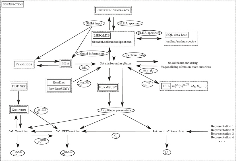
Figure 8: Flow chart of our numerical setup. The rectangular frames denote stand-alone program packages which are combined by gghXsection. It controls the flow of data (indicated by the ovals) among the individual components. More details are given in the text.

In the following we briefly describe the important features of our numerical program gghXsection. It consists of several components which take care of the generation of the spectrum, the computation of the Higgs boson mass, the convolution of the partonic cross sections with the PDFs in the effective theory and the determination of the best approximation for the three-loop matching coefficient. A flow chart showing the individual components can be found in Fig. 8.

• The individual components are called and controlled by the Mathematica program gghXsection.

• Our analytical expressions are parametrized in terms of $\overline{\rm DR}$ mass parameters defined at the renormalization scale $\mu_{R}$. For an automated generation of the required MSSM parameter spectra within Mathematica we use our own Mathematica package LHSQLDB. This package works as interface between Mathematica and the SUSY spectrum generators following the “Les Houches Accord” [48, 49] like SOFTSUSY [50], Spheno [51] or Suspect [52] (we use SOFTSUSY as default spectrum generator throughout this paper). Furthermore it is able to connect Mathematica to an SQL data base where SUSY spectra can be automatically saved to and/or loaded from, avoiding multiple recalculations of already known parameters.

  Since this package might be of general use, a separate publication is planned. However, a private version can be obtained from the authors upon request.

• We define the strong coupling constant in five-flavour QCD using the $\overline{\rm MS}$ scheme. The numerical results for $\alpha_{s}^{(5)}(\mu_{R})$ are taken from the PDF sets.

• The spectrum generator also provides input for H3m [53, 31] which is used to compute the light MSSM Higgs boson mass to three-loop accuracy. H3m uses FeynHiggs [54] for the two-loop expressions.

  Note that the spectrum generators can in general only be used for renormalization scales as low as the $Z$ boson mass. However, in our numerical analyses also lower scales appear since we choose $\mu_{s}=M_{h}/2$ as a central value. For this reason we have implemented the renormalization group equations (taken from Ref. [55]) ourselves in order to obtain the spectrum for all desired values of $\mu_{s}$ (see the program RunMSUSY in Fig. 8).

• In order to compute the $\overline{\rm DR}$ top quark mass from the on-shell one we use the results of Ref. [56, 57] which are based on the program TSIL. For this step we need the strong coupling constant in the full theory which we obtain with the help of RunDec [58, 59] and the extension of the decoupling and running routines to supersymmetry based on Refs. [60, 40].

• The integrations needed for the computation of $\Sigma$ are performed with the help of the self-written C++ program Xsection.

  The SM part entering our numerical analysis is based on results obtained in Ref. [18]. It is used to extract the quantities $\Sigma^{(i)}$ in Eq. (3.1) which are necessary to construct the top sector result up to NNLO.

• In the C++ program we have also included the computation of $\sigma_{tb}^{\rm SQCD}(\mu_{s})|_{\rm NLO}$ which is based on the formulae provided in Refs. [23, 19]. The analytic expressions for the amplitudes which we implemented in our numerical program are taken from Ref. [19] for the bottom and from Ref. [23] for the top sector which provides the SUSY QCD corrections up to NLO. Thus the exact bottom quark mass dependence is taken into account as well as the top quark, gluino and squark dependence in the effective-theory approach, i.e. in the formal limit $M_{h}\to 0$. For Higgs boson masses considered here this approximation approaches the exact result to high accuracy [15, 16, 17, 18]. We have cross checked our implementation against the results implemented in [20] in certain limits.

• We use LO, NLO and NNLO PDFs by the MSTW2008 collaboration [61] in order to obtain the respective predictions for $\sigma^{\rm SQCD}$ in Eq. (3.1). The choice of the PDFs determines the values of $\alpha_{s}(M_{Z})\equiv\alpha_{s}^{(5)}(M_{Z})$:

  $$\alpha_{s}^{\rm LO}(M_{Z}) = 0.1394\,,~{}\alpha_{s}^{\rm NLO}(M_{Z})=0.1202\,,~{}\alpha_{s}^{\rm NNLO}(M_{Z})=0.1171\,.$$ (36)

  The appropriate $\overline{\rm MS}$ beta function then determines $\alpha_{s}(\mu_{R})$ that enters the formulae.

• The procedure for the calculation of the best three-loop approximation of $C_{1}$ within SQCD as described in Subsection 2.3 is implemented in Mathematica.

• The electroweak correction which enter the final result in factorized form (cf. Eq. (3.1)) are taken from Ref. [46].

• If not stated otherwise the following default values are used:

  $$\mu_{s}=\frac{M_{h}}{2}\,, \mu_{h}=M_{t}\,, M_{t}=173.3~{}\mbox{GeV}\,.$$ (37)

3.3 Prediction to NNLO

In order to discuss the numerical effects we start with the $m_{h}^{\rm max}$ scenario introduced in Ref. [62]. The low-energy parameters are given by

$$A_{t}=A_{b}=A_{\tau}=\sqrt{6}\,m_{\rm susy}+\frac{\mu_{\rm susy}}{\tan\beta}\,, \mu_{\rm susy}=200~{}\mbox{GeV}\,, m_{\rm susy}=1000~{}\mbox{GeV}\,$$

$$M_{1}=5s_{W}^{2}/(3c_{W}^{2})M_{2}\,, M_{2}=200~{}\mbox{GeV}\,, M_{3}=800~{}\mbox{GeV}\,,$$ (38)

where the mass of the pseudo-scalar Higgs boson $M_{A}$ and the ratio of the vacuum expectation values of the two Higgs doublets $\tan\beta$ is varied. In Eq. (38) $A_{t}$ is the trilinear coupling, $\mu_{\rm susy}$ is the Higgs-Higgsino bilinear coupling from the super potential, $m_{\rm susy}$ is the common mass value for all squarks, $M_{1}$, $M_{2}$ and $M_{3}$ are the gaugino mass parameters and $s_{W}$ and $c_{W}$ are the sine and cosine of the weak mixing angle. The parameters in Eq. (38) are defined at the scale $\mu_{R}=\sqrt{m_{\rm susy}^{2}+M_{t}^{2}}$.

(a)	(b)

Figure 9: (a) $\sigma_{t}^{\rm SQCD}(\mu_{s},\mu_{h})$ and (b) $\sigma_{\rm full}$ as a function of $M_{A}$ and $\tan\beta$ in the $m_{h}^{\rm max}$ scenario.

In Fig. 9 we discuss the dependence of the cross section on $\tan\beta$ and $M_{A}$, the remaining parameters are fixed to the values of Eq. (38). The NNLO prediction for the top sector contribution $\sigma_{t}^{\rm SQCD}(\mu_{s},\mu_{h})$ is shown in Fig. 9(a) where the numbers on the contour lines correspond to the cross section in pb. $M_{A}$ is varied between 100 GeV and 200 GeV and we choose $\tan\beta\leq 20$. The (red) hyperbola-like lines indicate Higgs boson masses of 123 GeV (lower) and 129 GeV, respectively. Thus the area in between is in accordance with the result reported by ATLAS [1] and CMS [2]. The NNLO cross section has been obtained with the help of hierarchy (h1) which is appropriate since the SUSY mass spectrum is almost degenerate.

For comparison we show in Fig. 9(b) the complete result including also bottom quark effects and the electroweak corrections according to Eq. (3.1). One observes a significant enhancement of the cross section for small values of $M_{A}$ and large $\tan\beta$ (i.e. in the upper left corner). In the remaining parts of the plot only a reduction of a few percent is observed which comes basically from the destructive interference of the top and bottom contribution. Let us mention that a large part of the parameter space shown in Fig. 9 is already excluded experimentally which will be discussed below. Basically only the lower right part of the plot is experimentally still allowed. Note that this region is dominated by the contribution from the top sector and the bottom contribution only plays a minor role.

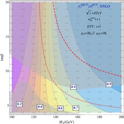
(a)	(b)

Figure 10: (a) NNLO $K$ factor corresponding to the prediction in Fig. 9(b). Panel (b) shows the ratio of the MSSM and the SM NNLO prediction from the top quark/top squark sector.

The effect of higher order corrections is conveniently parametrized in terms of the $K$ factor which we define through

$$K = \frac{\sigma^{\rm HO}}{\sigma^{\rm LO}}\,.$$ (39)

In Fig. 10(a) we show the NNLO (i.e. HO=NNLO in Eq. (39)) $K$ factor for the same parameter space as in Fig. 9. In the experimentally allowed region it amounts to about 100% where about 70% arise from the NLO corrections. It is interesting to compare the MSSM prediction to the one of the SM which is done in Fig. 10(b) where the ratio of the NNLO predictions in the two models is plotted. One observes that the supersymmetric corrections reduce the cross section by typically 60% to 90% in the parameter space where the Higgs boson mass is between 123 GeV and 129 GeV. Note, however, that for $M_{A}\;\hbox to0.0pt{\lower 3.5pt\hbox{$\mathchar 0\relax\sim$}\hss}\raise 1.0pt\hbox{$>$}\;140$ GeV this effect basically results from a modification of the Higgs couplings to fermions and thus is already present at LO. In fact for this region the $K$ factors in the SM and MSSM are very similar for the $m_{h}^{\rm max}$ scenario. In Fig. 10(b) we also show the regions excluded by searches performed at LEP [63] and CMS [64] which is indicated by the gray area.

The reason for the small deviations between the SM and MSSM in the $m_{h}^{\rm max}$ scenario is the heavy supersymmetric mass spectrum resulting from the input parameters in Eq. (38). Actually, the typical squark mass is 1000 GeV with only small differences between the individual flavours and the gluino mass takes the value $m_{\tilde{g}}=860$ GeV.

In the following we slightly modify the parameters in such a way that one of the top squarks becomes light whereas the other remains heavy. Thus, on one hand one obtains sizeable supersymmetric contributions to the Higgs boson production cross section and at the same time a Higgs boson mass which is sufficiently heavy. To date such a scenario has not been excluded by experimental searches.

In our modified $m_{h}^{\rm max}$ scenario the default values of the low-energy parameters are given by

$$A_{b}=A_{\tau}=2469.48~{}\mbox{GeV}\,, A_{t}=1500~{}\mbox{GeV}\,, \mu_{\rm susy}=200~{}\mbox{GeV}\,,$$

$$M_{1}=5s_{W}^{2}/(3c_{W}^{2})M_{2}\,, M_{2}=200~{}\mbox{GeV}\,, M_{3}=800~{}\mbox{GeV}\,,$$

$$m_{\rm susy}=1000~{}\mbox{GeV}\,, \tilde{m}_{t}=400~{}\mbox{GeV}\,,$$

$$M_{A}=1000~{}\mbox{GeV}\,, \tan\beta=20\,,$$ (40)

where $\tilde{m}_{t}$ represents the singlet soft SUSY breaking parameter of the right-handed top squark (i.e. EXTPAR 46 in the “Les Houches Accord” notation [48, 49]).

(a)

(b)

Figure 11: (a) Top squark masses and (b) lightest Higgs boson mass as a function of $\tilde{m}_{t}$ for the parameters given in Eq. (38).

In Fig. 11(a) we show the top squark masses as a function of $\tilde{m}_{t}$. The variation of this parameter essentially changes $m_{\tilde{t}_{1}}$ whereas $m_{\tilde{t}_{2}}$ remains almost constant at a large value of about 1050 GeV. For large values of $\tilde{m}_{t}$ one obtains a heavy spectrum and thus the supersymmetric corrections to the Higgs boson production become small. On the other hand, for a small value of $\tilde{m}_{t}$ and thus a large splitting in the top squark sector the numerical effect can be large as we will discuss below. The hierarchy in the top squark sector suggests to use (h2) for evaluating the three-loop corrections to $C_{1}$.

It is interesting to have a closer look at the numerical values of the three-loop coefficient $c_{1}^{(2)}$. For $\tilde{m}_{t}=400$ GeV we have $c_{1}^{(2)}(\mu=M_{t})\approx-0.58(1)$ and $c_{1}^{(2)}(\mu=M_{h}/2\approx 63~{}\mbox{GeV})\approx-14.66(1)$ and for $\tilde{m}_{t}=600$ GeV one obtains $c_{1}^{(2)}(\mu=M_{t})\approx 5.70(1)$ and $c_{1}^{(2)}(\mu=M_{h}/2\approx 63~{}\mbox{GeV})\approx-1.29(23)$. One observes a quite strong dependence of $c_{1}^{(2)}$ on the renormalization scale which demonstrates the importance of the three-loop calculation. Note that the renormalization scale dependence is compensated by the other quantities entering formula (3.1) for the cross section.

In order to get a feeling about the physical masses we list in the following the $\overline{\rm DR}$ mass values for the squark and gluino masses. For $\mu_{R}=M_{t}$ and $\tilde{m}_{t}=400$ GeV one obtains from the parameters provided by SOFTSUSY the following values

$$m_{\tilde{t}_{1}}=370~{}\mbox{GeV}\,, m_{\tilde{t}_{2}}=1045~{}\mbox{GeV}\,,$$

$$m_{\tilde{q}}=1042~{}\mbox{GeV}\,, m_{\tilde{g}}=860~{}\mbox{GeV}\,,$$ (41)

where $m_{\tilde{q}}$ corresponds to the average of $m_{\tilde{u}}$, $m_{\tilde{d}}$, $m_{\tilde{s}}$ and $m_{\tilde{c}}$.

The lightest MSSM Higgs boson mass $M_{h}$ as predicted from the parameters in Eq. (38) is shown in Fig. 11(b) where $\tilde{m}_{t}$ is varied in the same range as before. In this figure we compare $M_{h}$ as computed by SOFTSUSY (dashed lines) to the one obtained by H3m [53, 31] (solid line). Note that the latter, which includes three-loop corrections, is more than 1 GeV above the former. As one can see, in the whole range of $\tilde{m}_{t}$ the prediction remains within the horizontal lines which mark 123 GeV and 129 GeV, respectively, the limits motivated by the recent results reported by ATLAS [1] and CMS [2].

Figure 12: The cross section $\sigma_{t}^{\rm SQCD}(\mu_{s},\mu_{h})$ as a function of $\tilde{m}_{t}$ using the parameters in Eq. (38) to LO (bottom), NLO (middle) and NNLO (top). The dotted line corresponds to the SM and the dashed and solid lines to the MSSM.

In Fig. 12 we show $\sigma_{t}^{\rm SQCD}(\mu_{s},\mu_{h})$ as a function of $\tilde{m}_{t}$ at LO, NLO and NNLO (from bottom to top). For each order three curves are shown where the dotted curve corresponds to the SM. The SQCD corrections are included in the dashed and solid line where for the former the soft and hard scale have been identified with $M_{h}/2$ and for the latter $\mu_{s}=M_{h}/2$ and $\mu_{h}=M_{t}$ has been chosen. As already mentioned above, the difference between the SM and MSSM corrections is small for large values of $\tilde{m}_{t}$, for smaller values, however, a sizeable effect is visible. For example, for $\tilde{m}_{t}=400$ GeV a reduction of the cross section of about 5% is observed.

The difference between the dashed and solid line quantifies the effect of the resummation discussed in Subsection 3.1. It is negligible for large $\tilde{m}_{t}$, however, for smaller values it can be as large as 2-3%. It is interesting to note that supersymmetric three-loop corrections to $C_{1}$ computed in this paper play an important role. In case the three-loop coefficient is identified with the SM one a reduction of only 3% and not 5% is observed.

Figure 13: Renormalization scale dependence of the cross section $\sigma_{t}^{\rm SQCD}(\mu_{s}=\mu_{h})$.

In Fig. 13 we fix $\tilde{m}_{t}=400$ GeV and discuss the renormalization scale dependence of the LO, NLO and NNLO result by varying $\mu_{h}=\mu_{s}$ between 25 GeV and about 400 GeV. The SM (dotted) and the MSSM (solid lines) curves show a very similar behaviour. Close to the central scale $\mu_{s}=M_{h}/2$ one observes a crossing of the NNLO and NLO curves, i.e., vanishing NNLO corrections. It is at a slightly higher value for the MSSM which can be explained by the larger masses in the spectrum entering the predictions.

Figure 14: Lightest Higgs boson mass as a function of $\tan\beta$ for the parameters given in Eq. (40).

In a next step we study the dependence on $\tan\beta$ for fixed $\tilde{m}_{t}=400$ GeV. One observes top squark masses which are almost constant and are given by $m_{\tilde{t}_{1}}\approx 370$ GeV and $m_{\tilde{t}_{2}}\approx 1040$ GeV. On the other hand there is a strong dependence of $M_{h}$ on $\tan\beta$ which is shown in Fig. 14 for the result from SOFTSUSY and H3m. As one can see, for $\tan\beta\leq 6$ the predicted Higgs boson mass is below 123 GeV using H3m; on the basis of SOFTSUSY this boundary is reached already for $\tan\beta\approx 9$.

Figure 15: The cross section $\sigma_{t}^{\rm SQCD}(\mu_{s},\mu_{h})$ as a function of $\tan\beta$ using the parameters in Eq. (40) to LO (bottom), NLO (middle) and NNLO (top). The dotted line corresponds to the SM and the dashed and solid lines to the MSSM.

In Fig. 15 we show $\sigma_{t}^{\rm SQCD}(\mu_{s},\mu_{h})$ as a function of $\tan\beta$ for $5\leq\tan\beta\leq 30$ at LO, NLO and NNLO (from bottom to top) choosing $A_{t}=1500$ GeV and $\tilde{m}_{t}=400$ GeV. The SM result is again shown as dotted line. The MSSM predictions are both shown for $\mu_{h}=\mu_{s}=M_{h}/2$ (dashed) and $\mu_{h}=M_{t}$ and $\mu_{s}=M_{h}/2$ (solid line). As compared to the SM prediction the MSSM results are again reduced by a few percent. Note that this effect increases when going from LO to NLO and finally to NNLO where a difference of about 5% is observed. It is also interesting to mention that the proper choice of scales is not negligible: the results for $\mu_{h}=\mu_{s}$ are in general a few percent above the ones with $\mu_{h}\not=\mu_{s}$.

(a)

(b)

Figure 16: The cross section $\sigma^{\rm SQCD}(pp\to h+X)$ as a function of (a) $\tilde{m}_{t}$ and (b) $\tan\beta$ using the parameters in Eq. (40).

Let us finally present results for $\sigma(pp\to h+X)$ which include in addition bottom quark contributions up to NLO and furthermore also electroweak corrections. In Fig. 16(a) and (b) the dependence on $\tilde{m}_{t}$ and $\tan\beta$ is plotted, respectively, where from bottom to top the LO, NLO and NNLO results are shown. We refrain from showing the bottom quark contributions separately since they are about two orders of magnitude smaller than the top contributions. However, the interference terms have a visible effect which can be seen by the difference between the dashed and dotted curves since in the latter the quantities $\sigma_{tb}^{\rm SQCD}(\mu_{s})|_{\rm NLO}$ and $\sigma_{t}^{\rm SQCD}(\mu_{s})|_{\rm NLO}$ in Eq. (3.1) are set to zero. One observes a reduction of about 5% after including bottom quark effects — basically independent of $\tilde{m}_{t}$ and $\tan\beta$. Thus even for $\tan\beta=20$ the bottom quark effects are small for the considered scenarios and hence a NNLO calculation for $m_{b}\not=0$ is not mandatory. The reduction from top/bottom interference is to a large extend compensated by the electroweak corrections taken into account in a multiplicative way (cf. Eq. (3.1)) as can be seen by solid line which includes all contributions of Eq. (3.1).

4 Conclusions

We have computed the three-loop corrections to the matching coefficient of the effective Higgs-gluon coupling $C_{1}$ originating from supersymmetric QCD. The three-loop integrals contain several mass scales and thus an exact calculation on the basis of the techniques available these days is not possible. We have developed an approximation method based on expansions in mass hierarchies and mass differences which selects the best parametrization for the expansion parameters. The described procedure is not bound to the problem at hand but can certainly also be applied to other processes.

The three-loop result for $C_{1}$ is used in order to evaluate the Higgs boson production cross section at LHC to NNLO. Whereas the three-loop expressions are only available for vanishing light quark masses we include up to NLO the contributions from the top and bottom sector allowing for a non-vanishing bottom quark mass. Numerical results for the total production cross section are presented for a center-of-mass energy of $\sqrt{s}=8$ TeV for two MSSM scenarios which predict a light supersymmetric Higgs boson mass in accordance with the recent results from ATLAS and CMS. We study both the dependence on the renormalization scale, $\tan\beta$ and on the $\tilde{m}_{t}$, the singlet soft SUSY breaking mass parameter of the right-handed top squark. For the case where all supersymmetric masses are above 1 TeV the supersymmetric corrections are small. However, in case one of the top squarks becomes of the order of a few hundred GeV the supersymmetric corrections to the matching coefficient $C_{1}$ are not negligible any more and a sizeable effect on the production cross section is noticeable. For the scenarios considered in this paper a reduction of the NNLO prediction of the cross section by a few percent is observed. We also want to stress that visible effects result from separating the soft and hard scale in $C_{1}$ which automatically resums potentially large logarithms involving the Higgs boson mass.

In order to perform the numerical evaluation a flexible tool has been developed which allows a convenient handling of the spectrum generators in combination with Mathematica and C++ routines evaluating the cross sections. In a comfortable way it is possible to vary the renormalization scale or other parameters entering the prediction.

References

- [1] ATLAS Collaboration, arXiv:1207.7214.
- [2] CMS Collaboration, arXiv:1207.7235.
- [3] A. Pak, M. Steinhauser and N. Zerf, Eur. Phys. J. C 71 (2011) 1602 [arXiv:1012.0639 [hep-ph]].
- [4] S. Dittmaier, C. Mariotti, G. Passarino, R. Tanaka et al., [LHC Higgs Cross Section Working Group Collaboration], arXiv:1101.0593 [hep-ph].
- [5] S. Dittmaier, C. Mariotti, G. Passarino, R. Tanaka et al., [LHC Higgs Cross Section Working Group Collaboration], arXiv:1201.3084 [hep-ph].
- [6] H. M. Georgi, S. L. Glashow, M. E. Machacek and D. V. Nanopoulos, Phys. Rev. Lett. 40 (1978) 692.
- [7] A. Djouadi, M. Spira and P. M. Zerwas, Phys. Lett. B 264 (1991) 440.
- [8] S. Dawson, Nucl. Phys. B 359 (1991) 283.
- [9] M. Spira, A. Djouadi, D. Graudenz and P. M. Zerwas, Nucl. Phys. B 453 (1995) 17, arXiv:hep-ph/9504378.
- [10] R. V. Harlander and W. B. Kilgore, Phys. Rev. Lett. 88 (2002) 201801, arXiv:hep-ph/0201206.
- [11] C. Anastasiou and K. Melnikov, Nucl. Phys. B 646 (2002) 220, arXiv:hep-ph/0207004.
- [12] V. Ravindran, J. Smith and W. L. van Neerven, Nucl. Phys. B 665 (2003) 325, arXiv:hep-ph/0302135.
- [13] R. V. Harlander and K. J. Ozeren, Phys. Lett. B 679 (2009) 467 [arXiv:0907.2997 [hep-ph]].
- [14] A. Pak, M. Rogal and M. Steinhauser, Phys. Lett. B 679 (2009) 473 [arXiv:0907.2998 [hep-ph]].
- [15] R. V. Harlander and K. J. Ozeren, JHEP 0911 (2009) 088 [arXiv:0909.3420 [hep-ph]].
- [16] A. Pak, M. Rogal and M. Steinhauser, JHEP 1002 (2010) 025 [arXiv:0911.4662 [hep-ph]].
- [17] R. V. Harlander, H. Mantler, S. Marzani and K. J. Ozeren, arXiv:0912.2104 [hep-ph].
- [18] A. Pak, M. Rogal and M. Steinhauser, JHEP 1109 (2011) 088 [arXiv:1107.3391 [hep-ph]].
- [19] G. Degrassi and P. Slavich, JHEP 1011 (2010) 044 [arXiv:1007.3465 [hep-ph]].
- [20] R. V. Harlander, F. Hofmann and H. Mantler, JHEP 1102 (2011) 055 [arXiv:1012.3361 [hep-ph]].
- [21] C. Anastasiou, S. Beerli and A. Daleo, Phys. Rev. Lett. 100 (2008) 241806 [arXiv:0803.3065 [hep-ph]].
- [22] R. V. Harlander and M. Steinhauser, Phys. Lett. B 574 (2003) 258 [arXiv:hep-ph/0307346].
- [23] R. V. Harlander and M. Steinhauser, JHEP 0409 (2004) 066 [arXiv:hep-ph/0409010].
- [24] G. Degrassi and P. Slavich, Nucl. Phys. B 805 (2008) 267 [arXiv:0806.1495 [hep-ph]].
- [25] M. Muhlleitner, H. Rzehak and M. Spira, arXiv:1001.3214 [hep-ph].
- [26] M. Muhlleitner and M. Spira, Nucl. Phys. B 790 (2008) 1 [arXiv:hep-ph/0612254].
- [27] R. Bonciani, G. Degrassi and A. Vicini, JHEP 0711 (2007) 095 [arXiv:0709.4227 [hep-ph]].
- [28] R. Harlander and M. Steinhauser, Phys. Rev. D 68 (2003) 111701 [arXiv:hep-ph/0308210].
- [29] A. Kurz, M. Steinhauser and N. Zerf, arXiv:1206.6675 [hep-ph].
- [30] A. I. Davydychev and J. B. Tausk, Nucl. Phys. B 397 (1993) 123.
- [31] P. Kant, R. V. Harlander, L. Mihaila and M. Steinhauser, JHEP 1008 (2010) 104 [arXiv:1005.5709 [hep-ph]].
- [32] W. Siegel, Phys. Lett. B 84 (1979) 193.
- [33] R. V. Harlander, D. R. T. Jones, P. Kant, L. Mihaila and M. Steinhauser, JHEP 0612 (2006) 024 [arXiv:hep-ph/0610206].
- [34] R. Harlander, P. Kant, L. Mihaila and M. Steinhauser, JHEP 0609 (2006) 053 [arXiv:hep-ph/0607240].
- [35] I. Jack, D. R. T. Jones, P. Kant and L. Mihaila, JHEP 0709 (2007) 058 [arXiv:0707.3055 [hep-th]].
- [36] T. Hermann, L. Mihaila and M. Steinhauser, Phys. Lett. B 703 (2011) 51 [arXiv:1106.1060 [hep-ph]].
- [37] K. G. Chetyrkin, B. A. Kniehl and M. Steinhauser, Nucl. Phys. B 510 (1998) 61, arXiv:hep-ph/9708255.
- [38] http://www-ttp.particle.uni-karlsruhe.de/Progdata/ttp12/ttp12-26/
- [39] A. Bednyakov, A. Onishchenko, V. Velizhanin and O. Veretin, Eur. Phys. J. C 29 (2003) 87 [hep-ph/0210258].
- [40] A. Bauer, L. Mihaila and J. Salomon, JHEP 0902 (2009) 037 [arXiv:0810.5101 [hep-ph]].
- [41] V. A. Smirnov, “Applied asymptotic expansions in momenta and masses,” Springer Tracts Mod. Phys. 177 (2002) 1.
- [42] A. V. Bednyakov, Int. J. Mod. Phys. A 22 (2007) 5245 [arXiv:0707.0650 [hep-ph]].
- [43] D. Eiras and M. Steinhauser, Nucl. Phys. B 757 (2006) 197 [hep-ph/0605227].
- [44] N. Zerf, “Dreischleifenkorrekturen zur Higgsbosonproduktion durch Gluonfusion im MSSM” (PhD thesis, KIT, 2012). http://digbib.ubka.uni-karlsruhe.de/volltexte/1000026537
- [45] S. P. Martin, In *Kane, G.L. (ed.): Perspectives on supersymmetry II* 1-153 [hep-ph/9709356].
- [46] S. Actis, G. Passarino, C. Sturm and S. Uccirati, Phys. Lett. B 670 (2008) 12, arXiv:0809.1301 [hep-ph].
- [47] C. Anastasiou, R. Boughezal and F. Petriello, JHEP 0904 (2009) 003 [arXiv:0811.3458 [hep-ph]].
- [48] P. Z. Skands, B. C. Allanach, H. Baer, C. Balazs, G. Belanger, F. Boudjema, A. Djouadi and R. Godbole et al., JHEP 0407 (2004) 036 [hep-ph/0311123].
- [49] B. C. Allanach, C. Balazs, G. Belanger, M. Bernhardt, F. Boudjema, D. Choudhury, K. Desch and U. Ellwanger et al., Comput. Phys. Commun. 180 (2009) 8 [arXiv:0801.0045 [hep-ph]].
- [50] B. C. Allanach, Comput. Phys. Commun. 143 (2002) 305 [arXiv:hep-ph/0104145].
- [51] W. Porod, Comput. Phys. Commun. 153 (2003) 275 [hep-ph/0301101].
- [52] A. Djouadi, J. -L. Kneur and G. Moultaka, Comput. Phys. Commun. 176 (2007) 426 [hep-ph/0211331].
- [53] R. V. Harlander, P. Kant, L. Mihaila and M. Steinhauser, Phys. Rev. Lett. 100 (2008) 191602 [Phys. Rev. Lett. 101 (2008) 039901] [arXiv:0803.0672 [hep-ph]].
-
[54]
M. Frank, T. Hahn, S. Heinemeyer, W. Hollik, H. Rzehak and G. Weiglein,
JHEP 0702 (2007) 047
[hep-ph/0611326];
http://www.feynhiggs.de/. - [55] L. V. Avdeev, D. I. Kazakov and I. N. Kondrashuk, Nucl. Phys. B 510 (1998) 289 [hep-ph/9709397].
- [56] S. P. Martin, Phys. Rev. D 72, 096008 (2005) [arXiv:hep-ph/0509115].
- [57] S. P. Martin and D. G. Robertson, Comput. Phys. Commun. 174 (2006) 133 [hep-ph/0501132].
- [58] K. G. Chetyrkin, J. H. Kühn and M. Steinhauser, Comput. Phys. Commun. 133 (2000) 43, arXiv:hep-ph/0004189.
- [59] B. Schmidt and M. Steinhauser, Comput. Phys. Commun. 183 (2012) 1845 [arXiv:1201.6149 [hep-ph]].
- [60] R. Harlander, L. Mihaila and M. Steinhauser, Phys. Rev. D 72 (2005) 095009 [arXiv:hep-ph/0509048].
- [61] A. D. Martin, W. J. Stirling, R. S. Thorne and G. Watt, Eur. Phys. J. C 63 (2009) 189 [arXiv:0901.0002 [hep-ph]].
- [62] M. S. Carena, S. Heinemeyer, C. E. M. Wagner and G. Weiglein, Eur. Phys. J. C 26 (2003) 601 [hep-ph/0202167].
- [63] S. Schael et al. [ALEPH and DELPHI and L3 and OPAL and LEP Working Group for Higgs Boson Searches Collaborations], Eur. Phys. J. C 47 (2006) 547 [hep-ex/0602042].
- [64] S. Chatrchyan et al. [CMS Collaboration], Phys. Lett. B 713 (2012) 68 [arXiv:1202.4083 [hep-ex]].
- [65] P. Uwer, arXiv:0710.2896 [physics.comp-ph].