From the CMD of $\omega$ Centauri and (super-)AGB stellar models to a Galactic plane passage gas purging chemical evolution scenario

Abstract

We have investigated the color-magnitude diagram of $\omega$ Centauri and find that the blue main sequence (bMS) can be reproduced only by models that have a of helium abundance in the range $Y=0.35$–$0.40$. To explain the faint subgiant branch of the reddest stars (“MS-a/RG-a” sequence), isochrones for the observed metallicity ([Fe/H] $\approx-0.7$) appear to require both a high age ($\sim 13$ Gyr) and enhanced CNO abundances ([CNO/Fe] $\approx 0.9$). $Y\approx 0.35$ must also be assumed in order to counteract the effects of high CNO on turnoff colors, and thereby to obtain a good fit to the relatively blue turnoff of this stellar population. This suggest a short chemical evolution period of time ($<1$ Gyr) for $\omega$ Cen. Our intermediate-mass (super-)AGB models are able to reproduce the high helium abundances, along with [N/Fe] $\sim 2$ and substantial O depletions if uncertainties in the treatment of convection are fully taken into account. These abundance features distinguish the bMS stars from the dominant [Fe/H] $\approx-1.7$ population. The most massive super-AGB stellar models ($M_{\rm ZAMS}\geq 6.8\,{\rm M}_{\odot}$, $M_{\mathrm{He,core}}\geq 1.245\,{\rm M}_{\odot}$) predict too large N-enhancements, which limits their role in contributing to the extreme populations. In order to address the observed central concentration of stars with He-rich abundance we show here quantitatively that highly He- and N-enriched AGB ejecta have particularly efficient cooling properties. Based on these results and on the reconstruction of the orbit of $\omega$ Cen with respect to the Milky Way we propose the galactic plane passage gas purging scenario for the chemical evolution of this cluster. The bMS population formed shortly after the purging of most of the cluster gas as a result of the passage of $\omega$ Cen through the Galactic disk (which occurs today every $\sim 40\mathrm{Myrs}$ for $\omega$ Cen) when the initial-mass function of the dominant population had “burned” through most of the Type II supernova mass range. AGB stars would eject most of their masses into the gas-depleted cluster through low-velocity winds that sink to the cluster core due to their favorable cooling properties and form the bMS population. In our discussion we follow our model through four passage events, which could explain not only some key properties of the bMS, but also of the MS-a/RGB-a and the $s$-enriched stars.

1. Introduction

Omega Centauri provides an especially valuable constraint on our understanding of chemical evolution because of its unusual properties and its proximity, which enables us to study its component stellar populations in great detail over a very extended range in luminosity. While it has been known for some time that the giants in this system encompass a range in [Fe/H] from $\sim-2.2$ to $-0.5$ (e.g. Brown & Wallerstein, 1993; Suntzeff & Kraft, 1996), the extensive spectroscopic surveys carried out in the past decade, in particular (Smith et al., 2000; Hilker et al., 2004; Kayser et al., 2006; van Loon et al., 2007; Johnson et al., 2008; Johnson & Pilachowski, 2010; Marino et al., 2012, and references therein), have established that the metallicity distribution rises sharply from [Fe/H] $\approx-2.2$ to a strong peak at [Fe/H] $\approx-1.7$, with a long tail that drops off to higher metal abundances containing secondary peaks at [Fe/H] $\approx-1.4$, $-1.1$, and $-0.7$. Type Ia supernovae appear to have contributed to the chemical makeup of only the most metal-rich stars given that their measured [$\alpha$/Fe] abundance ratios are significantly reduced from the constant value of $\approx 0.35$ found in stars having [Fe/H] $<-0.8$ (Pancino et al., 2002; Origlia et al., 2003). The elevated $\alpha$-element abundances over most of the range in metallicity (also see Kayser et al.) implies that Type II supernovae were the major producers of these elements. Moreover, the rapid rise in the [La/Fe] ratio between the most metal-deficient and the [Fe/H] $>-1.5$ populations (by a factor of 3 according to Johnson & Pilachowski) indicates that $s$-processing, and therefore, intermediate-mass asymptotic-giant branch (AGB) stars contributed significantly to the chemistry of $\omega$ Cen after the dominant [Fe/H] $=-1.7$ population had formed.

Accompanying these spectroscopic advances have been equally impressive improvements in the photometric data. The detailed, and deep, color-magnitude diagrams (CMDs) derived by Lee et al. (1999); Hughes & Wallerstein (2000); Rey et al. (2004); Bedin et al. (2004); Sollima et al. (2005a, 2007a); Villanova et al. (2007); Calamida et al. (2009), and Bellini et al. (2009, 2010), among others, have also established the existence of several discrete stellar populations in $\omega$ Cen. The most baffling one of them is a so-called “blue main sequence” (bMS), discovered by (Anderson, 1997), that is clearly separated from, and bluer at a given magnitude than, the MS associated with the dominant [Fe/H] $\approx-1.7$ population (see the CMDs reported by, e.g., Bedin et al. and Villanova et al.). What has made this discovery so puzzling is the determination by Piotto et al. (2005) that the former is more metal rich than the latter by $\approx 0.3$ dex. As discussed by Piotto et al., and anticipated by Bedin et al.  and Norris (2004), the most obvious (only?) way to reconcile these observations with stellar evolutionary theory is to infer that the bMS stars have unusually high helium abundances ($Y>0.35$).

Although it has not yet been possible to make a definitive connection of the bMS through the subgiant region of the CMD to the RGB (but see King et al., 2012), Johnson & Pilachowski (2010) have found that the giants in their sample with “extreme” abundances (i.e., those with low C and O, together with high N, Na, and Al; see their Fig. 23) constitute a similar proportion of all giants ($\approx 27\%$) as the fraction of all MS stars that are located on the bMS. Furthermore, since (for the most part) their radial distributions are quite similar, it is tempting to conclude that the aforementioned giants are the descendants of stars that had occupied the bMS earlier in their evolutionary history. However, because the O-poor stars do not exhibit a correlation with [La/Fe], while the O-rich stars do, and because there is no apparent correlation of the La abundance with radius, in contrast to the observed trend for the O-poor stars, Johnson & Pilachowski suggest that the observed light element abundances reflect both (i) the retention by $\omega$ Cen of the ejecta of AGB stars and (ii) in situ mixing on the RGB.

There is a second feature of the CMD that is potentially quite challenging to explain, and that is the extension of the reddest giant branch (independently discovered by Lee et al. (1999) and by Pancino et al. (2000), who gave it the name “RGB-a” that has since been used to refer to it), through the subgiant branch (Ferraro et al., 2004) to very faint magnitudes on the MS (Bellini et al., 2010). Because this is is the most metal-rich of the discrete populations that have been identified, it is presumably also the youngest one. Consequently, its age provides a key constraint on the timescale over which most of the chemical evolution took place in $\omega$ Cen. Because the turnoff of this fiducial sequence is so faint, the age of this stellar population must be quite old, implying that the bulk of the star formation occurred over a rather short interval of time. Indeed, the reason why some investigations (e.g. Hilker et al., 2004; Rey et al., 2004) derived an extended star formation history ($\sim 3$–4 Gyr) in their analyses is that they had mistakenly adopted a bright turnoff for the RGB-a population. However, it remains unclear whether the different stellar populations of $\omega$ Cen have the same age to within a few $\times 10^{8}$ yr (D’Antona et al., 2011a; Valcarce & Catelan, 2011), or they span a range in age of $\mathrel{\hbox{\raise 2.58334pt\hbox{$<$}\kern-7.74998pt\lower 2.15277pt\hbox{$\sim$}}}2$ Gyr (Sollima et al., 2005a) or as much as 3–5 Gyr (Stanford et al., 2006; Villanova et al., 2007).

Among stellar evolution models of different mass ranges, intermediate-mass and super-AGB stars have been proposed as the source of the He-enriched and otherwise extreme abundance patterns associated with the bMS. However, models of these types of stars do not always reproduce the required high He, high N, and low O abundance associated with the bMS in a quantitative way. For example, the intermediate-mass AGB models by Ventura & D’Antona (2009, specifically the $Z=6\times 10^{-4}$ case that is applicable to the first, most metal-deficient generation in $\omega$ Cen) predict $Y=0.329$ and [N/Fe]$=1.84$ for $M_{\rm ZAMS}=5.0\,\,{\rm M}_{\odot}$ and $Y=0.360$ and [N/Fe]$=1.36$ for $M_{\rm ZAMS}=6.0\,\,{\rm M}_{\odot}$. The super-AGB models by Ventura & D’Antona (2011) produce a maximum ejecta He abundance of $Y=0.36$, but information for N is not available. The envelope He abundance at the end of the second dredge-up in the super-AGB models by Siess (2007) reach $0.37$ for non-overshooting models, and $0.38$ for models with core overshooting. Siess (2010) do not provide a model for $Z=6\times 10^{-4}$, but interpolating between their super-AGB thermal pulse calculations for $Z=0.001$ and $Z=10^{-4}$ yield He mass fractions in the ejecta of $Y\sim 0.33$, while N is enhanced by a factor of $10$ to $100$. Moreover, those models with the largest increases in the nitrogen abundance also have the smallest O depletion, and models with O depletions of $\sim 1\,\mathrm{dex}$ have N enhancements of only $\sim 1\,\mathrm{dex}$. While existing models clearly point qualitatively in the right direction, it is not clear to us what it would take to reproduce the “extreme” abundance mixtures that are associated with the bMS in $\omega$ Cen in a quantitative sense.

Producing He-abundances in intermediate-mass AGB ejecta that exceeds the He-abundance of the “extreme” abundance mix in any significant way appears to be very difficult within model calculations. This does not leave a lot of room (if any) for dilution of the AGB ejecta before the formation of the blue main-sequence stars. Dilution has been suggested, however, in order to reproduce the abundance anti-correlations (D’Ercole et al., 2008). We are considering here rather the origin and evolution of one sub-population at a time. The presentation of Na-O abundances by sub-populations identified with a four-criterion cluster analysis by Gratton et al. (2011, Fig. 6) rather suggests that the anti-correlation is the result of the superposition of discrete Na and O abundance in different sub-populations, and as we will argue later (Sect. 5.2) dilution may not be needed. We therefore investigate the evolution of first-generation intermediate-mass AGB and super-AGB stars with the goal to generate the “extreme” abundance mix without taking into account any dilution.

In any case, the AGB ejecta may preferentially converge in the cluster center via AGB cooling flows (D’Antona et al., 2011b, and refs. there). Such gas may have to be isolated, for example through supernova-induced clearing of intracluster gas that is ejected from stars having initial masses outside the range that encompasses intermediate-mass AGB and super-AGB stars (Conroy & Spergel, 2011), while the tidal stripping of old stars increases the ratio of second- to first-generation stars (Bekki, 2011). However, complete SN gas purging makes it difficult to envisage how a spread in [Fe/H], like that observed in $\omega$ Cen, is produced.

The present study has been undertaken to address some of the issues described above. In §2, newly computed sets of isochrones and zero-age horizontal branch (ZAHB) loci for different values of $Y$, $Z$, and heavy-element mixtures are compared with the CMD of $\omega$ Cen in order to illustrate how the interpretation of the observations would be affected by the assumed variations in the chemical abundances, and to make some assessment of the age and helium content of the stars that belong to the bMS and MS-a components. §3 investigates under which assumptions the predicted yields from $>5\,{\rm M}_{\odot}$ AGB stars can be made to agree with the observed/inferred high $Y$, high-N, low-O abundances. Finally, a short summary of the main results of this study is given in §4, which also discusses in some detail how our stellar evolutionary results together with the efficient cooling properties of the ejecta from intermediate-mass AGB stars may naturally explain the formation of additional populations like the bMS. A key point in our proposed scenario is the periodic purging of the gas from globular clusters (or dwarf galaxies) that is expected to occur throughout their evolutionary histories whenever their orbits cause them to pass through the Galactic plane. Implications of this scenario are briefly summarized in §5.

2. Color-Magnitude Diagram Considerations

Several grids of stellar evolutionary tracks were computed using a significantly updated version of the Victoria code (VandenBerg et al., 2012) which now treats the diffusion of helium (but not the metals) as well as extra mixing below envelope convection zones (when they exist) using methods very similar to those described by Proffitt & Michaud (1991). All of the model computations reported in this study assumed a value of $\alpha_{\rm MLT}=2.007$ for the usual mixing-length parameter, so as to satisfy the solar constraint when the mix of heavy elements derived for the Sun by Asplund et al. (2009) is assumed. The abundances of the individual $\alpha$-elements in this mixture were increased by approximately the amounts found in very metal-deficient stars according to Cayrel et al. (2004), resulting in the “standard” metals mix (see the second column of Table 1) that applies to normal Population II stars, including (presumably) the dominant [Fe/H] $\approx-1.7$ component of $\omega$ Cen.

Table 1Chemical Abundance Ratios

	[m/Fe]
m	Standard	Extreme	$\omega$ Cen	NGC 2808
eC	$+$0.0	$-0.7$	$-0.5$	$-0.7$
eN	$+$0.0	$+2.0$	$+1.5$	$+2.0$
eO	$+0.5$	$-0.5$	$-0.5$
Ne	$+0.3$	$+$0.0
Na	$+$0.0	$+0.8$	$+0.6$	$+0.8$
Mg	$+0.3$	$+$0.0		$+0.1$
Al	$+$0.0	$+1.1$	$+1.1$	$+1.1$
Si	$+0.4$	$+0.4$	$+0.4$
eP	$+$0.0	$+$0.0
eS	$+0.3$	$+0.3$
Cl	$+$0.0	$+$0.0
Ar	$+0.3$	$+0.3$
eK	$+$0.0	$+$0.0
Ca	$+0.3$	$+0.3$	$+0.3$	$+0.3$
Ti	$+0.3$	$+0.3$	$+0.3$
Cr	$+$0.0	$+$0.0
Mn	$+$0.0	$+$0.0
Ni	$+$0.0	$+$0.0

The third column of Table 1 lists the “extreme” heavy-element mixture that has been assumed in some of the comparisons of observations with models to be discussed shortly. Remarkably, multiple main sequences have also been discovered in NGC 2808 Piotto et al. (2007), and the chemical abundances derived by Bragaglia et al. (2010) for one of its bluest MS stars appear to be quite similar to those found in what are believed to be the red-giant descendants of bMS stars in $\omega$ Cen (compare the entries in the 4th and 5th columns). To maximize the impact of these abundance anomalies on the predicted properties of stellar models, we have chosen to adopt the largest of the [$m$/Fe] values (in an absolute sense) that have been determined for $\omega$ Cen and NGC 2808 in our “extreme” heavy-element mix (column 3). However, we note that, although Marino et al. (2011) have found that the [O/Fe] value varies from $-0.6$ to $+0.9$ at metallicities appropriate to bMS stars, the [CNO/Fe] ratio spans the relatively small range of $\approx+0.4$–$0.7$ (see Marino et al., 2012). This suggests that the CNO abundances listed in the third column of Table 1 are somewhat more extreme than those found in $\omega$ Cen stars having [Fe/H] $\approx-1.5$. On the other hand, Marino et al. (2012, see their Fig. 3) find that the [CNO/Fe] value ranges between $+0.7$–$0.9$ at [Fe/H] $\sim-1.0$, and as discussed below, such high values appear to be necessary to explain the faint subgiant branch of the MS-a/RG-a population.

Also worth mentioning is the fact that opacity data for both mixtures were generated using the code described by Ferguson et al. (2005) for the low-temperature regime, while complemetary high-temperature tables (similar to those reported by Iglesias & Rogers, 1996) were obtained via the OPAL website. Note, as well, that the interpolation program developed by P. Bergbusch, which is similar to that described by VandenBerg et al. (2006), but with the significant improvements (see VandenBerg et al., 2012), was used to produce all of the isochrones considered in this investigation.

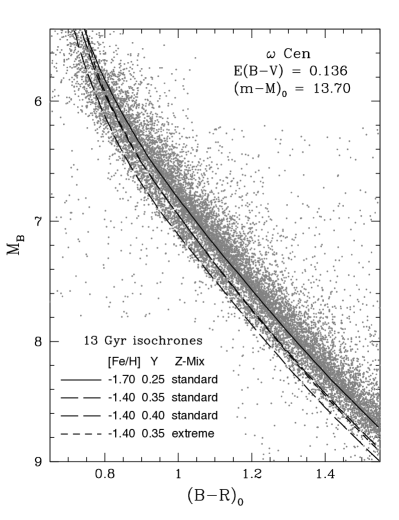
Figure 1.— Comparison of the lower main-sequence extensions of isochrones for the indicated age and chemical abundances with the photometry of $\omega$ Cen reported by Sollima et al. (2007a). The adopted values of $E(B-V)$ and the true distance modulus are noted in the upper right-hand corner.

To begin our analysis, we first compare, in Fig. 1, the main-sequence segments of several isochrones with the lower MS photometry of $\omega$ Cen given by Sollima et al. (2007a), based on VLT FORS1 observations. The latter have been converted to the [$(B-R)_{0},\,M_{B}$]-plane assuming $(m-M)_{0}=13.70$ (Bellazzini et al., 2004), $E(B-V)=0.136$ (Schlegel et al., 1998), and $A_{B}=4.07\,E(B-V)$, $A_{R}=2.44\,E(B-V)$ (McCall, 2004). Bellazzini et al. have argued that the Lub (2002) determination of $E(B-V)=0.11\pm 0.01$ mag is the current best estimate of the foreground reddening, and that may well be the case. However, the main purpose of Fig. 1 is to determine the value of $Y$ that is needed to reproduce the location of the bMS stars relative to the main sequence of the dominant [Fe/H] $\approx-1.7$ population. One could obviously adopt the lower value of $E(B-V)$ and then increase the predicted $B-R$ colors by 0.026 mag to obtain an identical fit of the models to the observations in a differential sense. In fact, fainter than $M_{B}=6.5$, the synthetic colors had to be adjusted by $\delta(B-R)=0.02(M_{B}-6.5)$ in order for the [Fe/H] $=-1.70$, $Y=0.25$ isochrone (the solid curve) to accurately reproduce the observed MS over the entire magnitude range that has been ploteed. (Such a color offset could arise if, among other possibilities, the MARCS model atmospheres predict too much flux at short wavelengths or there are systematic errors in the model $T_{\rm eff}$ scale due to the treatment of convection or the surface boundary conditions.)

When such a color correction is applied (to all of the model loci), one finds that the bMS stars in $\omega$ Cen are bracketed by isochrones for $Y=0.35$ and $Y=0.40$ (the long-dashed curves) on the assumption of the observed [Fe/H] value ($-1.4$, Piotto et al., 2005) and the “standard” Pop. II metals mixture. (We note that $Y=0.39\pm 0.02$ has been obtained by (King et al., 2012) from a fit of isochrones to their improved CMD.) Indeed, these results are fully consistent with the findings of Piotto et al. (see their Fig. 7) and Sollima et al. (2007a, their Fig. 9), who performed similar comparisons using completely independent theoretical computations. (While we have opted to plot 13 Gyr isochrones, mainly because their extensions to brighter magnitudes are shown in a subsequent figure, the location of the lower MS is obviously independent of the assumed age.) Interestingly, fainter than $M_{B}\sim 5.7$, isochrones for the “standard” and the “extreme” heavy-element mixtures are essentially identical when the same values of $Y$ and [Fe/H] are assumed (compare the short-dashed curve with the long-dashed curve for the same helium abundance). (Of course, differences would be evident if photometric filters are used that are sensitive to the abundances of CNO and/or other heavy elements; see, e.g. Bellini et al., 2010; Sbordone et al., 2011; Milone et al., 2012) As others, including those mentioned above and e.g., Norris (2004), have concluded, it does not appear to be possible to explain the location of the bMS stars in $\omega$ Cen (and NGC 2808) without invoking high $Y$ — provided that, indeed, chemical abundance differences are primarily responsible for the CMD anomalies. Indeed, we explored the impact of varying the abundances of O, Mg, and Si using isochrones presented by VandenBerg et al. (2012), which allow for variations in the abundances of several metals in turn, but we were unable to find a satisfactory alternative explanation (i.e., other than high $Y$) for the location of the bMS relative to the main-sequence fiducial of the dominant [Fe/H] $\sim-1.7$ population.

There is one aspect of Fig. 1 that deserves further comment. The bMS stars are clearly separated from the dominant red MS at $6.7<M_{B}<7.7$, but not at lower luminosities, where the two populations appear to merge. By contrast, the isochrones remain parallel to one another over the entire range in $M_{B}$ that is considered. One can speculate that this may be a color–$T_{\rm eff}$ relations effect; i.e., that at sufficiently cool temperatures, stars having the “extreme” metals mixture are redder at a fixed $T_{\rm eff}$ and gravity than stars having normal Pop. II abundances. To investigate this possibility, it would be necessary to compute proper model atmospheres and synthetic spectra for the two heavy-element mixtures and then compute the fluxes in the various filter passbands. Additional work along these lines would certainly be worthwhile.

Figure 2.— Comparison of several ZAHB loci for the indicated properties with the horizontal-branch stars in $\omega$ Cen having $M_{B}<3.2$ (from Bellini et al., 2009) on the assumption of the reddening and distance modulus that were assumed in the previous figure, as noted. As mentioned in the text, the predicted colors had to be increased by $+0.04$ mag in order for the models to reproduce the HB population in the blue tail satisfactorily.

Before turning to an examination of the upper-MS to lower-RGB stars in $\omega$ Cen, it is instructive to examine its HB population. Fig. 2 compares the HB stars that have $M_{\rm F435W}<3.2$ from the published Bellini et al. (2009) HST data set with ZAHB loci that have been calculated for indicated values of [Fe/H] and $Y$, using the numerical methods described by VandenBerg et al. (2000). As indicated, the same reddening and distance modulus that were assumed in the previous figure have been adopted here, along with $A_{\rm F435W}=4.081\,E(B-V)$ and $A_{\rm F625W}=2.637\,E(B-V)$ from Sirianni et al. (2005). However, besides the reddening adjustment, the predicted colors had to be corrected by $+0.04$ mag in order to achieve a satisfactory fit of the ZAHB loci to the steeply sloped blue stars. It is not clear why an additional zero-point correction is needed, as the same ZAHBs appear to provide an excellent match to the $F606W,F814W$ observations of Anderson et al. (2008) without having to apply any ad hoc color shift. Be that as it may, this concern is not of particular importance for the present analysis, given that we are primarily interested in the comparison of predicted and observed CMDs in a differential sense. Note that, to accomplish the transformation of the models to the observed plane, we have used the color–$T_{\rm eff}$ relations applicable to ACS photometry that were presented by Bedin et al. (2005), and kindly provided to us by S. Cassisi (2011, priv. communication).

As already shown by Sollima et al. (2005b), most of the HB stars in $\omega$ Cen having $(m_{\rm F435W}-m_{\rm F625W}>0.0$ appear to be matched quite well by ZAHB loci for [Fe/H] values from $\sim-1.7$ to $\sim-1.4$ and $Y\approx 0.25$ (the short-dashed curves). Although some of the observed stars lie between the two solid curves, which represent ZAHBs for [Fe/H] $=-1.4$ and $Y=0.30,0.35$, it is not obvious whether they truly have higher helium abundances or they have simply evolved to their current CMD locations from initial structures on ZAHBs for lower values of $Y$. The most noteworthy result of Fig. 2 is the lack of any stars brighter or bluer than the ZAHBs for $Y=0.35$ and [Fe/H] $=-1.4$ — assuming either the “standard” or the “extreme” metals mixtures (i.e., the brightest of the solid curves and the long-dashed curve, respectively). ZAHB loci for lower [Fe/H] values and/or higher helium abundances would be even brighter at a given color than the latter. Thus, if $\omega$ Cen does contain stars having $Y>0.35$, they must evolve to ZAHB locations well down the blue tail. This would perhaps not be too surprising given that, at the same age and [Fe/H] value, the turnoff mass is predicted to be $\approx 0.12$ solar masses less for stars having $Y=0.35$ than those for $Y=0.25$, nearly independently of the metals mixture that is assumed. If similar, and significant, amounts of mass loss occur on the RGB, then stars having high $Y$ should evolve into ZAHB structures that are much hotter than those for normal helium abundances. This has already been appreciated by a number of others (e.g. Busso et al., 2007; D’Antona & Caloi, 2008), and in fact, Cassisi et al. (2009) have suggested that the densely populated clump of HB stars at $m_{F435W}\sim 18.6$ ($M_{F435W}\sim 4.4$) in the $\omega$ Cen CMD may be He-rich stars.

Fig. 3 makes a number of interesting comparisons of theoretical isochrones with the Bellini et al. (2009) ACS data for upper-MS, subgiant, and lower-RGB stars of $\omega$ Cen. (Only a fraction of the total number of observed stars have been plotted, for the sake of improved clarity.) Curiously, it was not necessary to apply any correction to the isochrone colors, as derived from the transformations by Bedin et al. (2005), in order to obtain quite a good match to the observed MS stars, which leads us to wonder whether the difficulty noted above concerning the colors of ZAHB models should be attributed to a small problem with these color–$T_{\rm eff}$ relations (for just warm stars) or whether our interpretation of the observed HB is incorrect. The former explanation would seem to be the most likely one given that, if the predicted colors are not adjusted to the red, the core He-burning stars of $\omega$ Cen would lie below, or redward, of all of the ZAHB loci (assuming that the adopted distance modulus is accurate), which would be very difficult to explain.

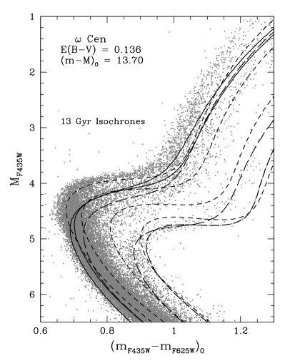
Figure 3.— Comparison of 13 Gyr isochrones with the upper main-sequence, subgiant, and lower red-giant-branch populations of $\omega$ Cen. The short-dashed curves assume $Y=0.25$, the “standard” mix of heavy elements (see Table 1), and [Fe/H] $=-1.7$, $-1.4$, $-1.0$, and $-0.7$, in the direction from left to right. The solid curves were computed for [Fe/H] $=-1.4$ and the same metals mix, but for $Y=0.35$ and 0.40: the isochrone for the higher helium abundance has a bluer turnoff. The long-dashed loci represent isochrones for $Y=0.35$, the “extreme” mix, and [Fe/H] $=-1.4$ and $-0.7$, in the direction from left to right. The dot-long-dashed isochrone assumes the “extreme” mixture, as well, but a normal helium abundance ($Y=0.250$).

The short-dashed curves represent 13 Gyr isochrones for $Y=0.25$, and [Fe/H] $=-1.7$, $-1.4$, $-1.0$, and $-0.7$ (in the direction from left to right), on the assumption of the “standard” metals mix. (An isochrone for the lowest metallicity and an age of 12.5 Gyr would actually provide the closest match to the densest distribution of stars which define the brightest subgiant branch (SGB), and is therefore our best estimate of the age of the most metal-poor population of $\omega$ Cen.) The RGB segments of these isochrones appear to be too red, by $\sim 0.05$ mag, which suggests that either the model $T_{\rm eff}$ scale is somewhat too cool and/or the adopted color transformations for low-gravity stars are slightly too red. However, in a relative sense, the difference in the colors of the predicted RGBs for [Fe/H] $=-1.7$ and $-1.0$, at a fixed color, is comparable to the observed width of the main distribution of giant stars.

Isochrones represented by the solid curves and the bluest of the long-dashed loci extend to higher luminosities the same isochrones that were plotted in Fig. 1. As emphasized by Sollima et al. (2005b), among others, variations in the helium content have only minor effects on the luminosity and morphology of the SGB. This is demonstrated by the fact that the two solid isochrones (for $Y=0.35$ and 0.40) and the short-dashed isochrone (for $Y=0.25$) — all of which were computed for [Fe/H] $=-1.4$ on the assumption of the “standard” mix of heavy elements — are nearly coincident along the subgiant branch. On the other hand, the isochrones for $Y=0.35$ and [Fe/H] $=-1.4$ that has been computed for the “extreme” metals mix (the aforementioned long-dashed isochrone) has a significantly fainter SGB at a same age (due to these models having a much higher [CNO/Fe] abundance ratio).

Although King et al. (2012) have found that the SGB tentatively identified as the extension of the of the bMS can be matched by isochrones for high Y and a normal $\alpha$-enhanced mixture, the sensitivity of subgiant luminosities, at a fixed age, to the total abundance of the CNO elements (e.g., see Cassisi et al., 2008), clearly complicates the determination of the ages of $\omega$ Cen SGB stars if derived from their locations relative to theoretical isochrones for different metallicities (e.g., Hilker et al., 2004; Stanford et al., 2007). In order to have robust ages, even in a differential sense, it is of critical importance to take into account any star-to-star variations that exist in both [Fe/H] and [CNO/Fe]. According to Marino et al. (2012), the mean [CNO/Fe] ratio varies from $\approx 0.25$ at [Fe/H] $=-1.9$ to $\approx 0.75$ at [Fe/H] $=-1.0$ (which is very difficult to understand; see their discussion of this point), with a dispersion of about 0.2 to 0.4 dex at a given metallicity. Such variations of [CNO/Fe] at a fixed iron abundance will affect predicted ages at the level of $\sim 0.6$–1.3 Gyr (VandenBerg et al., 2012).

Finally, Fig. 3 shows that the most metal-rich of the discrete stellar populations in $\omega$ Cen has a fainter SGB, and an appreciably bluer turnoff, than those of a 13 Gyr isochrone for $Y=0.25$ and [Fe/H] $=-0.7$ (“standard” mix). Surprisingly, the reddest of the long-dashed isochrones, for $Y=0.35$ and [Fe/H] $=-0.7$ (“extreme” mixture), does reproduce these observations quite well — though the inferred value of $Y$ cannot be determined very precisely because the upper MS and turnoff of the MS-a population is not very well defined in the photometry that we have used. On the other hand, isochrones for the same metallicity and a normal helium content ($Y=0.25$) are clearly too red and they fail to reproduce the slope of the subgiant branch (note the location of the dot-long-dashed curve). Isochrones for high $Y$ do not suffer from such difficulties. Thus, it appears to be a fairly robust stellar evolution prediction that the MS-a/RG-a stars have high CNO and He abundances.

These results support previous suggestions. In particular, Marino et al. (2011) noted that “as with bMS stars, the colors and the metallicity of the MS-a are consistent with being populated by He-rich stars (Norris, 2004; Bellini et al., 2010). Moreover, based on observations taken in many different ACS bandpasses, the aforementioned Bellini et al. paper suggested that this population has “peculiar” CNO abundances. Indeed, the predicted age of the MS-a/RG-a stars will be less than the age of the universe only if they have high CNO abundances (assuming that our estimate of the $\omega$ Cen distance is accurate). Furthermore, the slope of the subgiant branch, which is well defined in Fig. 3, can be reproduced by the models only if high $Y$ is also assumed. As far as our contention that a high helium abundances is needed to match the turnoff color is concerned, we note that (i) the $T_{\rm eff}$ scale of our models agrees well with that derived for solar neighborhood stars (having Hipparcos parallaxes) over the entire range in [Fe/H] encompassed by them (see VandenBerg et al., 2010), and (ii) isochrones for close to the primordial abundance of helium and standard Pop. II metal abundances provide a good fit to the [Fe/H] $=-1.7$ population. Stellar models should be quite reliable in a differential sense.

Our CMD analysis suggests that the different stellar populations in $\omega$ Cen have close to the same age, and hence that the chemical evolution in this system must have occurred over a relatively short period of time ($\mathrel{\hbox{\raise 2.58334pt\hbox{$<$}\kern-7.74998pt\lower 2.15277pt\hbox{$\sim$}}}1$ Gyr). (For the MS-a/RG-a stars to be appreciably younger than the universe, they they would neeed to have a higher [Fe/H] value and/or higher CNO or helium abundances than those assumed in the best-fit isochrone.) Especially intriguing is the very real possibility that the most metal-rich component has a high helium abundance. Is there, then, a connection between these stars and the bMS? Before offering some suggestions on how the chemical evolution in $\omega$ Cen may have proceeded (in §4), we will first examine whether the chemical yields from AGB models that form out of gas having the “standard” mix of heavy elements (column 2 of Table 1) will be similar to the “extreme” mixture (col. 3).

3. AGB and super-AGB stellar evolution with uncertain convective mixing physics

Our analysis of the CMD of $\omega$ Cen suggests that somehow out of the first, and dominant, [Fe/H] $\approx-1.7$ population, in which the metals have the “standard” $\alpha$-enriched distribution, at least two distinguishable new stellar populations have been generated. These are the [Fe/H] $\approx-1.4$ bMS stars and their counterparts on the RGB, which appear to have helium abundances between $Y=0.35$ and $0.40$, and the so-called “MS-a/RG-a” population at an even higher Fe abundance ($\approx-0.7$) that seems to have a similarly enhanced He abundance as well as enhanced C$+$N$+$O, judging from the comparison of isochrones with the observed photometry.

In this section we wish to address the question of whether current AGB and/or super-AGB models are able to produce ejecta out of which the bMS population, and possibly the MS-a population, can form.

3.1. Model assumptions

We have calculated several intermediate-mass AGB and super-AGB stellar evolutionary sequences with an initial abundance distribution (see Table 2) that closely resembles the abundances found in the dominant generation of stars at [Fe/H] $\approx-1.7$. The tabulated mass-fraction abundances for the metals are, in fact, equivalent to the abundances that have been labelled as the “standard” mix in Table 1, and the adopted isotopic ratios are from Asplund et al. (2009).

We use the MESA stellar evolution code (rev. 2941, Paxton et al., 2011). The MESA paper by Paxton et al. already contains verification cases for a wide range of stellar evolution cases, including thermal pulses and dredge-up in AGB stars. In addition, we have now also run massive AGB models with the same initial abundances and similar enough physics assumptions as those chosen for the grid of models including massive AGB stars by Herwig (2004b) obtained with the EVOL stellar evolution code, and we find the MESA results again to be in reasonable agreement.

We adopt a customized nuclear network (identified as sagb_NeNa.net), which is based on the MESA network agb.net. To be more specific, we consider 23 chemical species (including the major isotopes) for the elements from H to Na, ending with ${}^{24}\mathrm{Mg}$, as well as the $pp$-chain, the CNO cycles, the NeNa cycle, He-burning, the ${}^{13}\mathrm{C}(\alpha,\mathrm{n})^{16}\mathrm{O}$ reaction, and the ${}^{12}\mathrm{C}+\mbox{${}^{12}\mathrm{C}$}\rightarrow^{20}\mathrm{Ne}+\alpha$ reaction. The nuclear reaction rates have been taken from the NACRE compilation (Angulo et al., 1999).

Table 2Initial abundance distribution for the AGB stellar evolution calculations.

Isotope	Initial mass fraction
${}^{1}\mathrm{H}$	$0.7494$
${}^{2}\mathrm{H}$	$1.4576\times 10^{-5}$
${}^{3}\mathrm{He}$	$2.3547\times 10^{-5}$
${}^{4}\mathrm{He}$	$0.2500$
${}^{7}\mathrm{Li}$	$4.6251\times 10^{-1}$
${}^{12}\mathrm{C}$	$4.7392\times 10^{-5}$
${}^{13}\mathrm{C}$	$5.7061\times 10^{-7}$
${}^{14}\mathrm{N}$	$1.4014\times 10^{-5}$
${}^{15}\mathrm{N}$	$3.2165\times 10^{-8}$
${}^{16}\mathrm{O}$	$3.6666\times 10^{-4}$
${}^{17}\mathrm{O}$	$1.3930\times 10^{-7}$
${}^{18}\mathrm{O}$	$7.3508\times 10^{-7}$
${}^{19}\mathrm{F}$	$2.5000\times 10^{-9}$
${}^{22}\mathrm{Ne}$	$4.6817\times 10^{-5}$
${}^{21}\mathrm{Ne}$	$1.1223\times 10^{-7}$
${}^{22}\mathrm{Ne}$	$3.4425\times 10^{-6}$
${}^{23}\mathrm{Na}$	$5.9273\times 10^{-7}$
${}^{24}\mathrm{Mg}$	$7.1662\times 10^{-5}$
Z	$5.9030\times 10^{-4}$

For the mixing-length parameter we adopt $\alpha_{\mathrm{MLT}}=1.73$, which is obtained from a standard solar model. MESA is executed in hydrodynamic mode and sufficient artificial viscosity is assumed in order to damp out the large velocities that are otherwise predicted to occur near the surface during the advanced stages of AGB thermal-pulse (TP) evolution (especially during the dredge-up phase). In addition to the default mesh-point controls, we refine the mesh using the abundances of $\mathrm{p}$, ${}^{4}\mathrm{He}$, ${}^{13}\mathrm{C}$ and ${}^{14}\mathrm{N}$ so that the chemical abundance profiles are always well resolved. Additional criteria have been implemented in order to improve the resolution of He-shell flashes and the advance of the thin H-burning shell during the interpulse phase as a function of time. We use the atmosphere option ’simple_photosphere’, and we assume a mass-loss rate of $\log\dot{M}\ \mathrm{(in\,{\rm M}_{\odot}/\,\mathrm{yr})}\approx-4.8$ to $-4.3$, which is obtained using the Blöcker (1995) mass-loss rate that has been incorporated in MESA with $\eta=5\times 10^{-4}$. (Although some sequences were followed for up to 100 TPs, none of the model stars had lost significant amounts of mass by the time the calculations were terminated.) We also adopt the OPAL opacities that include C- and O-enhanced tables (Iglesias & Rogers, 1996). In the pre-AGB evolution we consider convective boundary mixing (CBM) according to the exponential CBM model (Freytag et al., 1996; Herwig et al., 1997; Herwig, 2000), with $f=0.014$ at all convective boundaries.

We have chosen initial masses of $5.0\,{\rm M}_{\odot}$ and $7.0\,{\rm M}_{\odot}$ to represent, in turn, an intermediate-mass AGB star having a CO core and a hydrogen-free core mass of $M_{\rm H}=0.991\,{\rm M}_{\odot}$ at the first TP, and a super-AGB star with an ONe core and a hydrogen-free core mass of $M_{\rm H}=1.2677\,{\rm M}_{\odot}$ at the first TP. We present below the results that have been obtained for these two cases when both standard and modified assumptions are made about stellar interior mixing processes.

3.2. Intermediate-mass AGB star model

3.2.1 Standard mixing assumption

We will first describe the surface abundance evolution of the standard 5$\,{\rm M}_{\odot}$ calculation and how it relates to the evolution of convection zones in some detail (Fig. 4). For the standard case, we assume convective boundary mixing with $f_{\mathrm{ce}}=0.004$ at the bottom of the convective envelope and $f_{\mathrm{pdcz}}=0.002$ at the bottom of the pulse-driven convection zone. Both of these values are much smaller than those normally assumed in computations of low-mass AGB models. As shown by Herwig (2005) a CBM parameter as large as indicated by $s$-process-constraints in low-mass AGB stars ($f_{\mathrm{ce}}\sim 0.13$) would lead to very vigorous hot dredge-up which eventually evolves into a corrosive flame penetrating deeper and deeper into the core. The model evolution is soon terminated in this case due to high mass loss induced by extreme luminosities. Such a scenario seems incompatible with the requirements for the ejecta of intermediate-mass and super AGB stars in $\omega$ Cen. This issue does, however, highlight shortcomings regarding our present models of CBM in the deep stellar interior.

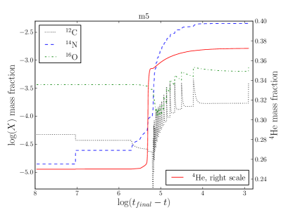
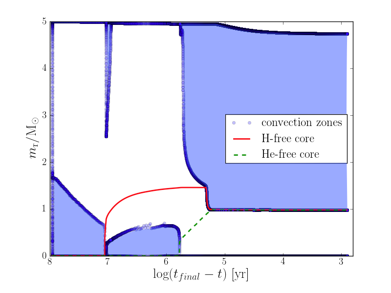
Figure 4.— Surface abundance evolution of dominant CNO isotopes and ${}^{4}\mathrm{He}$ of 5$\,{\rm M}_{\odot}$ stellar evolution tracks with standard mixing assumptions (top panel) and Kippenhahn diagram (bottom panel). The time axis is reverse-logarthmic to accomodate the accelerating evolution, $t_{\mathrm{final}}=9.077424\times 10^{7}\,\mathrm{yr}$.

At the beginning of the evolution all chemical species have surface abundances that are unmodified from those listed in Table 2, and they do not change until the end of H-core burning. Then, at $\log(t_{\mathrm{final}}-t)=7$, the first dredge-up leads to a small decrease of the surface ${}^{12}\mathrm{C}$ abundance and a corresponding increase of the surface ${}^{14}\mathrm{N}$ abundance. No changes are predicted during He-core burning, after which major changes, again initially for ${}^{12}\mathrm{C}$ and ${}^{14}\mathrm{N}$ but then for ${}^{4}\mathrm{He}$. They are the result of the second dredge-up, which starts at $\log(t_{\mathrm{final}}-t)=5.7$ and ends at $5.25$. The second dredge-up, which takes place even before the first thermal pulse on the AGB, mixes into the envelope a large fraction of the He that was produced by H-shell burning during the He-core burning phase. This mixing event is responsible for a major increase in the surface He abundance, from initially $X(^{4}\mathrm{He})=0.250$ to $0.353$ for this case. By the end of the second dredge-up the ${}^{14}\mathrm{N}$ abundance has increased by $+0.6\mathrm{dex}$, ${}^{12}\mathrm{C}$ has decreased by $0.3\mathrm{dex}$ and ${}^{16}\mathrm{O}$ has decreased by $0.08\mathrm{dex}$.

These modifications of the surface, and therefore envelope composition, all point in the right direction, but quantitatively they are far from matching the “extreme” abundances listed in Table 1. However, further processing of the envelope takes place during the thermal-pulse AGB phase that starts shortly after the end of the second dredge-up. Individual TP-related mixing events, like the third dredge-up and the He-shell flash convection zones are fully resolved in the stellar evolution calculation, but not in the Kippenhahn plot shown in Fig. 4. However, for the 5$\,{\rm M}_{\odot}$ case, the repeated action of the third dredge-up after each thermal pulse is evident from the periodic step-like increase of the ${}^{12}\mathrm{C}$ and ${}^{16}\mathrm{O}$ surface abundance evolution, which is also shown in Fig. 4. The thermal-pulse AGB evolution starts at $\log(t_{\mathrm{final}}-t)=5.2$, and though little or no third dredge-up occurs during the five He-shell flashes, there is a steep initial increase of the ${}^{14}\mathrm{N}$ envelope abundance up to a mass fraction of $\log(X)=-3.0$ at $\log(t_{\mathrm{final}}-t)\sim 5.1$. This is due, at first, to the destruction of ${}^{16}\mathrm{O}$ when the third dredge-up is weak, and then to just the effects of deep third dredge-up (typically $\Delta m_{\mathrm{dup}}=1.7\times 10^{-3}\,{\rm M}_{\odot}$ per pulse) after each of the next six TPs, These events mix into the envelope primary ${}^{12}\mathrm{C}$ and ${}^{16}\mathrm{O}$ from He-shell burning. Note that, due to the hot dredge-up in our models (Herwig, 2004a), the immediate CN-cycling conversion of ${}^{12}\mathrm{C}$ to ${}^{14}\mathrm{N}$ during the dredge-up phase is responsible for approximately $20\%$ (a fraction that decreases to below $10\%$ in subsequent thermal pulses) of the ${}^{14}\mathrm{N}$ production per pulse cycle (also see Fig. 5 and the discussion below). Hot-bottom burning during the interpulse phase is responsible for the remainder of the ${}^{14}\mathrm{N}$ production from the transmutation of both ${}^{12}\mathrm{C}$ and ${}^{16}\mathrm{O}$ via the CNO cycle at the bottom of the convective envelope.

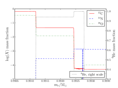
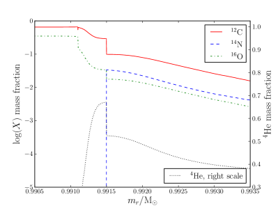
Figure 5.— Profile of CNO isotopes and ${}^{4}\mathrm{He}$ during the He-shell (approximately at the end of the first $1/3$ of the duration of the He-shell flash convection when the convection zone is still growing outward in mass) and during the third dredge-up (when $1.3\times 10^{-3}\,{\rm M}_{\odot}$ out of a total of eventually $1.9\times 10^{-3}\,{\rm M}_{\odot}$ have been dredged-up) following the He-shell flash.

At $\log(t_{\mathrm{final}}-t)=5.08$ after eleven TPs, of which the last six were followed by efficient dredge-up, the total ${}^{14}\mathrm{N}$ enhancement has risen to $1.83\,\mathrm{dex}$ and the envelope He abundance is $Y=0.356$. While the ${}^{14}\mathrm{N}$ abundance is now in reasonably good agreement with the estimate in the “extreme” abundance mixture, the value of $Y$ is just reaching the lower limit of the range that has been inferred from the isochrones. Furthermore, the O abundance has decreased by only $\sim 0.5\,\mathrm{dex}$ and the C abundance has increased in total by $\leq 0.3\,\mathrm{dex}$. These reductions are both significantly less than the values that define the “extreme” abundance distribution. However, for carbon, in particular, it should be kept in mind that the “extreme” composition is based in part on the measured abundances in RGB stars, which are known to experience extra-mixing processes (e.g. Denissenkov & VandenBerg, 2003) that cause the C abundance to decrease with increasing luminosity as they climb the giant branch (Gratton et al., 2000).

In the more advanced pulses (starting around the tenth TP), each dredge-up event will mix the entire intershell helium as well as a small layer interior to the bottom of the He-shell flash convection zone where $X(^{12}\mathrm{C})=0.63$ and $X(^{16}\mathrm{O})=0.35$. The dredge-up into and below the former He-shell flash convection zone is shown in Fig. 5. The He-shell flash the convection zone combines ${}^{12}\mathrm{C}$- and ${}^{16}\mathrm{O}$-rich material from deeper layers ($<0.9912\,{\rm M}_{\odot}$) with the ${}^{14}\mathrm{N}$-rich H-shell ashes (between $0.9924$ and $0.9927\,{\rm M}_{\odot}$). At the time that the profiles are shown the convection zone has not yet reached its full extent, which occurs when the upper boundary has approached the location of the former H-burning shell ($0.9927\,{\rm M}_{\odot}$). At this point the ${}^{12}\mathrm{C}$ and ${}^{16}\mathrm{O}$ mass-fraction abundances in the He-shell flash convection zone are $X(^{12}\mathrm{C})=0.046$ and $X(^{16}\mathrm{O})=0.012$, which is considerably lower than the typical intershell abundances in lower mass models.

After the end of the He-shell flash, the dredge-up (see the bottom panel of Fig. 5) proceeds into the H-free core. The profiles illustrate how ${}^{14}\mathrm{N}$ is produced in-situ as ${}^{12}\mathrm{C}$ streams through the hot convective boundary at $m_{\mathrm{r}}=0.9915\,\,{\rm M}_{\odot}$. In the outward direction, it is the simultaneous burning of ${}^{14}\mathrm{N}$ and the convective mixing in the envelope that causes the sloped chemical abundance profiles. The ${}^{4}\mathrm{He}$ abundance just below the convective boundary is reduced from the value obtained at earlier times (see the top panel) due to nuclear burning, which forms a small additional amount of ${}^{12}\mathrm{C}$ and ${}^{16}\mathrm{O}$ to be subsequently dredged-up. However, close inspection of the models shows that the bulk of the ${}^{12}\mathrm{C}$ and ${}^{16}\mathrm{O}$ that is mixed to the surface does not come from the region occupied by the former convective He-shell flash, but originates instead from the layer just beneath. The deepest mass coordinate reached by the third dredge-up in this event is $0.9908\,\,{\rm M}_{\odot}$. Therefore, the amount of ${}^{12}\mathrm{C}$ coming from the region below the former He-shell flash convection zone is $0.0003\,{\rm M}_{\odot}\ \times 0.63=1.8\times 10^{-4}\,{\rm M}_{\odot}$, which is approximately the same as the ${}^{12}\mathrm{C}$ content of the envelope at this point. Thus, the visible spikes in the ${}^{12}\mathrm{C}$ surface abundance evolution (Fig. 4) and much of the overall enhancement of CNO is due to deep dredge-up that reaches below the He-shell flash convection zone.

This deep dredge-up will also bring ${}^{16}\mathrm{O}$ from below the He-shell flash convection zone into the envelope. In this model the dredge-up of ${}^{16}\mathrm{O}$ outperforms the capacity of hot-bottom burning to reduce the ${}^{16}\mathrm{O}$ abundance in later TPs. As a result, this model predicts an increasing ${}^{16}\mathrm{O}$ abundance, which would eventually lead to an enhanced O abundance in the AGB wind ejecta compared with the initial O abundance. This is clearly in contradiction to the target abundance in the “extreme” mixture. While this deep dredge-up will also mix all of the He in the helium shell into the envelope, this contribution to the evolution of the envelope helium abundance is negligible. The bulk of the He comes from hot-bottom burning during the interpulse phase. During the 15 fully developed thermal pulses (i.e., not counting the first five TPs that have insignificant dredge-up) the He mass-fraction abundance increases by $\Delta Y=0.02$, reaching $0.372$ in the last computed model. Therefore, a value of $Y$ of $\approx 0.4$ could be obtained after another 21 thermal pulses, which is in all likelihood a very plausible scenario.

In conclusion, our standard intermediate-mass AGB stellar model is able to generate wind ejecta with He as well as N abundances in the ranges required by the “extreme” mixture. As a matter of fact, the total N enhancement according to our model is $2.5\,\mathrm{dex}$, which exceeds the enhancement specified in the “extreme” abundance distribution. However, it is possible to alter the abundances of C, N and O in the models by fine tuning (reducing) the convective boundary mixing (CBM) parameter at the bottom of the convective envelope. This may be necessary, in fact, given that there will be many more thermal pulses in a real star than we have computed here, with the consequence that the envelope enrichment would be stretched out over a much larger number of dredge-up events. However, because the ${}^{12}\mathrm{C}$ for the production of ${}^{14}\mathrm{N}$ during hot-bottom burning and ${}^{16}\mathrm{O}$ come from the same region in the star, it is not possible to obtain a significant N enhancement and, at the same time, a significant O reduction (to be consistent with the “extreme” abundance distribution) without further modifications of our model assumptions.

3.2.2 Increased mixing-length parameter

In addition to boundary mixing uncertainties, some assumptions need to be made about the mixing-length parameter, $\alpha_{\mathrm{MLT}}$, when modeling convection in the envelopes of AGB stars. It is commonly assumed that the value of $\alpha_{\mathrm{MLT}}$, as calibrated by fits to the solar parameters, can be applied universally to all convection zones during all evolutionary phases. However, both simulations as well as semi-empirical evidence suggest that the deep convection zones of giant envelopes, comprising essentially fully convective configurations, are better described by an increased mixing-length parameter. A variable (i.e., non-constant) $\alpha_{\mathrm{MLT}}$ parameter was already suggested by the radiation-hydrodynamics simulations by Ludwig et al. (1999), also see the later work by Robinson et al. (2004). Specifically relevant to giant stars, Porter & Woodward (2000) presented 3D-simulations of deep envelope convection that were best reproduced within the mixing-length picture if $\alpha_{\mathrm{MLT}}=2.68$, assuming the formulation of the MLT given in Cox & Giuli (1968). In addition, a semi-empirical determination of $\alpha_{\mathrm{MLT}}$ was obtained from the the modeling of the pulsation of highly-evolved, variable, intermediate-mass stars ($4-6\,{\rm M}_{\odot}$) in the LMC and SMC by McSaveney et al. (2007) when they derived spectroscopic abundances. For three giants, they determined significantly larger values of $\alpha_{\mathrm{MLT}}$, ranging from 2.2 to 2.4 — also based on the Cox & Giuli (1968) version of the MLT. Taken together, there is ample justification to explore the effects of assuming a larger value of $\alpha_{\mathrm{MLT}}$. Numerical experiments with enhanced values of $\alpha_{\mathrm{MLT}}$ have been carried out for intermediate mass AGB stars and super-AGB stars previously by Karakas et al. (2012) and Siess (2010, , using a post-processing code).

To investigate this issue, we have computed two evolutionary sequences starting at the first thermal pulse of the standard sequence that was described in the previous section. For the convective boundary mixing (CBM) parameters, we used $f_{\mathrm{ce}}=0.002$ and $f_{\mathrm{pdcz}}=0.001$, while at all other convective boundaries, we adopted $f=0.01$. One sequence had $\alpha_{\mathrm{MLT}}=1.73$, as assumed in the standard sequence, and the other had $\alpha_{\mathrm{MLT}}=2.40$. Both sequences were followed through the initial 5 to 6 TPs with no or little third dredge-up, and the computations were halted after another two full TP cycles with fully developed third dredge-ups had been completed. The evolutionary properties of the models over those two TP cycles are compared in Table 3. The $\alpha_{\mathrm{MLT}}=2.40$ calculations show, on average, higher interpulse H-burning, and peak-flash He-burning, luminosities. For the high-$\alpha_{\mathrm{MLT}}$ case, the third dredge-up is more than twice as deep, and it reaches below the bottom of the convection zone boundary established by the previous He-shell flash at the second fully developed dredge-up, as compared with the standard-$\alpha_{\mathrm{MLT}}$ case wherein the dredge-up proceeds into about two-thirds of the former He-shell convection zone. This standard-$\alpha_{\mathrm{MLT}}$ case predicts a shallower third dredge-up compared with the sequence described in Sect. 3.2.1 because the adopted value of $f_{\mathrm{ce}}$ is smaller.

The convection assumptions, primarily parameterized through $\alpha_{\mathrm{MLT}}$ and $f_{\mathrm{ce}}$, significantly alter the evolution of the envelope abundances. Over the first two pulses with significant dredge-up, the enhancement in the He abundance is a factor of $6.6$ higher for the $\alpha_{\mathrm{MLT}}=2.40$ case than in the models for $\alpha_{\mathrm{MLT}}=1.73$. Also, in the $\alpha_{\mathrm{MLT}}=1.73$ case, the increase in $\Delta X(^{4}\mathrm{He})$ per pulse at later times is consistent with the average value for $\Delta X(^{4}\mathrm{He})$ reported for the standard case in the previous section. Since, in a differential sense, the same is true for the $\alpha_{\mathrm{MLT}}=2.40$ case, we find that intermediate-mass AGB models with a larger value of the mixing-length produce He from hot-bottom burning more efficiently. Insofar as the CNO elements are concerned, the deeper dredge-up that occurs when $\alpha_{\mathrm{MLT}}=2.40$ means that significantly more C and O is brought into the envelope, even from below the former He-shell flash convection zone. However, the more efficient hot-bottom burning in the model with higher $\alpha_{\mathrm{MLT}}$ means that, not only is N produced efficiently, but even O is depleted efficiently. Over the first two pulses of the $\alpha_{\mathrm{MLT}}=2.40$ sequence, the O abundance is depleted by $\sim-0.6\,\mathrm{dex}$ in comparison with the initial abundance.

3.2.3 Conclusion

We conclude that, with the right combination of the convection model parameters $\alpha_{\mathrm{MLT}}$ and $f_{\mathrm{ce}}$, it should be possible, in principle, to account for He mass-fraction abundances up to $Y\sim 0.40$, as well as sufficiently enhanced N and depleted O, in the wind ejecta from intermediate-mass AGB stars. Indeed, to obtain the low oxygen abundances that have been observed, it seems to be necessary to adopt a high value of $\alpha_{\mathrm{MLT}}$. On the other hand, the increased effectiveness of third dredge-up that is also found when a larger value of $\alpha_{\mathrm{MLT}}$ is assumed, may lead to an enhancement of N that is too large for a given increase in $Y$. We have therefore constructed one additional $5\,{\rm M}_{\odot}$ stellar model sequence with $\alpha_{\mathrm{MLT}}=2.4$, but with a further reduction in the value of the $f_{\mathrm{ce}}$ parameter. This case has been evolved over ten thermal pulse cycles with fully developed dredge-up (see the top panel of Fig. 6). While the N enhancement now reaches $\sim 2\,\mathrm{dex}$ and the He abundance reaches the average value of the range that is indicated by fitting isochrones to the bMS, the O abundance has been depleted by about $1\,\mathrm{dex}$, just as required by the “extreme” abundance distribution. However, even this model sequence does not show a significant C depletion.

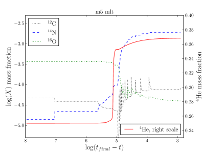
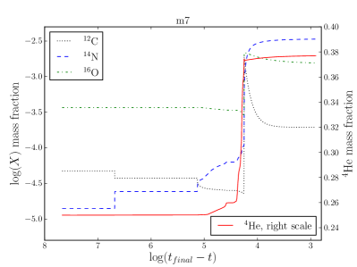
Figure 6.— Surface abundance evolution of 5$\,{\rm M}_{\odot}$ stellar evolution track with enhanced mixing-length parameter $\alpha_{\mathrm{MLT}}=2.4$ (top panel, $t_{\mathrm{final}}=9.1641578\times 10^{7}\,\mathrm{yr}$) and surface abundance evolution for 7$\,{\rm M}_{\odot}$ track with standard mixing assumption (bottom panel, $t_{\mathrm{final}}=4.6642752\times 10^{7}\,\mathrm{yr}$).

A real intermediate-mass AGB star will likely do more thermal pulses than we were able to compute here. This means either that the real star may have convection properties that will stretch out the chemical abundance modifications seen in our stellar models over more thermal pulses, or that the ejecta of the AGB star are more extreme in their abundance patterns than indicated by the “extreme” metals mixture, which would leave some room for the dilution of the ejected winds with unprocessed “standard” abundances before forming the bMS generation of stars. As discussed earlier the “extreme” abundance mix may in fact be an upper limit for the bMS in $\omega$ Cen, and a somewhat less extreme abundance mix in this cluster would add to the possibility of dilution.

With these caveats in mind, it seems very reasonable to conclude that intermediate-mass AGB star models are capable of producing abundance patterns very similar to that listed in Table 1 under the column heading “extreme”.

3.3. Super-AGB model

For somewhat higher initial masses, stars have a core mass at the first thermal pulse which is larger than approximately $1.05\,{\rm M}_{\odot}$, in which case, C burning is ignited and those stars will form a ONeMg core (García-Berro & Iben, 1994). These are the so-called “super-AGB” stars, which, like their intermediate-mass AGB star counterparts with CO cores, have periodic thermal pulses, dredge-up events, and hot-bottom burning. It has been suggested that these super-AGB stars could provide the chemically peculiar ejecta that are required in order for a stellar population like the bMS in $\omega$ Cen to form.

3.3.1 Deep second dredge-up mixing in the $7\,{\rm M}_{\odot}$ case

We have calculated stellar evolution sequences with an initial mass of $7\,\,{\rm M}_{\odot}$ that adopt the same initial abundances, and employ the same physical assumptions, as in the $5\,{\rm M}_{\odot}$ sequence discussed above, but explore uncertainties in convection assumptions.

In Fig. 6 we show the evolution of the surface abundances for our standard case. As reported for the lower mass models in Sect. 3.2.1, the chemical composition changes as a result of the first dredge-up (at $\log(t_{\mathrm{final}}-t)=6.7$), while the second dredge-up begins to have an impact at $\log(t_{\mathrm{final}}-t)=5.1$. The He abundance gradually increases as the bottom of the convective envelope penetrates into the ashes of the H-burning shell. In some super-AGB models, depending on mass (see Sect. 3.3.2) and details of the physics assumptions, a He-shell flash convection zone has developed before the end of the second dredge-up. The quenching of the flash causes a further dredge-up, also refered to as a “dredge-out” event (Iben et al., 1997; Ritossa et al., 1999; Siess, 2007). This final mixing episode is shown in more detail in Fig. 7. Depending on the mass the second dredge-up proceeds into the He-free core. This mixing into the He-free core adds additional C, and later on also O to the envelope, as seen in Fig. 7 and Fig. 6 at $\log(t_{\mathrm{final}}-t)=4.25$. This dredge-out mixing increases the envelope O abundance in our $7\,\,{\rm M}_{\odot}$ model by $\sim 0.77\,\mathrm{dex}$, which is completely at odds with the $\sim 1\,\,\mathrm{dex}$ reduction that is required in order to match the abundance given in the target “extreme” mixture. The C abundance is also significantly enhanced, by $1.6\,\mathrm{dex}$, with respect to the intial value.

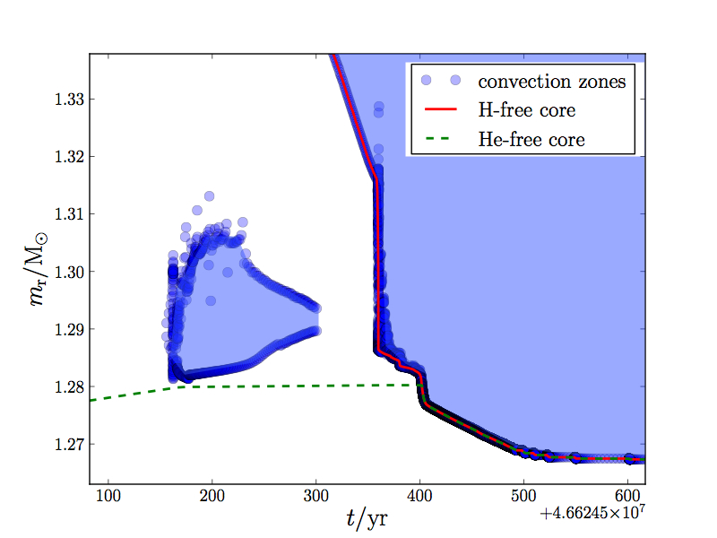
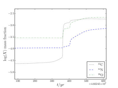
Figure 7.— Top panel: detail of the last phase of the second dredge-up of the $M_{\rm ZAMS}$=7$\,{\rm M}_{\odot}$ case; bottom panel: simultaneous surdace abundance evolution. After a so-called “dredge-out” phase the bottom of the core convection zone continues to penetrate (on Lagrangian coordinate) into the He-free core, bringing first ${}^{12}\mathrm{C}$ and then ${}^{16}\mathrm{O}$ into the envelope. The quantitative details of these mixing processes are sensitve to uncertain physics assumptions (see text). H- and He-free boundaries correspond to the mass coordinate where the mass fraction is respectively $\leq 10^{-4}$.

One may think that efficient hot-bottom burning in super-AGB stars, possibly boosted by the adoption of a higher value of $\alpha_{\mathrm{MLT}}$ could reduce even this additionally dredged-out O and C. Although individual third dredge-up events cannot be identified in the plot which shows the evolution of the envelope abundances, the $7\,{\rm M}_{\odot}$ sequence has been evolved through 18 thermal pulses with deep dredge-up. They cause the helium abundance to increase by $\Delta X(^{4}\mathrm{He})=0.0002$ per TP, which is the same as that found in the standard MLT sequence presented in Table 3. In order to reach a He mass-fraction abundance of $0.40$ another $105$ thermal pulse cycles would be needed, which is a very likely possibility considering the short interpulse periods and a reasonable range of possible mass-loss rates.

During the same initial 18 thermal pulses, the O abundance decreases by $0.16\,\mathrm{dex}$; consequently, over another $\sim 100$ TPs, a significant O depletion could be achieved. However, even if hot-bottom burning is able to further increase the abundance of He, and reduce the O abundance, by the desired amounts, the N abundance will become far too large. At the end of 18 thermal pulses, the ${}^{14}\mathrm{N}$ abundance has already increased by more than $2.3\,\mathrm{dex}$ and futher depletions of O will only add to the production of N. While the total CO enrichment in CO-core AGB stars can be controlled by fine-tuning the convection parameters, this is not obviously possible given the substantial enrichment of some super-AGB envelopes during the deep second dredge-up that reaches into the He-free core.

3.3.2 Initial mass dependence

The deep second dredge-up depends on assumptions of convective boundary mixing a well as on stellar mass. In order to determine the mass dependence of this mixing, as well as the upper and lower limiting masses for the super-AGB phases and the lifetimes for intermediate-mass AGB and super-AGB stars, we have calculated a fine grid of models with $4.0\leq M_{\rm ZAMS}/\,{\rm M}_{\odot}\leq 8.80$ with $\Delta M_{\rm ZAMS}=0.2\,{\rm M}_{\odot}$. Initial abundances are again according to the standard mix, and convective boundary mixing for H- and He-core burning with $f=0.014$ was included. At all other convective boundaries $f=0.010$ was assumed. For this grid v. 3372 of the MESA stellar evolution code was used, together with the NACRE (Angulo et al., 1999) reaction rates. From these calculations we find the lifetimes shown in Fig. 8.

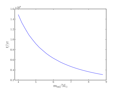
Figure 8.— Lifetimes of intermediate-mass AGB and super-AGB for the “standard” initial composition mix given in Table 1, determined from a grid of stellar models described in Sect. 3.3.2.

For $M_{\rm ZAMS}\geq 5.6\,{\rm M}_{\odot}$ with H-free core masses of $M_{\rm H}\geq 1.05\,{\rm M}_{\odot}$ the models show off-center C ignition, which in these models does not burn to completion in the central region in most cases. Deep second dredge-up that proceeds into the He-free core is found for $M_{\rm ZAMS}\geq 6.8\,{\rm M}_{\odot}$, and in these models the maximum He-free core mass before the reduction through the second dredge-up is $M_{\rm He}\geq 1.245\,{\rm M}_{\odot}$. Above this mass models predict large dredge-up of primary CNO as described in Sect. 3.3.1. For $M_{\rm ZAMS}\geq 7.6-7.8\,{\rm M}_{\odot}$ the core mass after the second dredge-up is at or just below the Chandraskhar mass, and more massive stars are expected to explode as supernova.

3.3.3 Convective boundary mixing effects

We have calculated another $7\,{\rm M}_{\odot}$ sequence without convective boundary mixing at the bottom of the convective envelope, but its behaviour with regard to the yields of He and CNO over the first dozen thermal pulses is very similar to the standard case. It shows the same deep second dredge-up. For these more massive super-AGB stars (cf. Sect. 3.3.2) the yields are dominated by the second dredge-up. The third dredge-up will only double the C+N+O abundance over the 18 computed thermal pulses (in the form of N), while the sequence without convective boundary mixing will not add additional CNO because there is no third dredge-up.

Table 3 Comparison of two thermal pulse cycles with standard ($\alpha_{\mathrm{MLT}}=1.73$) and increased mixing-length parameter ($\alpha_{\mathrm{MLT}}=2.40$): difference in H-shell interpulse and He-flash peak luminosities, dredge-up depth in $\,{\rm M}_{\odot}$ for second TP with deep dredge-up discussed in the text, surface He mass fraction increase over the two TP cycles as well as change of surface C, N and O over the two considered TP cycles.

	$\alpha_{\mathrm{MLT}}$=1.73	$\alpha_{\mathrm{MLT}}$=2.40
$\Delta\log L_{\rm H}[2.40-1.73]$	$\phantom{-}0.2$
$\Delta\log L_{\rm He}[2.40-1.73]$	$\phantom{-}0.3-0.5$
$\Delta m_{\mathrm{dup}}/\,{\rm M}_{\odot}$	$\phantom{-}7.1\times 10^{-4}$	$\phantom{-}1.66\times 10^{-3}$
$\Delta X(^{4}\mathrm{He})$	$\phantom{-}0.0004$	$\phantom{-}0.0023$
$\Delta\log X(C)$	$\phantom{-}0.28$	$\phantom{-}0.50$
$\Delta\log X(N)$	$\phantom{-}0.26$	$\phantom{-}0.50$
$\Delta\log X(O)$	$-0.10$	$-0.51$

Indeed, significant differences exist when convective boundary mixing is taken into account or when it is neglected altogether, in that the former is accompanied by effective third dredge-up with $\lambda\stackrel{{\scriptstyle<}}{{{}_{\sim}}}1$, while in the latter instance, the third dredge-up is absent. This has the important consequences that the cores of models with CBM do not grow, and they are therefore incapable of reaching the Chandrasekhar mass. As a result, they will become white dwarfs instead of evolving into ONeMg core-collapse supernova — unless they reside in a binary system, in which case they may still explode through an accretion-induced collapse (Fryer et al., 1999).

Another, potentially even more relevant consequence is the presence of $i$-process-conditions in super-AGB models with CBM (Herwig et al., 2012). Briefly, we find that dredge-up may – due to the short thermal time-scale at the core-envelope boundary – enter into the intershell immediately after the peak He-burning luminosity has been reached, and the He-intershell region is still convectively unstable. Then, depending on the convective mixing assumptions, protons may be convectively mixed into He-shell flash conditions, a situation in which high neutron densities of $N_{\mathrm{n}}\sim 10^{15}\mathrm{cm^{-3}}$ would be present (Cowan & Rose, 1977; Campbell et al., 2010; Herwig et al., 2011). The details of the $i$ process in super-AGB stars are still very uncertain, mostly due to our inability do correctly model the interaction between convective mixing and rapid, combustion-like burning of ${}^{12}\mathrm{C}$ + protons with the spherically symmetric assumption of stellar evolution, and 3D simulations, such as those in Herwig et al. (2011) will be required. However, within the present uncertainty Herwig et al. (2012) do consider a significant production of many n-capture elements in super-AGB stars from $i$ process, including La, a possibility. The implications of this possibilty will be discussed again later (Sect. 5.2).

3.3.4 Conclusion

Super-AGB stars with lower initial masses than $\sim 6.8\,{\rm M}_{\odot}$ and consequently lower He-free core masses ($<1.245\,{\rm M}_{\odot}$), would not suffer from the additional C and O envelope enrichment from deep second dredge-up. Stars in this mass range would in principle behave similar to the massive (CO core) AGB stars described in Sect. 3.2.1, and could have ejecta with the abundance pattern of the extreme distribution. The contribution of the most massive super-AGB stars must be minor due to the unavoidable and excessive O and N abundances that would characterize their ejecta. In order to identify the mass ranges and exact outcomes quantitatively in a more reliable way, the properties of convection in the deep stellar interior must be investigated in more detail.

In addition to the uncertainties in the treatment of convection, mass loss assumptions will significantly effect final and quantitative abundance predictions for ejecta (Ventura & D’Antona, 2011). In our models we have kept mass loss low in order to study the impact of convection uncertainties in isolation.

4. Summary and Discussion

In this section we provide a brief summary of our results, and then suggest a scenario for the formation of discrete populations of stars in $\omega$ Cen, with an emphasis on the bMS.

4.1. The main results of this investigation

Consistent with previous findings, we have found that the location of the bMS in the CMD of $\omega$ Cen can be reproduced by stellar models only if they assume significantly enhanced He abundances, in the range $Y=0.35-0.40$. Spectroscopic observations for giants in this system, and for one blue main-sequence star in NGC 2808, suggest that it is not only helium but also the CNO elements that have peculiar abundances, with mean values of [$m$/Fe] that have been described as the “extreme” Pop. II metals mixture (see Table 1). The bMS stars appear to have a higher iron content by about a factor of two than the dominant more metal-poor stellar population, which has [Fe/H] $\approx-1.7$.

The other, equally puzzling, CMD feature is the reddest MS that is commonly referred to as MS-a. We have shown that it is possible to match the photometry of these stars remarkably well using isochrones for the measured [Fe/H] value ($\approx-0.7$), provided that they also have rather high helium and CNO abundances. Indeed, it is possible that the bMS and MS-a populations differ only in terms of their iron abundances; i.e., that they are characterized by the same high values of $Y$ and the “extreme” [$m$/Fe] ratios. If this suggestion is correct, then all of the stellar populations in $\omega$ Cen would appear to have similar ages (within $\approx$ 1 Gyr given the chemical abundance uncertainties). For the MS-a stars to be significantly younger than, in particular, the most metal-deficient stars, the former would need to have much higher [CNO/Fe] abundances than those implied by the “extreme” mixture, since the latter abundances coupled with an old age (13 Gyr) are already needed to explain the very faint subgiant branch of the MS-a component.

We have further established, through simulations of AGB and super-AGB stars, that both of these types of stars, when forming out of the abundance mix which has been assumed for the first and dominant [Fe/H] $=-1.7$ population, are capable of ejecting winds with the high helium abundances that are needed to explain the CMD locations of the bMS stars. However, for the source of this material, we favour the massive AGB stars with CO cores and the less massive super-AGB stars with ONeMg cores. The wind ejecta of the most massive super-AGB stars with core masses $\geq 1.245\,{\rm M}_{\odot}$ are likely too enriched with N relative to He. In any case, even though either of the AGB models can eject matter with sufficiently high He abundances, it is not clear that they can produce ejecta with much larger He abundances than the upper limit that has been set from the CMD of the bMS ($Y\leq 0.4$). This imposes limits on the acceptable amount of dilution of the AGB material with gas that may still be present in the cluster or accreted from the intercluster medium in order to allow bMS stars to form with the indicated high He abundance pattern. Similarly, stellar populations with very low O abundances set tight constraints on the amount of allowable dilution (D’Ercole et al., 2011a).

The obvious question is then how to isolate the AGB ejecta from other gas that could be present; i.e., how to form the bMS stars out of just the ejecta from massive AGB stars instead of, for instance, the C-rich ejecta of somewhat lower-mass AGB stars (or possibly the Fe-rich ejecta of the more massive stars that explode as supernovae). The observationally established central concentration of stars with the “extreme” abundance mix (Johnson & Pilachowski, 2010) may very well be an important clue.

4.2. A scenario for the formation of multiple populations in globular clusters

We need to combine the stellar evolution results described thusfar with additional information in order to propose a general scenario for the formation of multiple populations, such as the bMS and MS-a/RG-a components of $\omega$ Cen. In particular, it is necessary to consider the early evolution of globular cluster progenitors in the gravitational potential of the host galaxy in combination with the cooling properties of AGB ejecta. To be sure, several aspects of this scenario have already been suggested and elaborated upon elsewhere, as pointed out below.

4.2.1 The progenitor of $\omega$ Cen and the orbit in the Galactic potential

The present-day orbit of $\omega$ Cen consists of a super-position of several oscillation components (Fig. 9), which suggests a complex capture mechanism that may very well have involved additional merging components. According to the backwards in time integrated orbit $\omega$ Cen has passed through the Galactic disk 13 times over the past $5\times 10^{8}$$\,\mathrm{yr}$ (Fig. 9), implying an average time interval between Galactic plane passage events of $\sim 40$ million years, with some variance. This estimate is approximate because of the uncertainty associated with the present-day velocity of $\omega$ Cen, and furthermore, the time interval may have shortened significantly since the capture of $\omega$ Cen’s progenitor, which may have been a dwarf galaxy (Bekki & Freeman, 2003; Böker, 2008; Marcolini & D’Ercole, 2008).

Figure 9.— The orbit of $\omega$Cen integrated assuming the present-day coordinates and positions given by Dinescu et al. (1999) and the Galaxy model described in Michel-Dansac et al. (2011). The orbit is computed by integrating backwards in time (i.e., after changing the sign of the present-day velocity) and shown for the past $500$ Myrs. The solar circle is indicated, at $R_{\odot}=8.5$ kpc, by a dotted line. Note that $\omega$Cen crosses the disk of the Galaxy roughly every $30$-$50$ Myrs.

In this primordial scenario of globular cluster formation (Padoan et al., 1997), $\omega$ Cen would have been much more massive (e.g., by a factor of $\sim 25$ according to Bekki & Freeman, 2003) when it was accreted, and it would have lost substantial fractions of its stellar and halo mass through tidal shocks at each pericentric passage. This process has been demonstrated through, for example, the $n$-body simulations by Peñarrubia et al. (2008) of dSph galaxies orbiting in the potential of galaxies like the Milky Way. These computations show that, depending on the orbital parameters (specifically the apocentric/pericentric ratio), within the first couple of pericentric passages (i) $\sim\,90\%$ of the dark matter halo is lost before any significant loss of stars occurs and (ii) mass is lost through outside-in “onion-peel” stripping. Through such tidal mass loss and evaporation episodes, it is quite conceivable that a much more massive progenitor would have ended up in $\omega$ Cen’s present state.

For globular clusters, Galactic plane passages have long been associated with the ram pressure stripping of the gas content of globular clusters (Tayler & Wood, 1975). We therefore assume that dark matter, stellar and gas components of the merging progenitor of $\omega$ Cen will be lost in varying proportions (as have, e.g. Valcarce & Catelan, 2011; D’Antona et al., 2011b), that will depend on the exact mass and orbit as well as the state of the Galaxy at the time of each interaction. The outcome would in any case be a complete purging of the gas in Galactic plane passages.

4.2.2 Supernova feedback and purging

Studies of supernova feedback in the context of the formation and evolution of galaxies show that star formation correlates with the mass of the galaxy and anti-correlates with the energy of the supernova (Scannapieco et al., 2008). Supernova feedback in low-mass systems leads to more severely limited and bursty star formation. If the progenitor of $\omega$ Cen had low enough mass in its early history, supernova feedback could have caused the purging of all of its gas. Indeed, an alternative to the Galactic plane passage purging is gas purging through supernova from stars with initial masses that bracket the AGB mass range (D’Ercole et al., 2008; Conroy & Spergel, 2011): stars more massive than super-AGB stars explode as type II supernovae, while those near the lower mass limit for massive AGB stars may lead to prompt (single-degenerate) supernovae of type Ia. In each of these cases, depending on the mass of the stellar system, SN explosions could purge the gas from it.

The cluster would, however, somehow need to be able to retain some of the iron from SN (Ia ?) explosions at later times in its evolution in order to enrich the gas out of which the relatively metal-rich MS-a population formed (Pancino et al., 2002; Origlia et al., 2003; Pancino et al., 2011). Similarly, at the epoch when stars were evolving into massive AGB stars, the potential well of $\omega$ Cen likely has to be deep enough for this system to retain the Fe ejecta from the small range of initial masses corresponding to the lowest mass type II SN, which have the lowest explosion energies. Most of the Fe that was produced by SN from more massive progenitors would have been blown out of the GC along with any intra-cluster gas.

D’Ercole et al. (2008) have pointed out that, if supernova from the electron-capture core collapses of the ONeMg cores of super-AGB stars have significantly lower explosion energies (Dessart et al., 2006), the (possibly) Fe-rich ejecta of those SN may be more easily retained by the cluster. This may be a viable alternative explanation of the small increase of the iron abundance in the bMS stars compared to the measured [Fe/H] of $\approx-1.7$ in the dominant initial stellar population. Marcolini et al. (2007) have investigated such aspects of the evolution of $\omega$ Cen through 3D hydrodynamic simulations of an isolated progenitor system that was assumed to be a dSph galaxy. They emphasized the differences between the SN II and Ia effects on the gas polution and the possibility of inhomogeneous enrichment of gas with SN Ia ejecta, but they admitted that tidal interactions with a host galaxy may have additional important consequences.

In any case, there are two, possibly complementary, processes available for the purging of all gas from the cluster — SN purging or periodic ram pressure/tidal shock purging through Galactic plane or pericentric passages. Which of these mechanisms dominates will depend on the detailed dynamical evolution of the system. In Sect. 4.2.4 we will explain why we favor the purging of gas via Galactic plane passages in the case of $\omega$ Cen because of the unique effects that this process can potentially have on the star formation and chemical evolution histories of such a system.

4.2.3 The Cooling of the Gas Ejected by AGB Stars

Cooling flows from AGB ejecta have been investigated by D’Ercole et al. (2008), on the assumption of a cooling function for the solar metallicity by Rosen & Bregman (1995). However, the ejecta of the first generation AGB stars have a much lower metallicity, and therefore one would expect that the cooling of this material would be much less efficient. Since the cooling flow of AGB ejecta to the center of a system like $\omega$ Cen is an important ingredient in most scenarios (ours, and those by, e.g., D’Ercole et al., 2008; D’Antona et al., 2011a; Bekki, 2011) for the origin of the He-rich second generation (see Sect. 4.2.4), it is worthwhile to examine the cooling properties of a gas having the “extreme” metals mixture, and how it differs in comparison with that predicted for for “standard” (i.e., typical) Pop. II abundances.

While the actual abundances in the $\omega$ Cen bMS stars may be somewhat milder than in our “extreme” abundance mix, those abundances out of which the stars formed may have been subject to some limited amount of dilution (cf. Sect. 4.1). Any assumption of dilution requires the AGB ejecta to be more extreme than the bMS stars in $\omega$ Cen. What exactly the abundance of the cooling flow is will depend on when the dilution takes place, something that is difficult to know. In any case, it is appropriate to consider the cooling properties of material with“extreme” composition as representative of what the AGB ejecta may look like.

Figure 10.— The radiative cooling coefficient for a gas having the indicated chemical abundances (also see the text). The loci with filled circles superimposed represent the sum of the contributions to $\Lambda/(n_{e}n{\rm H})$ from H, He, C, N, O, and Ne, as well as free-free emission (which dominates at $\log T\mathrel{\hbox{\raise 2.58334pt\hbox{$>$}\kern-7.3194pt\lower 2.15277pt\hbox{$\sim$}}}5.8$). For a sake of clarity, only a few of the contributions to the total cooling curves from individual elements have been plotted.

In the limit where the photoionization caused by the stellar radiation field can be neglected; i.e., when collisional ionization conditions apply, the radiative cooling coefficient (in erg cm${}^{-3}\,$s^-1) varies as a function of $\log\,T$ approximately as shown in Fig 10 for three different heavy-element mixtures. This plot was generated using the computer code developed by VandenBerg (1978) to model the outflows of gas from present-day globular clusters to try to explain why the gas that is ejected into the interstellar medium (ISM) through normal (low-velocity) mass-loss processes is not observed. (When these systems pass through the Galactic disk, any gas that might have collected is expected to be swept out by the ram pressure exerted by the local ISM, but gas should accumulate to detectable levels over the rest of their orbits in at least the most massive systems.) If photoionization is unimportant, then the ionization state of the gas can be determined simply from the condition that the number of collisional ionizations per unit time for any ion is exactly equal to rate of electron recombinations, which is independent of the density. Once the ionization state has been calculated, the radiative energy losses due to free-free and free-bound transitions, and from the transitions to lower energy levels from high-excitation states that were populated by recombination or inelastic electron collisions, can be determined (see the VandenBerg paper for a detailed description of the relevant physics).

Since the energy loss rates due to recombination radiation and collision-induced line emission are proportional to $n_{e}n_{Z,z}$, where $n_{e}$ is the electron density and $n_{Z,z}$ is the number density of atoms having an atomic number $Z$ and an ionic charge $z$, the radiative cooling coefficient $\Lambda/(n_{e}n_{\rm H})$ can be derived for any mixture once the fractional ionization, $n_{Z,z}/n_{Z}$, has been calculated and the abundances of each element are specified relative to hydrogen (i.e., $n_{Z}/n_{\rm H}$). The solid curves in Fig. 10 assume the solar metal abundances given by Asplund et al. (2009), while the dot-dashed and dashed curves give, in turn, the temperature dependence of $\Lambda/(n_{e}n_{\rm H})$ for an Asplund et al. (2009) mixture having [$m$/H] $=0.4$ for all of the $\alpha$-elements (“standard” composition in Table 1) and then scaled to [Fe/H] $=-1.4$ and for the “extreme” mix from Table 1 scaled to [Fe/H] $=-1.4$. In these latter cases, the adopted mass fractions of helium correspond to $Y=0.25$ and $Y=0.38$, respectively. (Since these results may be of some use to future investigations that take into account the cooling of the gas, the total cooling coefficients, as represented by the loci with filled circles attached to them, have been listed as a function of $\log\,T$ in Table 4.)

Table 4Radiative Cooling Coefficient: $\log\,(\Lambda/n_{e}n_{\rm H}$)

	[Fe/H] $=0.0$	[Fe/H] $=-1.4$
$\log T$		Standard Mix	Extreme Mix
3.80	-24.694	-24.694	-24.694
3.85	-24.626	-24.626	-24.626
3.90	-24.425	-24.425	-24.425
3.95	-24.012	-24.013	-24.013
4.00	-23.489	-23.490	-23.490
4.05	-22.972	-22.973	-22.973
4.10	-22.513	-22.514	-22.514
4.15	-22.162	-22.163	-22.163
4.20	-21.992	-21.994	-21.993
4.25	-22.005	-22.009	-22.009
4.30	-22.110	-22.121	-22.118
4.35	-22.228	-22.257	-22.248
4.40	-22.319	-22.386	-22.360
4.45	-22.359	-22.493	-22.433
4.50	-22.353	-22.589	-22.482
4.55	-22.308	-22.679	-22.514
4.60	-22.232	-22.752	-22.509
4.65	-22.134	-22.783	-22.453
4.70	-22.022	-22.736	-22.337
4.75	-21.896	-22.589	-22.168
4.80	-21.761	-22.377	-21.968
4.85	-21.631	-22.183	-21.788
4.90	-21.530	-22.079	-21.682
4.95	-21.466	-22.076	-21.651
5.00	-21.443	-22.130	-21.653
5.05	-21.469	-22.202	-21.654
5.10	-21.493	-22.266	-21.644
5.15	-21.482	-22.308	-21.629
5.20	-21.454	-22.328	-21.632
5.25	-21.429	-22.338	-21.713
5.30	-21.415	-22.342	-21.912
5.35	-21.402	-22.343	-22.161
5.40	-21.412	-22.362	-22.381
5.45	-21.496	-22.443	-22.559
5.50	-21.680	-22.602	-22.712
5.55	-21.889	-22.771	-22.836
5.60	-22.046	-22.892	-22.931
5.65	-22.140	-22.968	-23.002
5.70	-22.205	-23.022	-23.060
5.75	-22.298	-23.089	-23.120
5.80	-22.467	-23.190	-23.187
5.85	-22.677	-23.293	-23.244
5.90	-22.857	-23.363	-23.275
5.95	-22.974	-23.402	-23.280
6.00	-23.031	-23.419	-23.266
6.05	-23.050	-23.423	-23.242
6.10	-23.046	-23.417	-23.215
6.15	-23.028	-23.405	-23.190
6.20	-23.001	-23.388	-23.175
6.25	-22.972	-23.368	-23.173
6.30	-22.947	-23.348	-23.183

For the sake of clarity, just a few of the contributions to the total cooling rates, due to the individual metals, are shown. Nitrogen is of particular interest in view of the wide range in its abundance in the three mixtures, and it is quite evident that the cooling due to this element in the “extreme” [Fe/H] $=-1.4$ mixture is much greater than that predicted for the other two cases (including, in particular, solar abundances). It is also much greater, by factors of $\mathrel{\hbox{\raise 2.58334pt\hbox{$>$}\kern-7.3194pt\lower 2.15277pt\hbox{$\sim$}}}60$, than the contributions due to C and O because the latter are much less abundant. As helium is mainly responsible for the bump in the radiative cooling coefficient at $\log\,T\approx 4.9$, the effects of increasing $Y$ from 0.25, in the “normal” mix, to 0.38, in the “extreme” mix, are clearly significant. The main point of Fig. 10 is that a gas with high N and He abundances will cool much more efficiently than a gas having a more normal mix of metals and a helium abundance that is closer to the primordial value. Indeed, the total radiative cooling coefficient for the former approaches that for a gas having solar abundances (at least at $\log T\mathrel{\hbox{\raise 2.58334pt\hbox{$<$}\kern-7.74998pt\lower 2.15277pt\hbox{$\sim$}}}5.3$).

The presence of an intense stellar radiation field, such as that produced by extremely hot ($\sim 50,000$ K) $uv$-bright stars, would heat the gas and ionize many of the atoms and ions that are responsible for radiative cooling, and thereby hinder or prevent the infall of gas towards the cluster center. However, such stars, which represent a much more significant source of heating than large populations of blue HB stars (see VandenBerg 1978), are quite rare ($\mathrel{\hbox{\raise 2.58334pt\hbox{$<$}\kern-7.74998pt\lower 2.15277pt\hbox{$\sim$}}}1$ star is expected in present-day GCs at any given time although this number is expected to have been larger in the past). Consequently, it is difficult to describe the interplay between the radiation field and the material shed by AGB stars, without performing detailed simulations of globular clusters when they were younger and much more massive than they are now.

It will be interesting to see what impact these more realistic cooling properties will have on simulations that include the cooling flow of AGB stars (as well as that of primordial matter, e.g. D’Ercole et al., 2008). Considering the “extreme” abundance mix as an upper limit of the boost in cooling efficiency over the “standard” mix, the cooling efficiency of realistic AGB ejecta are smaller by a factor $\stackrel{{\scriptstyle>}}{{{}_{\sim}}}4$ compared to solar cooling curves employd be those simulations. In any case, we do assume in the following that AGB ejecta will cool and accumulate in the cluster center (see also Bekki, 2011, who comes to the same conclusion).

4.2.4 A possible scenario

The lifetime of the $7$ and $5\,{\rm M}_{\odot}$ stellar evolutionary models is $4.6$ and $9.1\times 10^{7}\,\mathrm{yr}$, respectively (Fig. 8). The similarity of the time interval between successive Galactic plane passages of $\omega$ Cen and the time it would take super-AGB and massive AGB stars to expel their He- and N-enriched and O-depleted wind ejecta could very well conspire in such a way that, by the time that the massive- and super-AGB stars are about to eject their envelopes, the wind material from more massive stars has been entirely, or mostly, cleared out of the system and the AGB winds are released into an empty, or nearly empty, cluster. Stars with an extreme abundance mix would subsequently form, but the star formation process would be terminated when the remaining gas is cleared out during the next passage through the plane. This would isolate the AGB yields and enable formation out of pure AGB ejecta.

The scenario for the origin of multiple populations starts with the progenitor evolution of $\omega$ Cen. The proto-cluster, possibly a dwarf galaxy (Sect. 4.2.1), would have a fully populated initial-mass function (IMF) when it merges with the Galaxy. Star formation may have going on at a low level since its formation, corresponding to the low-metallicity tail below the dominant (first) generation at [Fe/H]$\sim-1.7$ in $\omega$ Cen. But somehow, we assume that the dominant stellar content of the $\omega$ Cen progenitor would be the first generation, and it would have been produced by a star formation burst, maybe triggered by the tidal interactions associated with the complex capture processes indicated by the present-day orbit (Fig. 9, Sect. 4.2.1; see also Bekki & Freeman, 2003). Assuming that $\omega$ Cen is then in an orbit fairly similar to the one shown in Fig. 9, the first Galactic plane passage gas purging could occur $\mathrel{\hbox{\raise 2.58334pt\hbox{$<$}\kern-7.74998pt\lower 2.15277pt\hbox{$\sim$}}}40$ million years later. This would remove all of the remnant gas ejecta from stars more massive than super-AGB stars.

Over the next $50$–$90$ million years, until the next Galactic plane passage, AGB stars and possibly super-AGB stars would eject winds into the empty cluster, with abundance patterns that have helium and oxygen abundances that closely resemble those attributed to the bMS stars in $\omega$ Cen (Sect. 3). These ejecta would initially have the same spatial distribution througout the cluster as the AGB donor stars, but radiative cooling processes would cause the gas to sink preferentially towards the center of the cluster, as disccussed in Sect. 4.2.3.

According to Bekki (2011), the accumulation of gas and the subsequent formation of the second generation of stars will be fully under way after $\sim 3$ million years, and be largely completed in the central core within $\mathrel{\hbox{\raise 2.58334pt\hbox{$<$}\kern-7.74998pt\lower 2.15277pt\hbox{$\sim$}}}13$ million years. This leaves enough time until the next Galactic plane passage to fully populate a second-generation IMF.

Bekki suggests that the second-generation IMF may be bottom heavy in order to explain the high ratio of second- to first-generation stars. However, as mentioned in Sect. 4.2.1 and noted by Bekki, among others, further mass is lost from the system through subsequent pericentric passages from the outside-in (see the discussion in Sect. 4.2.1). In fact, the fraction of first generation stars that has to be lost (from the outside-in) in order to match the observed bMS star fraction can be easily estimated for a given mass range of intermediate mass stars that release their winds between Galactic plane passages. This mass range will of course depend on the (not accurately known) orbital parameters of $\omega$ Cen at that time. Based on the calculated model grid described in Sect. 3.3.2 we adopt a lower limit for this mass range as $M_{\mathrm{min}}=4$ – $5\,{\rm M}_{\odot}$ by the requirement to produce large He and N enhancements, and $M_{\mathrm{max}}=6.8$ – $7.7\,{\rm M}_{\odot}$ taking into account possibly prohibitive dredge-out (Sect. 3.3.1) and excluding the high-mass regime of core-collapse supernova. With this mass range assumptions the IMF of Kroupa (2001) implies that intermediate mass stars will eject $5.2\pm 2.0\%$ of the mass of the first generation stars (assuming $20\%$ of the initial stellar mass will end up in the white dwarf). The number of bMS stars has been projected to be $24$ – $35\%$ of the first generation stars (Bedin et al., 2004; Sollima et al., 2007b). These numbers imply that in order to account for the observed fraction of bMS stars $78.3\pm 8.3$ – $85.1\pm 5.7\%$ of first generation stars must have been lost from the outside (assuming a normal IMF). This seems to be reasonable in our scenario (cf. Sect. 4.2.1), considering also that the central location of the bMS population implies that it contributes only marginally to the mass that is lost from the cluster through dynamical interactions. We therefore assume that the second generation IMF is normal.

Then, the second generation will also include massive stars. The associated supernova will explode in the very center of the still relatively massive cluster, which is the most favorable location for the retention of SN ejecta (Marcolini et al., 2007). Depending on when these SN occur with respect to the timing of the second Galactic plane passage, the ejecta from the most massive second-generation supernova may be lost during the passage through the disk, but afterwards, it seems plausible that Fe-rich ejecta from the lowest-mass SNe could be retained in the core region. Further down the IMF, super-AGB stars and possibly the most massive AGB stars with CO core could again contribute to what would be the third generation. This would again form in the cluster core before the third Galactic plane passage would terminate this last major star formation episode. This third generation would have a substantially higher iron abundance from second-generation SN, compared to that of the bMS, and it would have enhanced He and CNO. Furthermore, this third generation, which may be the RGB-a/MS-a population discussed in Sect. 2, would consist of significantly fewer stars than the second generation. As before, this star formation event would end when the cluster makes its fourth passage through the Galactic plane and the remaining gas is purged. After that diminishing numbers would make it impossible to discern further populations in the cluster core.

Star formation would not be impossible in other parts of the cluster after this fourth Galactic plane passage, but it is possible that, by this time, the mass of the cluster has decreased to the extent that it is no longer possible to retain the ejecta from supernovae. In this case, the total cluster wind ejecta may now, $\geq 2\times 10^{8}\,\mathrm{yr}$ after the initial star formation burst, be dominated by the increasing number of intermediate-mass ($\sim 3-4\,{\rm M}_{\odot}$) first-generation stars that are ending their lives. The ejecta would again be $s$-process rich, but also C-rich. Stars forming out of these “late” wind ejecta would have rather low [Fe/H] since they are formed out of first (and possibly second) generation star ejecta. This may explain why the $s$-process enhanced stars do not show the same central concentration compared with the He-enriched stars, and why the $s$-process enhancements seem to be increasing already at relatively low [Fe/H], not much higher than that of the first generation. As a matter of fact, the data of Marino et al. (2012, Fig. 6 & 7) indeed shows two La-enrichment sequences, one belonging to what is identified as the ’first generation’ that correlates with C, and one that correlates rather with N, and associated with the second generation. In our scenario, the C-rich, low [Fe/H] and high La-abundance stars would in fact be the fourth generation (see Sect. 5.2 for more discussion on this point).

As discussed in Sect. 4.2.2, some workers (e.g. D’Ercole et al., 2008; Conroy & Spergel, 2011) favour the idea that the purging of gas from clusters is mostly due to supernova. Massive-star SN II explosions would clear out the gas until a lower mass limit is reached where either SN IIs no longer occur, or the explosions are so weak that they are incapable of removing all of the gas. Whether or not SN are effective in purging the gas sufficiently to enable the formation of a second generation out of the isolated ejecta of stars from a particular mass range will not only depend on the total mass of the system and the energy of the supernova, but also on their location within the cluster (progenitor). While SN purging clearly seems to be a viable mechanism in some (possibly less massive) clusters, our proposed scenario appears to be capable of explaining the detailed properties of the very unusual case of $\omega$ Cen, such as the small difference in [Fe/H] between the first and second stellar generations, and the larger difference in metallicity between the second and third generations. Moreover, it should also work for other clusters that are massive enough to retain SN ejecta.

Table 5 Summary of the four generations identified in the Galactic plane passage gas purging model for $\omega$ Cen, and how they match with the cluster analysis of Gratton et al. (2011) and with the observational properties reported in DOrazi:2011jf and Marino et al. (2012) (see text for details, in particular Sect. 5.3).

generation	parent generation	expected abundance markers	Gratton et al. (2011) group	corresponds to features reported in Marino et al. (2012)	Leiden star numbers D’Orazi et al. (2011)
first	proto-cluster	low Fe; normal He, La; high $\alpha$, high (from r-process) Eu	#4, #6		16015, 37247, 33011,
second, bMS	first	low O, intermediate Fe; high He, N, Na, n-capture	#3, #2a	low O, high Na (most extreme?) for medium [Fe/H]	41039, 46092, 34029
third, MS-a/RGB-a	second	high Fe, C+N+O; higher N, He, n-capture	#2b	highest Na & La for highest [Fe/H]	60066, 60073, 34180, 48323, 54022
fourth	first (second)	low (medium) Fe; normal He, medium O, Na, high C, n-capture	#5, #1	O, Na, N, C - La relation of O-poor/Na-rich group	44462

5. Conclusions

5.1. Implications of the Galactic plane passage gas purging model

As D’Ercole et al. (2008) put it, He-rich populations (like the bMS in $\omega$ Cen) are only the tip of the iceberg of the phenomenon of second (or third, etc.) stellar populations. While our scenario of periodic gas purging events caused by the passages of clusters through the Galactic plane appears to be able to explain quite naturally the origin of the helium-rich bMS in $\omega$ Cen (and possibly the more Fe-rich MS-a/RGB-a population, as well), one can readily imagine that this simple picture, if applied to clusters having a wide range of progenitor histories (e.g., masses and orbits), may, in fact, generate quite a variety of realizations in the globular clusters that we observe today. Since each population would be associated with the ejecta arising from stars within one, or very few, relatively narrow initial mass ranges, isolated by successive Galactic plane passages that clear out any gas that had accumulated since the last passage, any two (or more) populations that are present in different clusters should not be identical, though possibly similar. The contributing segments of the IMF are statistically selected according to the progenitor orbit and the merger history.

However, in our scenario, Galactic plane passage intervals of $40$ to $100$ million years do favor the formation of a second, helium-rich population. If the delay is $40$ million years (as also found by Marino et al., 2012), upper and lower mass limits can both be imposed by the Galactic plane passages. For time intervals as large as $100$ million years, only the lower mass cut-off for the progenitor stars of the second generation is set by the Galactic plane passage, while the higher mass cut-off would be due to SN purging. In fact, this case is similar to the model suggested by D’Ercole et al. (2008, Sect. 3.1), who adopt $100$ Myr for their parameter $\Delta t_{\mathrm{f}}$. They do not mention what sets this time interval, aside from noting that, if $\Delta t_{\mathrm{f}}$ was longer, SN Ia and C-producing AGB stars would contribute to the second-generation star formation (see the above discussion). This is indeed why $\Delta t_{\mathrm{f}}$ should not be longer if the desired outcome is a helium-rich second generation, but we suggest that the main reason is that the Galactic plane passages which clear out the gas and terminate star formation occur every $\mathrel{\hbox{\raise 2.58334pt\hbox{$<$}\kern-7.74998pt\lower 2.15277pt\hbox{$\sim$}}}100$ Myr.

In summary, the simple principle of periodic Galactic plane passage purging in combination with low-velocity winds from massive AGB stars AGB wind predictions and their preferential cooling properties, may be able to account for the bMS abundances including its central concentration, the MS-a/RGB-a abundance patterns as well as the homogeneous distribution of and wide range of [Fe/H] observed in s-enhanced stars.

5.2. O-Na anti-correlation, n-capture element abundances, and other observed properties of $\omega$ Cen

One of the (possibly defining, Carretta et al., 2010) features of globular clusters is the more or less complete presence of the O-Na anticorrelation. How does it fit in with the Galactic plane passage gas purging model? The key question is whether (a) the anti-correlation occurs within a sub-population, or (b) it is the superposition of the rather distinct O-Na abundances of the present sub-populations. The answer will depend on how the latter are identified. If one uses only the [Fe/H] abundance (e.g. D’Antona et al., 2011b) one may indeed combine N-rich/C-poor with C-rich/N-poor stars into one group (Marino et al., 2012, Fig. 2) and conclude that abundance anti-correlations are present even within a sub-population.

This view point may motivate, or even require as an explanationof the Na-O anti-correlation, a dilution scenario (D’Ercole et al., 2011b) which assumes that, while second-generation stars form in the cluster, unprocessed pristine gas is accreted from outside of the cluster. However, if option (b) is in fact the case, for example, if the sub-population identification purely by [Fe/H] is not entirely accurate, then an alternative interpretation of the anti-correlation is possible in which dilution may not play an important role.

Option (b) may also be favoured by observations of rather uniform Al abundances in the SGB-a population (in our scenario the third generation, see Table 5) by Pancino et al. (2011), suggesting that no anti-correlation is present in this sub-population. Although we have tried to resist the temptation in this paper to apply the Galactic plane passage gas purging model to other clusters we note that Carretta et al. (2012) found that the anti-correlations involving Al, Mg, Na and O in NGC 6752 – another GC for which multiple populations possibly including large He-enrichements have been found – manifest themselves in a rather discrete fashion, in which different levels of enhancement and depletion cluster around discrete values that can be associated with individual sub-populations, rather than a continuous distribution that would be sugggested by a pure dilution mechanism.

The Galactic plane passage gas purging scenario implies that two distinct populations may have the same [Fe/H] abundance, and therefore that a collection of stars with the same [Fe/H] may not necessarily belong to the same population. As a matter of fact, many possible elemental markers if used by themselves may lead to degenerate grouping of stars. In order to identify those stars that most likely represent a coevally formed sub-population, several elemental markers should be combined. Such a “group” analysis, taking into account four abundance features simultaneously, has been performed by Gratton et al. (2011). The resultant sub-population identification is indeed rather suggestive of option (b) mentioned in the previous paragraph (superposition of the distinct O-Na abundance markers from sub-population). Of course, there is always a concern that the particular choice of group-finding criteria biases the process. For that reason the sub-population identification by Gratton et al. (2011) may be evolve in the future when more observational data are added to this kind of analysis. In any case, this approach seems to be an improvement over just using [Fe/H] to identify sub-populations. As a consequence, we have no compelling need for the dilution mechanism in our model for $\omega$ Cen.

Our scenario has a few more implications – some of which are summarized in Table 5 – that we would like to briefly discuss. It offers an alternative interpretation of the star formation time-scale determination of D’Antona et al. (2011b) that was based on the assumption that Fe in the MS-a/RGB-a populations originates in SN Ia. In our scenario, Fe for the third generation (MS-a/RGB-a) comes from the lowest mass, second generation SN II after the second Galactic plane passage (Sect. 4.2.4), which would be in agreement with the $\alpha$-element abundance patterns found by Gratton et al. (2011) for the most Fe-rich population labeled #2b. The time-scale limit from SN Ia would therefore not apply. In addition, star formation can take place even after the formation of this third generation from the late stellar winds of low-mass first-generation stars.

In fact, if we retain our chemical evolution time range determination from CMD considerations ($\mathrel{\hbox{\raise 2.58334pt\hbox{$<$}\kern-7.74998pt\lower 2.15277pt\hbox{$\sim$}}}1$ Gyr, Sect. 2), stars in the fourth generation can form from the slow wind ejecta of first-generation stars down to $1.8\,{\rm M}_{\odot}$. For stars with $\stackrel{{\scriptstyle<}}{{{}_{\sim}}}2.6\,{\rm M}_{\odot}$ these ejecta would be C-rich (as well as La-rich from the main $s$ process). Because the first-generation donor stars are not centrally concentrated, the fourth generation stars that form out of them would also not be centrally located — if the cooling efficiency of lower-mass AGB ejecta are smaller, or because the mass of the cluster is already smaller at this point. Indeed, Johnson & Pilachowski (2010) report no radial gradient for [La/Fe]. In any case, the observations reported by Marino et al. (2012) show that there are two different La-enrichment sequences, one associated with increasing C (O-rich/Na-poor group) and one associated with low O and high Na. In our scenario the former represents the transition from first to fourth generation, while the latter is associated with both the second and, possibly for even more extreme levels of enrichment, the third generation.

If we interprete the correlation of C with La in the O-rich/Na-poor group of Marino et al. (2012) as the result of the third dredge-up in $1.8$ – $2.6\,{\rm M}_{\odot}$ first (and maybe second slightly higher [Fe/H]) generation stars, then their Fig. 7 implies that O and Na could also be the result of the third dredge-up. In fact, the slight increase of O with [Fe/H] in the O-rich/Na-poor group has been perceived to be quite a puzzle that implies an extra source of O. However, the models of Herwig (2004b, Fig. 6) for $\mathrm{[Fe/H]}=-2.3$ do indeed predict $\mathrm{[C/Fe]}=3.0$, $\mathrm{[O/Fe]}=1.8$ and $\mathrm{[Na/Fe]}=1.3$ for the average abundance in ejecta of a $2\,{\rm M}_{\odot}$ model. The O comes from the dredge-up of primary He-burning products that becomes appreciable at these low metal abundances, and such O enhancements are indeed observed in many CEMP stars that may carry the mass transfer signature from genuine low-metallicity AGB stars (for example, Sivarani et al., 2006; Kennedy et al., 2011). The Na in the $2\,{\rm M}_{\odot}$ model comes from $s$ process in the He-shell flash convection zone, where the neutron from the ${}^{22}\mathrm{Ne}(\alpha,\mathrm{n})^{25}\mathrm{Mg}$ reaction is captured again by ${}^{22}\mathrm{Ne}$. The predicted enrichment levels suggest that a population which forms out of such ejecta should have about twice the enrichment of C compared to O and Na, which seems to be consistent with the Marino et al. (2012) data.

Star Leiden  44462 has been tentatively identified by D’Orazi et al. (2011) as a mass transfer object in order to account for the extremely high C abundance. Although radial velocity measurements may support this possibility, an alternative interpretation is that this star is part of the fourth generation (Table 5) which forms out of the slow winds of $1.8$ – $2.6\,{\rm M}_{\odot}$ first (or second for higher [Fe/H]) generation stars. In fact, this star coincides very well with the C-La correlation sequence shown in Marino et al. (2012, Fig.  7, upper right panel).

But the O-poor/Na-rich group of Marino et al. (2012), as well as all but the lowest [Fe/H] stars in D’Orazi et al. (2011), also show marked n-capture enhancements. Since in these stars the C abundance is low, the heavy elements cannot come from these lower-mass AGB stars. Instead we have to consider higher-mass AGB stars as well as super-AGB stars. The n-capture element predictions of Karakas et al. (2012), e.g. their $6\,{\rm M}_{\odot}$, $Z=0.0001$ stellar evolution model, are based mostly on the ${}^{22}\mathrm{Ne}$ neutron source in the He-shell flash convection zone (although some contribution from a ${}^{13}\mathrm{C}$-pocket may be present as well). Clearly, the $s$-process models for these low-metallicity intermediate-mass stars are quantiatively still rather uncertain (cf. Sect. 3.2.2). However, the models of Karakas et al. (2012) do predict that higher mass AGB stars at this metal content do produce $s$-process elements, possibly with significant enrichment factors, and with a ratio of light (ls: Sr, Y, Zr, Rb) to heavy (hs: Ba, La) $s$-process-elements that is higher than in the ejecta of lower mass stars. Such a signature would qualitatively agree with the n-capture abundances reported for the N-rich, intermediate- (bMS, second generation) and high- (MS-a/RGB-a, third generation) Fe group by (D’Orazi et al., 2011).

In addition to the n-capture production by ${}^{22}\mathrm{Ne}(\alpha,\mathrm{n})^{25}\mathrm{Mg}$ in the He-intershell in intermediate mass AGB stars, we mentioned in Sect. 3.3.2 the possible presence of $i$-process-conditions in super-AGB models with CBM (Herwig et al., 2012), which would provide for another “non-standard” source of n-capture elements in stars that produce He-rich and O-poor populations in $\omega$ Cen. Both of these sources would be responsible for the La-enhanced sequence of the O-poor/Na-rich group reported by Marino et al. (2012).

An important consequence of this discussion is the notion that the Na enhancements which we expect from AGB stars from $1.8\,{\rm M}_{\odot}$ all the way up to the super-AGB stars at $\stackrel{{\scriptstyle<}}{{{}_{\sim}}}6.8$ – $7.7\,{\rm M}_{\odot}$ may always be expected to go along with n-capture element enhancements. This assessment is supported by the La-Na correlations of both the O-rich/Na-poor and the O-poor/Na-rich group of Marino et al. (2012, lower-right panel of Fig. 7).

5.3. Summary

Obviously the observational identification of the four generations that we have specified – within the Galactic plane passage gas purging model – as the result of highly idealized processes, is complicated by interference and superposition effects as well as contributions from, e.g., supernova purging, turbulent and tidal mixing, and cooling and mass loss flows, all of which are expected in a real cluster. In addition, observational uncertainties may cause some migration between observationally identified groups, which is in addition to the principal difficulty of deciding on the criteria and procedures that are used to group stars (as discussed at the beginning of Sect. 5.2). These complications impose a limit to the accuracy that we can expect in how well observed properties can be matched to the predictions of any scenario. The best that we can ask for at this point is rather qualitative agreement, and with this goal in mind we have summarized the alignment of the Galactic plane passage gas purging model with some recently reported observational properties of $\omega$ Cen in Table 5.

While most of the entries in Table 5 are based on our discussion in the previous sections there is a noteworthy peculiarity in the most metal-poor group (“first” generation) which should represent the genuine first generation stars. In Sect. 5.2 we made the case that the observational data may support the case of the superposition of separate sub-populations forming the overall anti-correlation in $\omega$ Cen. It seems that, in fact, in this lowest [Fe/H] bin there are signs of an intrinisic anti-correlation with at most an unclear signature of n-capture enhancement. Groups #6 and #4 of Gratton et al. (2011) taken together display a significant scatter in the [Na/O] ratio, while the lowest-metallicity bin of D’Orazi et al. (2011) includes two very N-rich stars (see also Marino et al., 2012). This possible substructure in the most metal-poor population in $\omega$ Cen cannot be explained by the Galcatic plane passage gas purging model, and may be a relic of the proto-cluster object.

References

- Anderson (1997) Anderson, A. J. 1997, PhD thesis, UNIVERSITY OF CALIFORNIA, BERKELEY
- Anderson et al. (2008) Anderson, J., Sarajedini, A., Bedin, L. R., et al. 2008, AJ, 135, 2055
- Angulo et al. (1999) Angulo, C., Arnould, M., & Rayet, M. et al. 1999, Nucl. Phys., A 656, 3, NACRE compilation
- Asplund et al. (2009) Asplund, M., Grevesse, N., Sauval, A. J., & Scott, P. 2009, ARA&A, 47, 481
- Bedin et al. (2005) Bedin, L. R., Cassisi, S., Castelli, F., Piotto, G., Anderson, J., Salaris, M., Momany, Y., & Pietrinferni, A. 2005, MNRAS, 357, 1038
- Bedin et al. (2004) Bedin, L. R., Piotto, G., Anderson, J., Cassisi, S., King, I. R., Momany, Y., & Carraro, G. 2004, ApJ, 605, L125
- Bekki (2011) Bekki, K. 2011, MNRAS, 412, 2241
- Bekki & Freeman (2003) Bekki, K. & Freeman, K. C. 2003, MNRAS, 346, L11
- Bellazzini et al. (2004) Bellazzini, M., Ferraro, F. R., Sollima, A., Pancino, E., & Origlia, L. 2004, A&A, 424, 199
- Bellini et al. (2010) Bellini, A., Bedin, L. R., Piotto, G., Milone, A. P., Marino, A. F., & Villanova, S. 2010, AJ, 140, 631
- Bellini et al. (2009) Bellini, A., Piotto, G., Bedin, L. R., King, I. R., Anderson, J., Milone, A. P., & Momany, Y. 2009, A&A, 507, 1393
- Blöcker (1995) Blöcker, T. 1995, A&A, 297, 727
- Böker (2008) Böker, T. 2008, ApJ, 672, L111
- Bragaglia et al. (2010) Bragaglia, A., Carretta, E., Gratton, R. G., Lucatello, S., Milone, A., Piotto, G., D’Orazi, V., Cassisi, S., Sneden, C., & Bedin, L. R. 2010, ApJ, 720, L41
- Brown & Wallerstein (1993) Brown, J. A. & Wallerstein, G. 1993, AJ, 106, 133
- Busso et al. (2007) Busso, G., Cassisi, S., Piotto, G. et al. 2007, A&A, 474, 105
- Calamida et al. (2009) Calamida, A., Bono, G., Stetson, P. B.et al. 2009, ApJ, 706, 1277
- Campbell et al. (2010) Campbell, S. W., Lugaro, M., & Karakas, A. I. 2010, A&A, 522, L6
- Carretta et al. (2012) Carretta, E., Bragaglia, A., Gratton, R. G., Lucatello, S., & D’Orazi, V. 2012, ApJ, 750, L14
- Carretta et al. (2010) Carretta, E., Bragaglia, A., Gratton, R. G., Recio-Blanco, A., Lucatello, S., D’Orazi, V., & Cassisi, S. 2010, A&A, 516, A55
- Cassisi et al. (2009) Cassisi, S., Salaris, M., Anderson, J., Piotto, G., Pietrinferni, A., Milone, A., Bellini, A., & Bedin, L. R. 2009, ApJ, 702, 1530
- Cassisi et al. (2008) Cassisi, S., Salaris, M., Pietrinferni, A., Piotto, G., Milone, A. P., Bedin, L. R., & Anderson, J. 2008, ApJ, 672, L115
- Cayrel et al. (2004) Cayrel, R., Depagne, E., Spite, M. et al. 2004, A&A, 416, 1117
- Conroy & Spergel (2011) Conroy, C. & Spergel, D. N. 2011, ApJ, 726, 36
- Cowan & Rose (1977) Cowan, J. J. & Rose, W. K. 1977, ApJ, 212, 149
- Cox & Giuli (1968) Cox, J. P. & Giuli, R. T. 1968, Principles of stellar structure (New York, Gordon and Breach [1968])
- D’Antona & Caloi (2008) D’Antona, F. & Caloi, V. 2008, MNRAS, 390, 693
- D’Antona et al. (2011a) D’Antona, F., D’Ercole, A., Marino, A. F., Milone, A. P., Ventura, P., & Vesperini, E. 2011a, ApJ, 736, 5
- D’Antona et al. (2011b) —. 2011b, ApJ, 736, 5
- Decressin et al. (2007) Decressin, T., Meynet, G., Charbonnel, C., Prantzos, N., & Ekström, S. 2007, A&A, 464, 1029
- Denissenkov & VandenBerg (2003) Denissenkov, P. A. & VandenBerg, D. A. 2003, ApJ, 593, 509
- D’Ercole et al. (2011a) D’Ercole, A., D’Antona, F., & Vesperini, E. 2011a, MNRAS, 415, 1304
- D’Ercole et al. (2011b) —. 2011b, MNRAS, 415, 1304
- D’Ercole et al. (2008) D’Ercole, A., Vesperini, E., D’Antona, F., McMillan, S. L. W., & Recchi, S. 2008, MNRAS, 391, 825
- Dessart et al. (2006) Dessart, L., Burrows, A., & Ott, C. 2006, ApJ, 644, 1063
- Dinescu et al. (1999) Dinescu, D. I., van Altena, W. F., Girard, T. M., & López, C. E. 1999, AJ, 117, 277
- D’Orazi et al. (2011) D’Orazi, V., Gratton, R. G., Pancino, E., Bragaglia, A., Carretta, E., Lucatello, S., & Sneden, C. 2011, A&A, 534, A29
- Ferguson et al. (2005) Ferguson, J. W., Alexander, D. R., Allard, F., Barman, T., Bodnarik, J. G., Hauschildt, P. H., Heffner-Wong, A., & Tamanai, A. 2005, ApJ, 623, 585
- Ferraro et al. (2004) Ferraro, F. R., Sollima, A., Pancino, E., Bellazzini, M., Straniero, O., Origlia, L., & Cool, A. M. 2004, ApJ, 603, L81
- Freytag et al. (1996) Freytag, B., Ludwig, H.-G., & Steffen, M. 1996, A&A, 313, 497
- Fryer et al. (1999) Fryer, C., Benz, W., Herant, M., & Colgate, S. A. 1999, ApJ, 516, 892
- García-Berro & Iben (1994) García-Berro, E. & Iben, Jr., I. 1994, ApJ, 434, 306
- Gratton et al. (2011) Gratton, R. G., Johnson, C. I., Lucatello, S., D’Orazi, V., & Pilachowski, C. 2011, A&A, 534, A72
- Gratton et al. (2000) Gratton, R. G., Sneden, C., Carretta, E., & Bragaglia, A. 2000, A&A, 354, 169
- Gustafsson et al. (2008) Gustafsson, B., Edvardsson, B., Eriksson, K., Jørgensen, U. G., Nordlund, Å., & Plez, B. 2008, A&A, 486, 951
- Herwig (2000) Herwig, F. 2000, A&A, 360, 952
- Herwig (2004a) —. 2004a, ApJ, 605, 425
- Herwig (2004b) —.. 2004b, ApJS, 155, 651
- Herwig (2005) —.. 2005, ARAA, 43, 435
- Herwig et al. (1997) Herwig, F., Blöcker, T., Schönberner, D., & El Eid, M. F. 1997, A&A, 324, L81
- Herwig et al. (2012) Herwig, F., Jones, S., Pignatari, M., Paxton, B., & VandenBerg, D. 2012, ApJ, ”in preparation”
- Herwig et al. (2011) Herwig, F., Pignatari, M., Woodward, P. R., Porter, D. H., Rockefeller, G., Fryer, C. L., Bennett, M., & Hirschi, R. 2011, ApJ, 727, 89
- Hilker et al. (2004) Hilker, M., Kayser, A., Richtler, T., & Willemsen, P. 2004, A&A, 422, L9
- Hughes & Wallerstein (2000) Hughes, J. & Wallerstein, G. 2000, AJ, 119, 1225
- Iben et al. (1997) Iben, Jr., I., Ritossa, C., & Garcia-Berro, E. 1997, ApJ, 489, 772
- Iglesias & Rogers (1996) Iglesias, C. A. & Rogers, F. J. 1996, ApJ, 464, 943
- Johnson & Pilachowski (2010) Johnson, C. I. & Pilachowski, C. A. 2010, ApJ, 722, 1373
- Johnson et al. (2008) Johnson, C. I., Pilachowski, C. A., Simmerer, J., & Schwenk, D. 2008, ApJ, 681, 1505
- Karakas et al. (2012) Karakas, A. I., García-Hernández, D. A., & Lugaro, M. 2012, ApJ, 751, 8
- Kayser et al. (2006) Kayser, A., Hilker, M., Richtler, T., & Willemsen, P. G. 2006, A&A, 458, 777
- Kennedy et al. (2011) Kennedy, C. R., Sivarani, T., Beers, T. C., Lee, Y. S., Placco, V. M., Rossi, S., Christlieb, N., Herwig, F., & Plez, B. 2011, AJ, 141, 102
- King et al. (2012) King, I. R., Bedin, L. R., Cassisi, S., Milone, A. P., Bellini, A., Piotto, G., Anderson, J., Pietrinferni, A., & Cordier, D. 2012, AJ, 144, 5
- Kroupa (2001) Kroupa, P. 2001, MNRAS, 322, 231
- Lee et al. (1999) Lee, Y.-W., Joo, J.-M., Sohn, Y.-J., Rey, S.-C., Lee, H.-C., & Walker, A. R. 1999, Nature, 402, 55
- Lub (2002) Lub, J. 2002, in ASP Conf. Series, Vol. 265, Omega Centauri, A Unique Window into Astrophysics, ed. F. van Leeuwen, J. D. Hughes, & G. Piotto, 95
- Ludwig et al. (1999) Ludwig, H., Freytag, B., & Steffen, M. 1999, A&A, 346, 111
- Marcolini & D’Ercole (2008) Marcolini, A. & D’Ercole, A. 2008, Proc. IAU, 4, 152
- Marcolini et al. (2007) Marcolini, a., Sollima, A., D’Ercole, A., Gibson, B. K., & Ferraro, F. R. 2007, MNRAS, 382, 443
- Marino et al. (2012) Marino, A. F., Milone, A. P., Piotto, G. et al. 2012, ApJ, 746, 14
- Marino et al. (2011) Marino, A. F., Milone, A. P., Piotto, G., Villanova, S., Gratton, R., D’Antona, F., Anderson, J., Bedin, L. R., Bellini, A., Cassisi, S., Geisler, D., Renzini, A., & Zoccali, M. 2011, ApJ, 731, 64
- McCall (2004) McCall, M. L. 2004, AJ, 128, 2144
- McSaveney et al. (2007) McSaveney, J. A., Wood, P. R., Scholz, M., Lattanzio, J. C., & Hinkle, K. H. 2007, MNRAS, 378, 1089
- Michel-Dansac et al. (2011) Michel-Dansac, L., Abadi, M. G., Navarro, J. F., & Steinmetz, M. 2011, MNRAS, 414, L1
- Milone et al. (2012) Milone, A. P., Piotto, G., Bedin, L. R. et al. 2012, ApJ, 744, 58
- Norris (2004) Norris, J. E. 2004, ApJ, 612, L25
- Origlia et al. (2003) Origlia, L., Ferraro, F. R., Bellazzini, M., & Pancino, E. 2003, ApJ, 591, 916
- Padoan et al. (1997) Padoan, P., Jimenez, R., & Jones, B. 1997, MNRAS, 285, 711
- Pancino et al. (2000) Pancino, E., Ferraro, F. R., Bellazzini, M., Piotto, G., & Zoccali, M. 2000, ApJ, 534, L83
- Pancino et al. (2011) Pancino, E., Mucciarelli, A., Bonifacio, P., Monaco, L., & Sbordone, L. 2011, A&A, 534, A53
- Pancino et al. (2002) Pancino, E., Pasquini, L., Hill, V., Ferraro, F. R., & Bellazzini, M. 2002, ApJ, 568, L101
- Paxton et al. (2011) Paxton, B., Bildsten, L., Dotter, A., Herwig, F., Lesaffre, P., & Timmes, F. 2011, ApJS, 192, 3
- Peñarrubia et al. (2008) Peñarrubia, J., Navarro, J. F., & McConnachie, A. W. 2008, ApJ, 673, 226
- Piotto et al. (2007) Piotto, G., Bedin, L. R., Anderson, J. et al. 2007, ApJ, 661, L53
- Piotto et al. (2005) Piotto, G., Villanova, S., Bedin, L. R. et al. 2005, ApJ, 621, 777
- Porter & Woodward (2000) Porter, D. H. & Woodward, P. R. 2000, ApJS, 127, 159
- Proffitt & Michaud (1991) Proffitt, C. R. & Michaud, G. 1991, ApJ, 380, 238
- Rey et al. (2004) Rey, S.-C., Lee, Y.-W., Ree, C. H., Joo, J.-M., Sohn, Y.-J., & Walker, A. R. 2004, AJ, 127, 958
- Ritossa et al. (1999) Ritossa, C., García-Berro, E., & Iben, I. J. 1999, ApJ, 515, 381
- Robinson et al. (2004) Robinson, F. J., Demarque, P., Li, L. H. et al. 2004, MNRAS, 347, 1208
- Romano et al. (2007) Romano, D., Matteucci, F., Tosi, M. et al. 2007, MNRAS, 376, 405
- Rosen & Bregman (1995) Rosen, A. & Bregman, J. N. 1995, ApJ, 440, 634
- Sbordone et al. (2011) Sbordone, L., Salaris, M., Weiss, A., & Cassisi, S. 2011, A&A, 534, A9
- Scannapieco et al. (2008) Scannapieco, C., Tissera, P. B., White, S. D. M., & Springel, V. 2008, MNRAS, 389, 13
- Schlegel et al. (1998) Schlegel, D. J., Finkbeiner, D. P., & Davis, M. 1998, ApJ, 500, 525
- Siess (2007) Siess, L. 2007, A&A, 476, 893
- Siess (2010) —. 2010, A&A, 512, A10+
- Sirianni et al. (2005) Sirianni, M., Jee, M. J., Benítez, N. et al. 2005, PASP, 117, 1049
- Sivarani et al. (2006) Sivarani, T., Beers, T. C., Bonifacio, P. et al. 2006, A&A, 459, 125
- Smith et al. (2000) Smith, V. V., Suntzeff, N. B., Cunha, K., Gallino, R., Busso, M., Lambert, D. L., & Straniero, O. 2000, AJ, 119, 1239
- Sollima et al. (2007a) Sollima, A., Ferraro, F. R., & Bellazzini, M. 2007a, MNRAS, 381, 1575
- Sollima et al. (2007b) Sollima, A., Ferraro, F. R., Bellazzini, M., Origlia, L., Straniero, O., & Pancino, E. 2007b, ApJ, 654, 915
- Sollima et al. (2005a) Sollima, A., Ferraro, F. R., Pancino, E., & Bellazzini, M. 2005a, MNRAS, 357, 265
- Sollima et al. (2005b) Sollima, A., Pancino, E., Ferraro, F. R., Bellazzini, M., Straniero, O., & Pasquini, L. 2005b, ApJ, 634, 332
- Stanford et al. (2006) Stanford, L. M., Da Costa, G. S., Norris, J. E., & Cannon, R. D. 2006, ApJ, 647, 1075
- Stanford et al. (2007) —. 2007, ApJ, 667, 911
- Suntzeff & Kraft (1996) Suntzeff, N. B. & Kraft, R. P. 1996, AJ, 111, 1913
- Tayler & Wood (1975) Tayler, R. & Wood, P. 1975, MNRAS, 171, 467
- Valcarce & Catelan (2011) Valcarce, A. A. R. & Catelan, M. 2011, A&A, 533, A120
- van Loon et al. (2007) van Loon, J. T., van Leeuwen, F., Smalley, B., Smith, A. W., Lyons, N. A., McDonald, I., & Boyer, M. L. 2007, MNRAS, 382, 1353
- VandenBerg et al. (2012) VandenBerg, D. A., Bergbusch, P. A., Dotter, A. et al. 2012, ArXiv e-prints
- VandenBerg et al. (2006) VandenBerg, D. A., Bergbusch, P. A., & Dowler, P. D. 2006, ApJS, 162, 375
- VandenBerg et al. (2010) VandenBerg, D. A., Casagrande, L., & Stetson, P. B. 2010, AJ, 140, 1020
- VandenBerg et al. (2000) VandenBerg, D. A., Swenson, F. J., Rogers, F. J., Iglesias, C. A., & Alexander, D. R. 2000, ApJ, 532, 430
- Ventura & D’Antona (2009) Ventura, P. & D’Antona, F. 2009, A&A, 499, 835
- Ventura & D’Antona (2011) —. 2011, MNRAS, 410, 2760
- Villanova et al. (2007) Villanova, S., Piotto, G., King, I. R. et al. 2007, ApJ, 663, 296