A dynamical condition for differentiability of Mather’s average action

Abstract

We prove the differentiability of $\beta$ of Mather function on all homology classes corresponding to rotation vectors of measures whose supports are contained in a Lipschitz Lagrangian absorbing graph, invariant by Tonelli Hamiltonians. We also show the relationship between local differentiability of $\beta$ and local integrability of the Hamiltonian flow.

1 Introduction

Given a Tonneli Lagrangian $L$, Mather introduced the $\beta$-function of $L$, which is a convex and superlinear function. Many interesting properties of the Euler–Lagrange flow can be derived from the study of the behaviour of the $\beta$-function. Understanding whether or not this function is differentiable and what are the implications of its re-gularity to the dynamics of the system is an interesting problem. This type of problem was developed by D. Massart in several works as, for example, [14] and [15].

Even in this context, D. Massart and A. Sorrentino get in the work Differentiability of Mather’s average action and integrability on closed surfaces (see [16]) the relation, on closed surfaces, between the differentiability of $\beta$-function and the integrability of the system. However there are examples of systems which are not integrable but have invariant Lipschitz Lagrangian graphs, i.e. invariant graphs of the form $\mathcal{G}_{\eta,u}=graph\left(\eta+du\right)$ where $\eta$ is a closed one-form and $u$ is a function of class $C^{1}$ with Lipschitz differential.

Motivated by these problems, in this work we study the differentiability of $\beta$ at homologies $h$ whose the measures with vector rotation $h$ are supported on an invariant Lipschitz Lagrangian graph. We obtain differentiability of $\beta$ in these homologies if the invariant graph is an absorbing graph, i.e. a graph which not contain $\omega$-limit of minimizing curves out of it. More precisely, we prove the following theorem:

Theorem 1

Let $\mathcal{G}_{\eta,u}$ be an invariant Lipschitz Lagrangian graph. Then $\mathcal{G}_{\eta,u}$ is absor-bing if and only if $\beta$ is differentiable at $h$ for all $h\in\partial\alpha\left(\left[\eta\right]\right)$ and $\mathcal{A}_{\left[\eta\right]}^{\ast}=\mathcal{G}_{\eta,u}.$

One can derive some consequences of this result. For instance, if the system is locally Lipschitz integrable on an invariant Lipschitz Lagrangian graph $\mathcal{G}_{\eta,u}\subset T^{\ast}M,$ i.e. there exists a neighborhood $\mathcal{V}$ of $\mathcal{G}_{\eta,u}$ in $T^{\ast}M$ foliated by disjoint invariant Lipschitz Lagrangian graphs, of course that the graphs contained in $\mathcal{V}$ are absorbing, so the following result is a local version of a result of D. Massart and A. Sorrentino (See [16], Lemma 5).

Theorem 2

Let $\mathcal{G}_{\eta,u}$ be an invariant Lipschitz Lagrangian graph. If $H$ is locally Lipschitz integrable on $\mathcal{G}_{\eta,u}$, then there exists a neighborhood $U_{0}\subset H^{1}\left(M;\mathbb{R}\right)$ of $\left[\eta\right]$ such that $\beta$ is differentiable at any point of $V=\bigcup\nolimits_{c\in U_{0}}\partial\alpha\left(c\right).$

We prove the converse of Theorem 2 in the case $M$ equals torus $\mathbb{T}^{2}$ (see Theorem 15). In this case, the set $V=\bigcup\nolimits_{c\in U_{0}}\partial\alpha\left(c\right),$ obtained in the above statement, is open in $H_{1}\left(\mathbb{T}^{2};\mathbb{R}\right)$. Then we geralize ([16], Theorem 3) to local case.

We also give a particular attention to existence of neighborhood contained in the tiered Mañé, introduced by M-C. Arnaud in [1], and its relation with the local integrability of system and therefore with the local differentiability of $\beta.$ Indeed, we prove a local version of a result of M-C. Arnaud (See [2], Theorem 1), in the Section 5, Corollary 13.

2 Preliminaries

Let $M$ be a compact connected manifold and $TM$ its tangent bundle. A Tonelli’s Lagrangian is a function $L:TM\rightarrow\mathbb{R}$ of class at least $C^{2}$ which is convex and superlinear. Let us recall the main concepts introduced by Mather in [17]. Let $\mathcal{M}\left(L\right)$ be the set of probabilities on the Borel $\sigma$-algebra on $TM$ which are invariant under the Euler–Lagrange flow $\varphi_{t}^{L}$. The Euler Lagrange flow generated by $L$ does not change by adding a closed one form $\eta$ and the action of a probability measure $\mu\in\mathcal{M}\left(L\right)$, defined by

$$A_{L-c}\left(\mu\right)=\int_{TM}\left(L-\eta\right)d\mu$$

depends only on the cohomology class $c=[\eta]\in H^{1}(M;{\mathbb{R}})$.

The minimal action value, which also depends only on the cohomology class $c=[\eta],$ is denoted by $-\alpha(c),$ that is:

$$\alpha(c)=-\inf_{\mu\in\mathcal{M}\left(L\right)}A_{L-c}\left(\mu\right).$$

Mather proved that the function $c\mapsto\alpha\left(c\right),$ so-called $\alpha$ of Mather function, is convex and superlinear. It is known that $\alpha(c)$ is the energy level that contains the Mather set for the cohomology class $c$:

$${\widetilde{\mathcal{M}}}_{c}=\overline{\bigcup_{\mu}\operatorname{supp}(\mu)},$$

where the union is taken over the set of Borel probability measures $\mu\in\mathcal{M}\left(L\right)$ called $c$-minimizing, i.e. $\alpha(c)=-A_{L-c}\left(\mu\right).$ The set ${\widetilde{\mathcal{M}}}_{c}$ is a compact invariant set which is a graph over a compact subset $\mathcal{M}_{c}$ of $M$, the projected Mather set (see [17]). $\mathcal{M}_{c}$ is laminated by curves, which are global (or time independent) minimizers.

Given a probability measure $\mu\in\mathcal{M}\left(L\right)$, its homology or its rotation vector is defined as the unique $\rho\left(\mu\right)\in H_{1}(M;{\mathbb{R}})$ such that

$$\left\langle\rho(\mu),\left[\omega\right]\right\rangle=\int_{TM}\omega d\mu,$$

for all closed 1-forms $\omega$ on $M.$ By convexity, we can consider the dual Fenchel of $\alpha$, called $\beta$ of Mather function, as

$$\beta\left(h\right)=\inf_{\rho(\mu)=h}A_{L}\left(\mu\right).$$

Mather also proved that the $\beta$ function is convex and superlinear. We say that a measure $\mu\in\mathcal{M}\left(L\right)$ with $\rho\left(\mu\right)=h$ is $h$-minimizing if $\beta\left(h\right)=A_{L}\left(\mu\right).$ The set $\widetilde{\mathcal{M}}^{h}$ is the union of supports of probability measures $h$-minimizing.

In general, the maps $\alpha$ and $\beta$ are neither strictly convex, nor differentiable. The projection on domain of regions of graph where either map is affine are called flats. Actually, if the map is strictly convex at a point, the flat is this only point and if the map is not strictly convex, the flat is non-trivial. By duality we have the inequality

$$\alpha(c)+\beta\left(h\right)\geq\left\langle c,h\right\rangle,\forall c\in H^{1}(M;{\mathbb{R}}),\forall h\in H_{1}(M;{\mathbb{R}}),$$

called Fenchel inequality. Given $c\in H^{1}(M;{\mathbb{R}})$ (resp. $h\in H_{1}(M;{\mathbb{R}})$), the homology class $h\in H_{1}(M;{\mathbb{R}})$ (resp. $c\in H^{1}(M;{\mathbb{R}})$) achieving equality in the Fenchel inequality is called subderivative of $\alpha$ in $c$ (resp. subderivative of $\beta$ in $h$). The set composed by subderivatives of $\alpha$ in $c$ (resp. subderivatives of $\beta$ in $h$) is called Legendre transform of $c$ (resp. $h$), and denoted $\partial\alpha\left(c\right)$ (resp. $\partial\beta\left(h\right)$). Therefore, $\partial\alpha\left(c\right)$ is a flat of $\beta$ and $\partial\beta\left(h\right)$ is a flat of $\alpha.$ By convexity, the sets $\partial\alpha\left(c\right)$ and $\partial\beta\left(h\right)$ are non-empty.

Many interesting properties of the Euler–Lagrange flow can be derived from the study of the behaviour of the $\beta$-function. For instance, if $h$ is an extremal point of $\beta$-function, i.e. $h$ is not convex combination of two elements in a same flat of $\beta,$ then there exist ergodic measures with homology $h$ (see [13]).

Let us recall that we can associate to such a Tonelli’s Lagrangian $L$ the Hamiltonian function $H:T^{\ast}M\rightarrow\mathbb{R}$ via Legendre transform $\mathcal{L}:TM\rightarrow T^{\ast}M,$ which under our assumption, is a diffeomorphism of class at least $C^{1}$, defined in coordinates by

$$\mathcal{L}\left(x,v\right)=\left(x,\frac{\partial L}{\partial v}\left(x,v\right)\right).$$

Actually, $H$ is the dual Fenchel of $L$ and also is convex and superlinear. Given a cohomology class $c$ and a closed 1-form $\eta_{c}$ with $\left[\eta_{c}\right]=c,$ we consider the Hamilton-Jacobi equation

$$H\left(x,\eta_{c}\left(x\right)+d_{x}u\right)=\alpha(c).$$ (HJ)

A Lipschitz function $u:M\rightarrow\mathbb{R}$ is called a subsolution of Hamilton-Jacobi for the Lagrangian $L-c$ if for some closed 1-form $\eta_{c}$ with $\left[\eta_{c}\right]=c,$ we have

$$H\left(x,\eta_{c}\left(x\right)+d_{x}u\right)\leq\alpha(c),$$ (1)

at almost every point. Note that this definition is equivalent to the notion of viscosity subsolutions (see [9]). We denote by $C^{1,1}$ the set of differentiable functions with Lipschitz differential. Observe that a $C^{1,1}$ function $u$ is solution of (HJ) if and only if the graph of $\eta_{c}+du,$ denoted by $\mathcal{G}_{\eta_{c},u},$ is invariant under Hamiltonian flow.

We now recall the definition of calibrated curves (see [9]). If $u:M\rightarrow\mathbb{R}$ is a subsolution of Hamilton-Jacobi for $L-c$, we say that the curve $\gamma:I\rightarrow M$ is $\left(u,L-c,\alpha\left(c\right)\right)$-calibrated if, for the representative $\eta_{c}$ of the cohomology class $c$ given in $\left(\ref{fo5}\right)$, we have the equality

$$u\left(\gamma\left(t\right)\right)-u\left(\gamma\left(t^{\prime}\right)\right)=\int\nolimits_{t^{\prime}}^{t}L\left(\gamma\left(s\right),\dot{\gamma}\left(s\right)\right)-\eta_{c}\left(\dot{\gamma}\left(s\right)\right)+\alpha\left(c\right)ds,$$

for all $t^{\prime},t\in I.$ The subset $\widetilde{\mathcal{I}}_{c}(u)$ of $TM$ is defined by

$$\widetilde{\mathcal{I}}_{c}(u)=\left\{\left(x,v\right)\in TM:\gamma_{\left(x,v\right)}\text{ is }\left(u,L-c,\alpha\left(c\right)\right)\text{-calibrated}\right\},$$

where $\gamma_{\left(x,v\right)}=\pi\circ\varphi_{t}^{L}\left(x,v\right)$. The set $\widetilde{\mathcal{I}}_{c}(u)$ is invariant and the curves contained in it are called curves $c$-minimizing.

Using the sets $\widetilde{\mathcal{I}}_{c}(u)$, one can give (see [10]) the following characterization of the Mañé set and of the Aubry set:

$$\widetilde{\mathcal{N}}_{c}=\bigcup\limits_{u\in SS_{c}}\widetilde{\mathcal{I}}_{c}\left(u\right)\text{ and }\widetilde{\mathcal{A}}_{c}=\bigcap\limits_{u\in SS_{c}}\widetilde{\mathcal{I}}_{c}\left(u\right),$$

where $SS_{c}$ is the set of subsolution of (HJ) for $L-c$. These invariant sets contain the Mather set and have interesting dynamical properties, for instance $\widetilde{\mathcal{A}}_{c}$ also is graph whose projection is laminated by global minimizers and it is chain recurrent. The Mañé set $\widetilde{\mathcal{N}}_{c}$ is connected and chain transitive (see for instance [7]).

Using the duality between Lagrangian and Hamiltonian, via Legendre transform, we define the sets of Mather, Aubry and Mañé in the cotangent bundle, respectively by

$$\mathcal{M}_{c}^{\ast}=\mathcal{L}\left(\widetilde{\mathcal{M}}_{c}\right),\mathcal{A}_{c}^{\ast}=\mathcal{L}\left(\widetilde{\mathcal{A}}_{c}\right)\text{ e }\mathcal{N}_{c}^{\ast}=\mathcal{L}\left(\widetilde{\mathcal{N}}_{c}\right).$$

One useful way to produce invariant Lipschitz Lagrangian graphs is to show that $\pi\left(\mathcal{A}_{c}^{\ast}\right)=M.$ If this is the case, the Theorem 2.5 of [10] says that there exists an unique solution $u$ of (HJ) for the Lagrangian $L-c$ which is $C^{1,1}$ and such that $\mathcal{A}_{c}^{\ast}$ is the graph of $\eta_{c}+du,$ for some $\eta_{c}$ representative of cohomology class $c.$

3 Absorbing sets

If $u:M\rightarrow\mathbb{R}$ is a subsolution of (HJ) for $L-c$, we denote by $\widetilde{\mathcal{I}}_{c}^{+}\left(u\right)$ the subset of $TM$ defined as

$$\widetilde{\mathcal{I}}_{c}^{+}\left(u\right)=\left\{\left(x,v\right):\gamma_{\left(x,v\right)}|_{\left[0,+\infty\right)}\text{ is }\left(u,L-c,\alpha\left(c\right)\right)\text{-calibrated}\right\},$$

where $\gamma_{\left(x,v\right)}$ is the curve defined on $\mathbb{R}$ by

$$\gamma_{\left(x,v\right)}\left(t\right)=\pi\circ\varphi_{t}^{L}\left(x,v\right).$$

The forward Mañe set is defined by

$$\widetilde{\mathcal{N}}_{c}^{+}=\bigcup\limits_{u\in SS_{c}}\widetilde{\mathcal{I}}_{c}^{+}\left(u\right),$$

where $SS_{c}$ is the set of critical subsolutions for the Lagrangian $L-c.$ We define the forward tiered Mañé set as the union of all forward Mañe sets, i.e. the subset of $TM$ given by

$$\mathcal{N}_{+}^{T}\left(L\right)=\bigcup\limits_{c\in H^{1}\left(M\right)}\widetilde{\mathcal{N}}_{c}^{+}.$$

Definition 3

We say that an invariant set $\Lambda\subset TM$ is an absorbing set if for all $\left(x,v\right)\in\mathcal{N}_{+}^{T}\left(L\right)$ we have

$$\omega\left(x,v\right)\subset\Lambda\Rightarrow\left(x,v\right)\in\Lambda$$

Definition 4

Let $\mathcal{G\subset}T^{\ast}M$ be an invariant Lipschitz Lagrangian graph. We say that $\mathcal{G}$ is an absorbing graph if $\mathcal{L}^{-1}\left(\mathcal{G}\right)$ is an absorbing set.

Lemma 5

If $\left(x,v\right)\in\widetilde{\mathcal{N}}_{c}^{+},$ then the $\omega$-limit set $\omega\left(x,v\right)$ is contained in $\widetilde{\mathcal{A}}_{c}.$

Proof: In fact, let $\left(x,v\right)\in\widetilde{\mathcal{N}}_{c}^{+}$ and $\gamma:\mathbb{R}\rightarrow M\$the projection of Euler-Lagrange solution $\gamma\left(t\right)=\pi\circ\varphi_{t}^{L}\left(x,v\right)$ curve such that $\gamma|_{\left[0,+\infty\right)}$ is $\left(\overline{u},L-c,\alpha\left(c\right)\right)$-calibrated for some $\overline{u}\in$ $SS_{c}.$ This means that there exists a closed 1-form $\eta_{c}$ with $\left[\eta_{c}\right]=c$ such that $H\left(x,\eta_{c}\left(x\right)+d_{x}\overline{u}\right)\leq\alpha\left(c\right)$ at almost every point and

$$\overline{u}\left(\gamma\left(t\right)\right)-\overline{u}\left(\gamma\left(t^{\prime}\right)\right)=A_{L-\eta_{c}+\alpha\left(c\right)}\left(\gamma|_{\left[t^{\prime},t\right]}\right)\text{ for all }0<t^{\prime}<t.$$

Let $\left(y,z\right)\in\omega\left(x,v\right),$ i.e. $\left(y,z\right)=\lim_{n\rightarrow\infty}\left(\gamma,\dot{\gamma}\right)\left(t_{n}\right)$ with $t_{n}\rightarrow\infty.$

Let us consider $\sigma:\mathbb{R}\rightarrow M\$the projection of the Euler-Lagrange solution $\sigma\left(t\right)=\pi\circ\varphi_{t}^{L}\left(y,z\right).$ Given a Hamilton-Jacobi subsolution $u:M\rightarrow\mathbb{R}$ belonging to $SS_{c}$, there exists a closed 1-form $\xi_{c}$ with $\left[\xi_{c}\right]=c$ and $H\left(x,\xi_{c}\left(x\right)+d_{x}u\right)\leq\alpha\left(c\right)$ at almost every point. It follows from ([9], Proposition 4.2.3) that $u$ satisfies

$$u\left(\gamma\left(t\right)\right)-u\left(\gamma\left(t^{\prime}\right)\right)\leq A_{L-\xi_{c}+\alpha\left(c\right)}\left(\gamma|_{\left[t^{\prime},t\right]}\right),\forall t^{\prime}<t.$$

We can consider $V$ a $C^{\infty}\left(M\right)$ function such that $\eta_{c}=\xi_{c}+dV.$ Thus, if $s>0$ and $\left(t_{k}\right)$ and $\left(t_{m}\right)$ are two subsequences of $\left(t_{n}\right)$ such that $t_{k}-s>t_{m}+s$ and $t_{k},t_{m}>s,$ we have

$$A_{L-\xi_{c}+\alpha\left(c\right)}\left(\sigma|_{\left[-s,s\right]}\right)+u\left(\sigma\left(-s\right)\right)-u\left(\sigma\left(s\right)\right)$$

$$=\lim_{m,k}\left[A_{L-\xi_{c}+\alpha\left(c\right)}\left(\gamma|_{\left[t_{m}-s,t_{m}+s\right]}\right)+u\left(\gamma\left(t_{k}-s\right)\right)-u\left(\gamma\left(t_{m}+s\right)\right)\right]$$

$$\leq\lim_{m,k}\left[A_{L-\xi_{c}+\alpha\left(c\right)}\left(\gamma|_{\left[t_{m}-s,t_{m}+s\right]}\right)+A_{L-\xi_{c}+\alpha\left(c\right)}\left(\gamma|_{\left[t_{m}+s,t_{k}-s\right]}\right)\right]$$

$$=\lim_{m,k}A_{L-\xi_{c}+\alpha\left(c\right)}\left(\gamma|_{\left[t_{m}-s,t_{k}-s\right]}\right)$$

$$=\lim_{m,k}\left[A_{L-\xi_{c}-dV+\alpha\left(c\right)}\left(\gamma|_{\left[t_{m}-s,t_{k}-s\right]}\right)+V\left(\gamma\left(t_{k}-s\right)\right)-V\left(\gamma\left(t_{m}-s\right)\right)\right]$$

$$=\lim_{m,k}A_{L-\eta_{c}+\alpha\left(c\right)}\left(\gamma|_{\left[t_{m}-s,t_{k}-s\right]}\right)+V\left(\gamma\left(-s\right)\right)-V\left(\gamma\left(-s\right)\right)$$

$$=\lim_{m,k}\overline{u}\left(\gamma\left(t_{k}-s\right)\right)-\overline{u}\left(\gamma\left(t_{m}-s\right)\right)$$

$$=\overline{u}\left(\gamma\left(-s\right)\right)-\overline{u}\left(\gamma\left(-s\right)\right)=0.$$

Therefore

$$A_{L-\xi_{c}+\alpha\left(c\right)}\left(\sigma|_{\left[-s,s\right]}\right)\leq u\left(\sigma\left(s\right)\right)-u\left(\sigma\left(-s\right)\right).$$

The opposite inequality holds because $u$ is a Hamilton-Jacobi subsolution (see [9], Proposition 4.2.3). This shows that

$$\left(y,z\right)\in\bigcap\limits_{u\in SS_{c}}\widetilde{\mathcal{I}}_{c}\left(u\right)=\widetilde{\mathcal{A}}_{c}.$$

 

Examples of absorbing graphs are the so-called Schwartzman strictly ergodic graphs (see [11]), i.e. invariant graphs $\Lambda$ which support an invariant measure with full support. In fact, let $\mu$ the invariant measure supported in $\Lambda$ with $\rho\left(\mu\right)=h.$ If $\omega\left(x,p\right)\subset\Lambda$ for some $\left(x,p\right)\in\mathcal{L}\left(\widetilde{\mathcal{I}}_{c}^{+}\left(L\right)\right),$ then it follows from above lemma that $\omega\left(x,p\right)\subset\mathcal{A}_{c}^{\ast}\cap\Lambda.$ In particular,

$$\omega\left(x,p\right)\subset\mathcal{L}\left(\widetilde{\mathcal{M}}^{h}\right)\cap\mathcal{A}_{c}^{\ast}.$$

Since $\pi\left(\widetilde{\mathcal{M}}^{h}\right)=M,$ we have $\mathcal{A}_{c}^{\ast}=\mathcal{L}\left(\widetilde{\mathcal{M}}^{h}\right)=\Lambda.$ By the graph property, we conclude that $\left(x,p\right)\in\Lambda.$

Actually, the same argument can be used to prove that an invariant graph $\Lambda$ such that all invariant probability measures with support contained in $\Lambda$ have the same rotation vector $h$ and the union of their supports equals $\Lambda,$ also it is absorbing.

Proposition 6

Let $\Lambda\subset TM$ be an invariant absorbing set. If $\widetilde{\mathcal{A}}_{c}\subset\Lambda$ for some $c\in H^{1}\left(M;\mathbb{R}\right),$ then $\Lambda$ projects onto the whole manifold $M.$

Proof: Let us consider a closed 1-form $\eta_{c}$ representative of the cohomology class $c.$ It follows from ([9], Theorem 4.9.3) that there exists a weak KAM of positive type $u_{+}$ for the Lagrangian $L-\eta_{c}$. Then $u_{+}$ is subsolution of (HJ) and given $x\in M$ we can find a $C^{1}$ curve $\gamma_{x}:\left[0,\infty\right)\rightarrow M$ with $\gamma_{x}\left(0\right)=x,$ which is $\left(u_{+},L-\eta_{c},\alpha\left(c\right)\right)$-calibrated. This means that for all $0<t^{\prime}<t$ holds

$$u_{+}\left(\gamma_{x}\left(t\right)\right)-u_{+}\left(\gamma_{x}\left(t^{\prime}\right)\right)=\int_{t^{\prime}}^{t}L\left(\gamma_{x}\left(s\right),\dot{\gamma}_{x}\left(s\right)\right)-\eta_{c}\left(\dot{\gamma}_{x}\left(s\right)\right)+\alpha\left(c\right)ds.$$

Therefore $\left(\gamma_{x},\dot{\gamma}_{x}\right)\in\widetilde{\mathcal{I}}_{c}^{+}\left(u_{+}\right)\subset\widetilde{\mathcal{N}}_{c}^{+}$ and, by Lemma 5, we have that the $\omega$-limit set of $\left(\gamma_{x},\dot{\gamma}_{x}\right)$ is contained in Aubry set $\widetilde{\mathcal{A}}_{c}.$ Since $\Lambda$ is an absorbing set that contains $\widetilde{\mathcal{A}}_{c},$ we obtain $\left(x,\dot{\gamma}_{x}\left(0\right)\right)\in\Lambda.$  

Lemma 7

Let $c\in H^{1}\left(M;\mathbb{R}\right)$ and $h\in H_{1}\left(M;\mathbb{R}\right).$ We have $\widetilde{\mathcal{M}}^{h}\subset\widetilde{\mathcal{M}}_{c}$ if and only if $c\in\partial\beta\left(h\right).$

Proof: If $\widetilde{\mathcal{M}}^{h}\subset\widetilde{\mathcal{M}}_{c},$ then there exists a $c$-minimizing measure $\mu$ with $\rho\left(\mu\right)=h.$ So

$$-\alpha\left(c\right)=\int\nolimits_{TM}\left(L-\eta_{c}\right)d\mu=\int\nolimits_{TM}Ld\mu-\left\langle c,h\right\rangle=\beta\left(h\right)-\left\langle c,h\right\rangle,$$

where $\eta_{c}$ is a representative of the cohomology class $c.$ This show that $c\in\partial\beta\left(h\right).$

Conversely, let $\mu$ minimizing measure with rotation vector $h$. If $c\in\partial\beta\left(h\right),$ then $\beta\left(h\right)=\left\langle c,h\right\rangle-\alpha\left(c\right).$ Therefore

$$-\alpha\left(c\right)=\beta\left(h\right)-\left\langle c,h\right\rangle=\int\nolimits_{TM}Ld\mu-\left\langle c,\rho\left(\mu\right)\right\rangle=\int\nolimits_{TM}\left(L-\eta_{c}\right)d\mu.$$

This proves that $\mu$ is $c$-minimizing.  

4 Proof of Theorems 1 and 2

In order to prove Theorems 1 and 2 we begin by proving the following lemma:

Lemma 8

Let $\mathcal{G}_{\eta,u}$ be an invariant Lipschitz Lagrangian absorbing graph. Then $\mathcal{N}_{\left[\omega\right]}^{\ast}\cap\mathcal{G}_{\eta,u}\neq\emptyset$ if and only if $\left[\omega\right]=\left[\eta\right].$ Moreover, $\mathcal{A}_{\left[\eta\right]}^{\ast}=\mathcal{G}_{\eta,u}.$

Proof: Since $\mathcal{G}_{\eta,u}$ is an invariant Lipschitz Lagrangian graph, it is contained in the Mañé’s set $\mathcal{N}_{\left[\eta\right]}^{\ast}.$ Therefore, if $\left(x_{0},p\right)\in\mathcal{N}_{\left[\omega\right]}^{\ast}\cap\mathcal{G}_{\eta,u}$, then we have $\left(x_{0},p\right)\in\mathcal{N}_{\left[\omega\right]}^{\ast}\cap\mathcal{N}_{\left[\eta\right]}^{\ast}.$ By Lemma 5, the $\omega$-limit set of points in Mañé set is contained in the Aubry set. Thus

$$\omega\left(x_{0},p\right)\subset\mathcal{A}_{\left[\omega\right]}^{\ast}\cap\mathcal{A}_{\left[\eta\right]}^{\ast}.$$

This shows that the intersection $\mathcal{A}_{\left[\omega\right]}^{\ast}\cap\mathcal{A}_{\left[\eta\right]}^{\ast}$ is non-empty. Then, by a result of D. Massart (see [14], Proposition 6), $\alpha$ has a flat $F$ containing $\left[\omega\right]$ and $\left[\eta\right]$. Let $c$ be a cohomology class belonging to the relative interior of $F.$ It follows from ([14], Proposition 6) that $\mathcal{A}_{c}^{\ast}\subset\mathcal{A}_{\left[\omega\right]}^{\ast}\cap\mathcal{A}_{\left[\eta\right]}^{\ast}.$

Let us consider a closed 1-form $\eta_{c},$ with $\left[\eta_{c}\right]=c.\$It follows from ([9], Theorem 4.9.3) that there exists a weak KAM of positive type $u_{+}$ for the Lagrangian $L-\eta_{c}$. Then $u_{+}$ is subsolution of (HJ) and given $x\in M,$ we can find a $C^{1}$ curve $\gamma_{x}:\left[0,\infty\right)\rightarrow M$ with $\gamma_{x}\left(0\right)=x,$ which is $\left(u_{+},L-\eta_{c},\alpha\left(c\right)\right)$-calibrated. This means that for all $0<t^{\prime}<t$ holds

$$u_{+}\left(\gamma_{x}\left(t\right)\right)-u_{+}\left(\gamma_{x}\left(t^{\prime}\right)\right)=\int_{t^{\prime}}^{t}L\left(\gamma_{x}\left(s\right),\dot{\gamma}_{x}\left(s\right)\right)-\eta_{c}\left(\dot{\gamma}_{x}\left(s\right)\right)+\alpha\left(c\right)ds.$$

Therefore $\left(\gamma_{x},\dot{\gamma}_{x}\right)\in\widetilde{\mathcal{N}}_{c}^{+}$ and, by Lemma 5, we have that the $\omega$-limit set of $\left(\gamma_{x},\dot{\gamma}_{x}\right)$ is contained in Aubry set $\widetilde{\mathcal{A}}_{c}.$ Recall that by invariance of $\mathcal{G}_{\eta,u}$ we have $\mathcal{G}_{\eta,u}=\mathcal{L}\left(\widetilde{\mathcal{I}}_{\eta}\left(u\right)\right)$ and the Aubry set $\mathcal{A}_{\left[\eta\right]}^{\ast}$ is contained in $\mathcal{G}_{\eta,u}.$ Since $\mathcal{A}_{c}^{\ast}\subset\mathcal{A}_{\left[\eta\right]}^{\ast}\subset\mathcal{G}_{\eta,u},$ we conclude the $\omega$-limit set of $\left(\gamma_{x},\dot{\gamma}_{x}\right)$ is contained in $\mathcal{G}_{\eta,u}.$ Moreover, it follows from $\mathcal{G}_{\eta,u}$ being an absorbing graph, that the Hamiltonian orbit $\mathcal{L}\left(\gamma_{x},\dot{\gamma}_{x}\right)$ is entirely contained in $\mathcal{G}_{\eta,u}.$ As a consequence, given $T>0,$ we have

$$\mathcal{L}\left(\gamma_{x}\left(-T\right),\dot{\gamma}_{x}\left(-T\right)\right)\in\mathcal{G}_{\eta,u}.$$

If we let $z=\gamma_{x}\left(-T\right)\in M,$ since $u_{+}$ is weak KAM, there exists a $C^{1}$ curve $\gamma_{z}:\left[0,\infty\right)\rightarrow M$ which is $\left(u_{+},L-\eta_{c},\alpha\left(c\right)\right)$-calibrated with $\gamma_{z}\left(0\right)=z.$ Similarly as above, the $\omega$-limit set of $\mathcal{L}\left(\gamma_{z},\dot{\gamma}_{z}\right)$ is contained in $\mathcal{G}_{\eta,u}.$ Thus $\mathcal{L}\left(\gamma_{z}\left(0\right),\dot{\gamma}_{z}\left(0\right)\right)\in\mathcal{G}_{\eta,u}$ and, since $\gamma_{z}\left(0\right)=\gamma_{x}\left(-T\right),$ we have $\dot{\gamma}_{z}\left(0\right)=\dot{\gamma}_{x}\left(-T\right).$ It follows from the uniqueness of solutions that $\gamma_{z}\left(t\right)=\gamma_{x}\left(t-T\right).$ This shows that $\gamma_{x}|_{\left[-T,\infty\right)}$ is $\left(u_{+},L-c,\alpha\left(c\right)\right)$-calibrated and, by ([9], Lemma 4.13.1), $u_{+}$ is differentiable at $x$ with

$$d_{x}u_{+}=\frac{\partial L}{\partial v}\left(x,\dot{\gamma}_{x}\left(0\right)\right)-\eta_{c}\left(\dot{\gamma}_{x}\left(0\right)\right).$$

Now let us consider another weak KAM $v_{+}$ for the Lagrangian $L-\eta_{c}.$ There exists a $C^{1}$ curve $\delta_{x}:\left[0,\infty\right)\rightarrow M$ with $\delta_{x}\left(0\right)=x,$ which is $\left(v_{+},L-\eta_{c},\alpha\left(c\right)\right)$-calibrated. Similarly, we conclude that

$$d_{x}v_{+}=\frac{\partial L}{\partial v}\left(x,\dot{\delta}_{x}\left(0\right)\right)-\eta_{c}\left(\dot{\gamma}_{x}\left(0\right)\right).$$

Moreover, the points $\mathcal{L}\left(\gamma_{x}\left(0\right),\dot{\gamma}_{x}\left(0\right)\right)$ and $\mathcal{L}\left(\delta_{x}\left(0\right),\dot{\delta}_{x}\left(0\right)\right)$ belong to the graph $\mathcal{G}_{\eta,u}$ with $\gamma_{x}\left(0\right)=\delta_{x}\left(0\right)=x.$ Thus $\dot{\gamma}_{x}\left(0\right)=\dot{\delta}_{x}\left(0\right)\$and we conclude that $d_{x}u_{+}=d_{x}v_{+}.$ Since this equality holds for all $x\in M$ and $M$ is connected, we have that $u_{+}$ differ of $v_{+}$ by a constant. By arbitrariness of the two weak KAM, we conclude that any two weak KAM for the Lagrangian $L-\eta_{c}$ differ by a constant. It follows from ([10], Proposition 4.4) that $\mathcal{A}_{c}^{\ast}=\mathcal{N}_{c}^{\ast}.$ On the other hand, since $u_{+}$ is differentiable everywhere in $M$, by ([9], Lemma 4.13.1), we have

$$H\left(x,\eta_{c}\left(x\right)+d_{x}u_{+}\right)=\alpha\left(c\right),$$ (2)

This means that the graph $\mathcal{G}_{\eta_{c},u_{+}}$ is invariant, so $\mathcal{G}_{\eta_{c},u_{+}}\subset\mathcal{N}_{c}^{\ast}=\mathcal{A}_{c}^{\ast}.$ By the graph property, we have $\mathcal{A}_{c}^{\ast}=\mathcal{N}_{c}^{\ast}=\mathcal{G}_{\eta_{c},u_{+}}.$ As a consequence of $\mathcal{A}_{c}^{\ast}\subset\mathcal{A}_{\left[\omega\right]}^{\ast}\cap\mathcal{A}_{\left[\eta\right]}^{\ast},\$we obtain

$$\mathcal{A}_{c}^{\ast}=\mathcal{A}_{\left[\omega\right]}^{\ast}=\mathcal{A}_{\left[\eta\right]}^{\ast}=\mathcal{G}_{\eta,u}.$$

We also have that the projected Aubry set $\mathcal{A}_{\left[\omega\right]}$ is the whole manifold $M,$ so there exists a function $v\in C^{1,1}$ such that $\mathcal{A}_{\left[\omega\right]}^{\ast}=\mathcal{G}_{\omega,v}.$ Therefore

$$\eta\left(x\right)+d_{x}u=\omega\left(x\right)+d_{x}v,\forall x\in M\Rightarrow\left(\eta-\omega\right)\left(x\right)=d_{x}\left(v-u\right),$$

which implies $\left[\omega\right]=\left[\eta\right].\vskip 6.0pt plus 2.0pt minus 2.0pt$  

We can now prove the main result stated in Introduction.

Proof: (of Theorem 1) Suppose that $\mathcal{G}_{\eta,u}$ is an absorbing graph. By the Lemma 8, $\mathcal{A}_{\left[\eta\right]}^{\ast}=\mathcal{G}_{\eta,u}.$ We need to show that $\beta$ is differentiable on $\partial\alpha\left(\left[\eta\right]\right).$ For a given $h\in\partial\alpha\left(\left[\eta\right]\right),$ it suffices to show that $\partial\beta\left(h\right)=\left\{\left[\eta\right]\right\}.$ Let us assume that $\left[\xi\right]\in\partial\beta\left(h\right),$ so we have $h\in\partial\alpha\left(\left[\eta\right]\right)\cap\partial\alpha\left(\left[\xi\right]\right).$ It follows from Lemma 7 that

$$\widetilde{\mathcal{M}}^{h}\subset\widetilde{\mathcal{A}}_{\left[\eta\right]}\cap\widetilde{\mathcal{A}}_{\left[\xi\right]}.$$

This implies that $\mathcal{A}_{\left[\eta\right]}^{\ast}\cap\mathcal{A}_{\left[\xi\right]}^{\ast}\neq\emptyset.$ Moreover, since $\mathcal{A}_{\left[\eta\right]}^{\ast}\subset\mathcal{G}_{\eta,u}$, by Lemma 8 we have $\left[\xi\right]=\left[\eta\right]$. Hence $\beta$ is differentiable at $h.$

Conversely, suppose that $\beta$ is differentiable at all homology class $h\in\partial\alpha\left(\left[\eta\right]\right)$ and $\mathcal{A}_{\left[\eta\right]}^{\ast}=\mathcal{G}_{\eta,u}.$ Let $\left(x,p\right)\in\mathcal{N}_{+}^{T}\left(L\right)\$such that $\omega\left(x,p\right)\subset\mathcal{G}_{\eta,u}$ and let us consider $c\in H^{1}\left(M;\mathbb{R}\right)$ and $v\in SS_{c}$ such that $\left(x,p\right)\in\mathcal{L}\left(\widetilde{\mathcal{I}}_{c}^{+}\left(v\right)\right).$ It follows from Lemma 5 that $\omega\left(x,p\right)\subset\mathcal{A}_{c}^{\ast}.$ Thus

$$\omega\left(x,p\right)\subset\mathcal{A}_{c}^{\ast}\cap\mathcal{G}_{\eta,u}=\mathcal{A}_{c}^{\ast}\cap\mathcal{A}_{\left[\eta\right]}^{\ast}.$$

This implies that $\mathcal{A}_{c}^{\ast}\cap\mathcal{A}_{\left[\eta\right]}^{\ast}\neq\emptyset$ and, by ([14], Proposition 6), there exists a flat $F$ of $\alpha$ such that $c$ and $\left[\eta\right]$ belong to $F.$ As a consequence, there exists $h\in H_{1}\left(M;\mathbb{R}\right)$ such that $\left[\eta\right],c\in\partial\beta\left(h\right)$. Since $\beta$ is differentiable at all $h\in\partial\alpha\left(\left[\eta\right]\right),$ we obtain $\left[\eta\right]=c.$ In particular, $\left(x,p\right)\in\mathcal{L}\left(\widetilde{\mathcal{I}}_{\left[\eta\right]}^{+}\left(v\right)\right).$ Since $\mathcal{A}_{\left[\eta\right]}=M,$ there exists $\xi\in T_{x}M$ such that $\left(x,\xi\right)\in\widetilde{\mathcal{A}}_{\left[\eta\right]}$. Then $v$ is differentiable at $x$ and $\frac{\partial L}{\partial v}\left(x,\xi\right)-\eta=d_{x}v$ (see [10], Theorem 2.5). Moreover, if $\gamma=\pi\circ\varphi_{t}^{L}\left(\mathcal{L}^{-1}\left(x,p\right)\right)$ is the curve such that $\gamma|_{\left[0,+\infty\right)}$ is $\left(u,L-\left[\eta\right],\alpha\left(\left[\eta\right]\right)\right)$-calibrated, then

$$v\left(\gamma\left(t\right)\right)-v\left(\gamma\left(0\right)\right)=A_{L-\eta+\alpha\left(\left[\eta\right]\right)}\left(\gamma|_{\left[0,t\right]}\right)\text{ for all }t>0.$$

Dividing by $t,$ and letting $t\rightarrow 0^{+}$, we get

$$d_{x}v\left(\dot{\gamma}\left(0\right)\right)=L\left(x,\dot{\gamma}\left(0\right)\right)-\eta\left(\dot{\gamma}\left(0\right)\right)+\alpha\left(\left[\eta\right]\right).$$

By Fenchel inequality, this can happen if and only if $\frac{\partial L}{\partial v}\left(x,\dot{\gamma}\left(0\right)\right)-\eta=$ $d_{x}v.$ Therefore $\dot{\gamma}\left(0\right)=\xi$ and $\left(x,p\right)\in\mathcal{A}_{\left[\eta\right]}^{\ast}=\mathcal{G}_{\eta,u}$.  

Other examples of absorbing graphs are graphs contained in neighborhoods foliated by invariant Lipschitz Lagrangian graphs. We say that an open $\mathcal{V}$ in $T^{\ast}M$ is foliated by invariant Lipschitz Lagrangian graphs if each $\left(x,p\right)\in\mathcal{V}$ belongs to a unique invariant Lipschitz Lagrangian graph $\mathcal{G}\subset\mathcal{V}$.

Definition 9

We say that a Tonelli Hamiltonian $H$ is locally Lipschitz integrable on an invariant Lipschitz Lagrangian graph $\mathcal{G}_{\eta,u}$ if there exists a neighborhood $\mathcal{V}\subset T^{\ast}M$ of $\mathcal{G}_{\eta,u}$ foliated by invariant Lipschitz Lagrangian graphs.

Now we can to prove the Theorem 2:

Proof: (of Theorem 2) Let $\mathcal{V}$ be a neighborhood of $\mathcal{G}_{\eta,u}$ foliated by invariant Lipschitz Lagrangian graphs. Note that an invariant Lipschitz Lagrangian graph $\mathcal{G}$ contained in $\mathcal{V}$ is absorbing. Since $\mathcal{G}_{\eta,u}\subset\mathcal{V}$, by Theorem 1,

$$\mathcal{G}_{\eta,u}=\mathcal{A}_{\left[\eta\right]}^{\ast}=\mathcal{N}_{\left[\eta\right]}^{\ast}.$$

We can use the upper semicontinuity of the Mañé set (see for instance [1], Proposition 13]) to deduce that there exists $U_{0}\subset H^{1}\left(M;\mathbb{R}\right),$ an open neighborhood of $\left[\eta\right],$ such that$\ \mathcal{N}_{c}^{\ast}\subset\mathcal{V}$ for all $c\in U_{0}.$ Given

$$h\in V=\bigcup\nolimits_{c\in U_{0}}\partial\alpha\left(c\right),$$

let us suppose that $h$ $\in\partial\alpha\left(c_{0}\right)$ for some $c_{0}\in U_{0}.$ So $\mathcal{N}_{c_{0}}^{\ast}\subset\mathcal{V}$ and, by connectedness of Mañé set, $\mathcal{N}_{c_{0}}^{\ast}$ is contained in some invariant Lipschitz Lagrangian $\mathcal{G}_{\omega,v}\subset\mathcal{V}$. Since $\mathcal{G}_{\omega,v}$ is absorbing, it follows from Lemma 8 that $c_{0}=\left[\omega\right]$. Moreover, by the Theorem 1, $\beta$ is differentiable at $h\in\partial\alpha\left(c_{0}\right).$  

5 Dynamical properties on a neighborhood of graphs and differerentiability of $\beta$

The tiered Mañé set, denoted by $\mathcal{N}^{T}\left(L\right)$ was introduced by M-C. Arnaud in [1]. It is defined as the union of Mañé sets $\widetilde{\mathcal{N}}_{c}$ for all cohomology class $c\in H^{1}\left(M;\mathbb{R}\right)$ , i.e.

$$\mathcal{N}^{T}\left(L\right)=\bigcup\limits_{c\in H^{1}\left(M\right)}\widetilde{\mathcal{N}}_{c}.$$

Arnaud also defines the dual tiered Mañé $\mathcal{N}_{\ast}^{T}\left(L\right)$ as $\mathcal{L}\left(\mathcal{N}^{T}\left(L\right)\right)\subset T^{\ast}M$ and proves, in the work A particular minimization property implies $C^{0}$-integrability (see [2]), that the dual tiered Mañé $\mathcal{N}_{\ast}^{T}\left(L\right)$ is whole cotangent bundle $T^{\ast}M$ if and only if $T^{\ast}M$ is foliated by invariant Lipschitz Lagrangian graph. In this section we are interested in the differentiability of $\beta$ when there exists a neighborhood $\mathcal{V}$ of an invariant Lipschitz Lagrangian $\mathcal{G}$ contained in $\mathcal{N}_{\ast}^{T}\left(L\right).$ We study the relation of this hypothesis with the existence of absorbing graphs contained in the neighborhood $\mathcal{V}$.

Lemma 10

Let us assume that for $\left[\eta\right]\in H^{1}\left(M;\mathbb{R}\right)$ there exists a neighborhood $\mathcal{V}$ of $\mathcal{A}_{\left[\eta\right]}^{\ast}$ in $T^{\ast}M$ such that $\mathcal{V\subset N}_{\ast}^{T}\left(L\right).$ Hence if for $c\in H^{1}\left(M;\mathbb{R}\right),\mathcal{A}_{c}^{\ast}\cap\mathcal{V}$ is non-empty, then $\mathcal{A}_{\left[\eta\right]}\subset\mathcal{A}_{c}.$

Proof: Let $\eta_{c}$ be a representative of the cohomology class $c.$ Let us consider $\left(x_{0},p_{0}\right)\in\mathcal{A}_{c}^{\ast}\cap\mathcal{V}$ and $\delta>0$ such that the ball $B_{\delta}\left(x_{0},p_{0}\right)\subset T^{\ast}M$ centered at $\left(x_{0},p_{0}\right)$ and radius $\delta$ is contained in $\mathcal{V}$. By ([2], Proposition 10), we can find $T_{0}\left(c\right)>0$ such that for all $T>T_{0}\left(c\right)$ and for every Tonelli minimizing curve $\gamma:\left[0,T\right]\rightarrow M$ with $\gamma\left(0\right)=\gamma\left(T\right)$ for the Lagrangian $L-\eta_{c},$ we have $d\left(\mathcal{L}\left(x_{0},\dot{\gamma}\left(0\right)\right),\left(x_{0},p_{0}\right)\right)<\delta,$ where $d$ is the distance in $T^{\ast}M.$

Since $x_{0}\in$ $\mathcal{A}_{c},$ one of characterizations of Aubry sets (see for instance [10], Theorem 2.1 (4)) ensures the existence of a sequence of Tonelli minimizing curves $\gamma_{n}:\left[0,T_{n}\right]\rightarrow M$ for the Lagrangian $L-c$ with $\gamma_{n}\left(0\right)=\gamma_{n}\left(T_{n}\right)=x_{0}$ such that $T_{n}\rightarrow\infty$ and $A_{L-c+\alpha\left(c\right)}\left(\gamma_{n}\right)\rightarrow 0.$ Therefore, if $T_{n}>T_{0}\left(c\right),$ we have

$$d\left(\mathcal{L}\left(x_{0},\dot{\gamma}_{n}\left(0\right)\right),\left(x_{0},p_{0}\right)\right)<\delta,\text{ hence }\mathcal{L}\left(x_{0},\dot{\gamma}_{n}\left(0\right)\right)\in\mathcal{V\subset N}_{\ast}^{T}\left(L\right).$$

In particular, $\left(\gamma_{n},\dot{\gamma}_{n}\right)$ is a periodic orbit contained in some Mañé set $\widetilde{\mathcal{N}}_{\left[\lambda_{n}\right]}$ for some closed 1-form $\lambda_{n}.$ Therefore $\left(\gamma_{n},\dot{\gamma}_{n}\right)$ supports a measure $\mu_{n}$ which is $\left[\lambda_{n}\right]$-minimizing.

Now we will show that $\mathcal{A}_{\left[\eta\right]}\subset\mathcal{A}_{c}.$ Indeed, let us consider $y\in\mathcal{A}_{\left[\eta\right]}$ and $q\in T_{y}^{\ast}M$ such that $\left(y,q\right)\in\mathcal{A}_{\left[\eta\right]}^{\ast}.$ Let $\epsilon>0$ such that $B_{\epsilon}\left(y,q\right)\subset\mathcal{V}$. Again by ([2], Proposition 10), we can find $T_{0}\left(\left[\eta\right]\right)>0$ such that for all $T>T_{0}\left(\left[\eta\right]\right)$ and for every Tonelli minimizing curve $\zeta:\left[0,T\right]\rightarrow M$ with $\zeta\left(0\right)=\zeta\left(T\right)$ for the Lagrangian $L-\left[\eta\right],$ we have $d\left(\mathcal{L}\left(y,\dot{\zeta}\left(0\right)\right),\left(y,q\right)\right)<\epsilon.$

Take $n$ sufficiently large such that $T_{n}>\max\left\{T_{0}\left(c\right),T_{0}\left(\left[\eta\right]\right)\right\}.$ Because of Tonelli Theorem, we know that for each $T_{n},$ there exists a Tonelli minimizing curve $\Gamma_{n}:\left[0,T_{n}\right]\rightarrow M$ with $\Gamma_{n}\left(0\right)=\Gamma_{n}\left(T_{n}\right)=y$ for the Lagrangian $L-\eta$ which is homologous to $\gamma_{n}.$ Since $T_{n}>T_{0}\left(\eta\right),$ we have $d\left(\mathcal{L}\left(y,\dot{\Gamma}_{n}\left(0\right)\right),\left(y,q\right)\right)<\epsilon$ which implies

$$\mathcal{L}\left(y,\dot{\Gamma}_{n}\left(0\right)\right)\in B_{\epsilon}\left(y,q\right)\subset\mathcal{V}.$$

As a consequence, $\left(\Gamma_{n},\dot{\Gamma}_{n}\right)$ is a periodic orbit which supports a measure $\nu_{n}$ which is $\overline{\lambda}_{n}$-minimizing for some closed 1-form $\overline{\lambda}_{n}.$ However, we have

$$\rho\left(\mu_{n}\right)=\frac{1}{T_{n}}\left[\gamma_{n}\right]=\frac{1}{T_{n}}\left[\Gamma_{n}\right]=\rho\left(\nu_{n}\right).$$

Thus,

$$A_{L-\lambda_{n}}\left(\mu_{n}\right) = A_{L}\left(\mu_{n}\right)-\left\langle\rho\left(\mu_{n}\right),\lambda_{n}\right\rangle$$

$$= \beta\left(\rho\left(\mu_{n}\right)\right)-\left\langle\rho\left(\nu_{n}\right),\lambda_{n}\right\rangle$$

$$= A_{L-\lambda_{n}}\left(\nu_{n}\right).$$

Or,

$$\int\nolimits_{0}^{T_{n}}L\left(\gamma_{n},\dot{\gamma}_{n}\right)-\lambda_{n}\left(\dot{\gamma}_{n}\right)dt=\int\nolimits_{0}^{T_{n}}L\left(\Gamma_{n},\dot{\Gamma}_{n}\right)-\lambda_{n}\left(\dot{\Gamma}_{n}\right)dt.$$

Therefore,

$$A_{L-\eta_{c}+\alpha\left(c\right)}\left(\Gamma_{n}\right) = A_{L-\lambda_{n}+\left(\lambda_{n}-\eta_{c}\right)+\alpha\left(c\right)}\left(\Gamma_{n}\right)=A_{L-\lambda_{n}}\left(\Gamma_{n}\right)+\left[\lambda_{n}-\eta_{c}\right]\left[\Gamma_{n}\right]+\alpha\left(c\right)T_{n}$$

$$= A_{L-\lambda_{n}}\left(\gamma_{n}\right)+\left[\lambda_{n}-\eta_{c}\right]\left[\gamma_{n}\right]+\alpha\left(c\right)T_{n}=A_{L-\eta_{c}+\alpha\left(c\right)}\left(\gamma_{n}\right)\rightarrow 0.$$

This shows that $y\in\mathcal{A}_{c}$ and we obtain $\mathcal{A}_{\left[\eta\right]}\subset\mathcal{A}_{c}$.  

The following corollary relates a neighborhood contained in the dual tiered Mañé to the existence of absorbing graphs for each cohomology class belonging to an open subset of $H^{1}\left(M;\mathbb{R}\right).$

Corollary 11

Let $\mathcal{V}$ be a neighborhood of an invariant Lipschitz Lagrangian graph $\mathcal{G}_{\eta,u}$ such that $\mathcal{G}_{\eta,u}=\mathcal{A}_{\left[\eta\right]}^{\ast}.$ Let us assume that $\mathcal{V}$ is contained in the dual tiered Mañé $\mathcal{N}_{\ast}^{T}\left(L\right).$ Then there exists a neighborhood $U_{0}\subset H^{1}\left(M;\mathbb{R}\right)$ of $\left[\eta\right]$ such that for each $c\in U_{0},$ there exists an absorbing graph $\mathcal{G}_{\eta_{c},u_{c}}$ with $\left[\eta_{c}\right]=c$ and $u_{c}\in C^{1,1}.$ Hence $\beta$ is differentiable at any point of $V=\bigcup\nolimits_{c\in U_{0}}\partial\alpha\left(c\right).$

Proof: We can use the upper semicontinuity of the Mañé set (see for instance [1], Proposition 13) to deduce that there exists $U_{0}\subset H^{1}\left(M;\mathbb{R}\right),$ a neighborhood of $\left[\eta\right],$ such that $\ \mathcal{N}_{c}^{\ast}\subset\mathcal{V}$ for all $c\in U_{0}.$ In particular, for all $c\in U_{0}$ we have $\mathcal{A}_{c}^{\ast}\subset\mathcal{V}$ and, by the Lemma 10, we conclude that $\mathcal{A}_{c}=\mathcal{A}_{\left[\eta\right]}.$ Moreover, since $\mathcal{G}_{\eta,u}=\mathcal{A}_{\left[\eta\right]}^{\ast},$ we have $\mathcal{A}_{c}=M$. Therefore, there exists a closed 1-form $\eta_{c}$ with $\left[\eta_{c}\right]=c$ and a function $u_{c}\in C^{1,1}$ such that $\mathcal{A}_{c}^{\ast}=\mathcal{G}_{\eta_{c},u_{c}}.$ It remains to show that $\mathcal{G}_{\eta_{c},u_{c}}$ is absorbing. In fact, if $\left(x,p\right)\in\mathcal{L}\left(\mathcal{N}_{+}^{T}\left(L\right)\right)$ and

$$\omega\left(x,p\right)\subset\mathcal{G}_{\eta_{c},u_{c}}=\mathcal{A}_{c}^{\ast},$$

then the curve $\gamma\left(t\right)=\pi\circ\varphi_{t}^{H}\left(x,p\right),$ the projection of the Hamiltonian flow $\varphi_{t}^{H},$ intersects $\mathcal{V}$ for some time $\tau>0.$ In particular $\varphi_{\tau}^{H}\left(x,p\right)$ belongs to some Mañé set $\mathcal{N}_{\overline{c}}^{\ast}.$ This implies that $\omega\left(x,p\right)\subset\mathcal{A}_{\overline{c}}^{\ast},$ so $\mathcal{A}_{\overline{c}}^{\ast}\cap\mathcal{A}_{c}^{\ast}\neq\emptyset.$ The Lemma 10 implies that $\mathcal{A}_{\overline{c}}=M$ and, as a consequence, there exist $v\in C^{1,1}$ and $\eta_{\overline{c}}$ a representative of the cohomology class $\overline{c}$ such that $\mathcal{A}_{\overline{c}}^{\ast}=\mathcal{G}_{\eta_{\overline{c}},v}.$

By Proposition 6 of [14], $c$ and $\overline{c}$ belong to the same flat $F$ of $\alpha$. Moreover, if $c_{0}$ is in the relative interior of $F,$ then $\mathcal{A}_{c_{0}}^{\ast}\subset\mathcal{A}_{c}^{\ast}\cap\mathcal{A}_{\overline{c}}^{\ast}.$ It follows from Lemma 10 that $\mathcal{A}_{c_{0}}=M\$and, as a consequence, there exist a closed 1-form $\eta_{c_{0}}$ with $\left[\eta_{c_{0}}\right]=c_{0}$ and a function $u_{0}\in C^{1,1}$ such that $\mathcal{A}_{c_{0}}^{\ast}=\mathcal{G}_{\eta_{c_{0}},u_{0}}.$ This shows that

$$\mathcal{G}_{\eta_{c_{0}},u_{0}}=\mathcal{G}_{\eta_{c},u}=\mathcal{G}_{\eta_{\overline{c}},v},$$

and, by the graph property, $\mathcal{N}_{\overline{c}}^{\ast}=\mathcal{G}_{\eta_{\overline{c}},v}=\mathcal{G}_{\eta_{c},u}$. This shows that $\varphi_{t}^{H}\left(x,p\right)$ belongs to $\mathcal{G}_{\eta_{c},u}$ for all $t\in\mathbb{R}.$ In particular, $\left(x,p\right)$ belongs to $\mathcal{G}_{\eta_{c},u}$ and we conclude that $\mathcal{G}_{\eta_{c},u}$ is an absorbing graph.

The conclusion that $\beta$ is differentiable at any point of $V=\bigcup\nolimits_{c\in U_{0}}\partial\alpha\left(c\right)$ follows from Theorem 1.  

The union of the invariant absorbing graphs obtained in the previous corollary may or may not be an open subset of $T^{\ast}M.$ However, this is the case, with the additional hypothesis $\dim H^{1}\left(M;\mathbb{R}\right)=\dim M$, as shown in the following theorem.

Theorem 12

Suppose that $\dim H^{1}\left(M;\mathbb{R}\right)=\dim M.$ Let $U_{0}\subset H^{1}\left(M,\mathbb{R}\right)$ be a neighborhood of $\left[\eta\right]$ such that for each $c\in U_{0},$ there exists an invariant Lipschitz Lagrangian absorbing graph $\mathcal{G}_{\eta_{c},u_{c}}$ with $\left[\eta_{c}\right]=c$ and $u_{c}\in C^{1,1}.$ Then the Hamiltonian is locally Lipschitz integrable on $\mathcal{G}_{\eta,u},$ where $u=u_{\left[\eta\right]}.$

Proof: Let us define the map

$$F:M\times U_{0}\rightarrow T^{\ast}{}M$$ (3)

$$\left(x,c\right)\rightarrow\left(x,\eta_{c}\left(x\right)+d_{x}u_{c}\right)$$

where the closed 1-form $\eta_{c}$ is a representative of $c$ and $u_{c}\in C^{1,1}$ such that $\mathcal{G}_{\eta_{c},u_{c}}$ is an invariant absorbing graph. In particular, by Theorem 1, we have $\mathcal{A}_{c}^{\ast}=\mathcal{G}_{\eta_{c},u_{c}}.$ This map is injective because the absorbing graphs are disjoint. Moreover, $F$ is also continuous. In fact, let $\left(x_{n},c_{n}\right)\rightarrow\left(x_{0},c\right)$ and consider its associated graphs $\mathcal{A}_{c_{n}}^{\ast}=\mathcal{G}_{\eta_{c_{n}},u_{c_{n}}}^{\ast}.$ Let us consider the sequence of Lipschtz functions $\lambda_{n}=\eta_{c_{n}}+du_{c_{n}}.$ Note that, by the graph property, we have $\mathcal{A}_{c_{n}}^{\ast}=\mathcal{N}_{c_{n}}^{\ast}.$ Moreover, by upper semicontinuity of the Mañé set (see [1], Proposition 13), we conclude that for $n$ sufficiently large, the sequence $\left(x_{n},\lambda_{n}\left(x_{n}\right)\right)\in\mathcal{N}_{c_{n}}^{\ast}$ remains in a compact set. We can conclude that – up to selecting a subsequence – $\left(x_{n},\lambda_{n}\left(x_{n}\right)\right)$ converges to some point that belongs to $\mathcal{N}_{c}^{\ast}.$ Moreover, since $\mathcal{N}_{c_{n}}^{\ast}=\mathcal{A}_{c_{n}}^{\ast}$ and $x_{n}\rightarrow x_{0},$ by the graph property, we conclude that

$$\left(x_{n},\lambda_{n}\left(x_{n}\right)\right)\rightarrow\left(x_{0},\eta_{c}\left(x_{0}\right)+d_{x_{0}}u_{c}\right)\Leftrightarrow F\left(x_{n},c_{n}\right)\rightarrow F\left(x_{0},c\right).$$

The result follows from Invariance Domain Theorem for manifolds. In fact,

$$\dim\left(M\times U\right)=2n=\dim T^{\ast}M$$

and $F$ is continuous and injective. Therefore $F\left(M\times U\right)$ is open and $\mathcal{G}_{\eta,u}\subset F\left(M\times U\right),$ that is, the Hamiltonian is locally Lipschitz integrable on $\mathcal{G}_{\eta,u}.$  

As an immediate consequence of Corollary 11 and Theorem 12, we present a local version of Arnaud’s Theorem ([2], Theorem 1).

Corollary 13

Suppose that $\dim H^{1}\left(M;\mathbb{R}\right)=\dim M.$ Let $\mathcal{V}$ be a neighborhood of an invariant Lipschitz Lagrangian $\mathcal{G}_{\eta,u}$ such that $\mathcal{G}_{\eta,u}=\mathcal{A}_{\left[\eta\right]}^{\ast}$ and $\mathcal{V}$ is contained in the dual tiered Mañé $\mathcal{N}_{\ast}^{T}\left(L\right).$ Then the Hamiltonian is locally Lipschitz integrable on $\mathcal{G}_{\eta,u}.$

6 The Case $M=\mathbb{T}^{2}$

We say that a homology $h\in H_{1}\left(\mathbb{T}^{2};\mathbb{R}\right)$ is rational if there exists $\lambda>0$ such that $\lambda h\in i_{\ast}H_{1}\left(\mathbb{T}^{2};\mathbb{Z}\right),$ where $i_{\ast}:H_{1}\left(\mathbb{T}^{2};\mathbb{Z}\right)\rightarrow H_{1}\left(\mathbb{T}^{2};\mathbb{R}\right)$ is the natural map. Since the manifold treated in this section is the torus $\mathbb{T}^{2},$ we can say that a homology $h\in H_{1}\left(\mathbb{T}^{2};\mathbb{R}\right)$ is irrational if it is not rational. For general manifolds, there is the concept of $k$-irrationality (see for instance [14]).

Note that if two cohomology classes lie in the relative interior of a flat of $\alpha,$ by [17] their Mather sets coincide. Then $\widetilde{\mathcal{M}}\left(\partial\beta(h)\right)$ denotes the Mather sets of all the cohomologies in the relative interior of $\partial\beta(h).$ A homology class $h$ is said to be singular if its Legendre transform $\partial\beta(h)$ is a singular flat, i.e. its Mather set $\widetilde{\mathcal{M}}\left(\partial\beta(h)\right)$ contains fixed points.

One natural question in the present context is if the set $V=\bigcup\nolimits_{c\in U_{0}}\partial\alpha\left(c\right)$ obtained in Theorem 2 is an open of $H_{1}\left(M;\mathbb{R}\right).$ If this the case, by convexity $\beta,$ we obtain that it is of class $C^{1}$ in $V.$ In the case of $M=\mathbb{T}^{2},$ a positive answer to this question is given in the next proposition.

Proposition 14

Suppose $M=\mathbb{T}^{2}.$ Let $c_{0}\in H^{1}\left(\mathbb{T}^{2};\mathbb{R}\right)$ and $U_{0}$ be a neighborhood of $c_{0}$ in $H^{1}\left(\mathbb{T}^{2};\mathbb{R}\right)$ such that $\beta$ is differentiable at any point of $V=\bigcup\nolimits_{c\in U_{0}}\partial\alpha\left(c\right).$ Then $\alpha$ is $C^{1}$ in $U_{0}.$ In particular, $V$ is an open set of $H_{1}\left(\mathbb{T}^{2};\mathbb{R}\right)$ and $\beta$ is of class $C^{1}$ in $V.$

Proof: Let $c\in U_{0}$ be a cohomology class and let $h$ be a rational homology class belonging to $\partial\alpha\left(c\right).$ Suppose by contradiction that $\partial\alpha\left(c\right)\neq\left\{h\right\}.$ Recall that, in case $M=\mathbb{T}^{2},$ all flats of $\beta$ flats are radial (see [5]) . Therefore, exchanging, if necessary, $h$ and a nonzero extremal point of $\partial\alpha\left(c\right),$ which exists because $\partial\alpha\left(c\right)$ has two extremal points which also are rational, we can assume

$$\partial\alpha\left(c\right)=\left[\lambda h,h\right]=\left\{th:t\in\left[\lambda,1\right]\right\}$$

for some $\lambda<1.$ Let us consider a sequence $t_{n}>1$ such that $t_{n}\rightarrow 1$. We will show that, for $n$ sufficiently large, $\beta$ is differentiable at $t_{n}h.$ In fact, there exists a sequence $c_{n}\in H^{1}\left(\mathbb{T}^{2};\mathbb{R}\right)$ such that $c_{n}\in\partial\beta\left(t_{n}h\right).$Thus

$$\beta\left(t_{n}h\right)=\left\langle t_{n}h,c_{n}\right\rangle-\alpha\left(c_{n}\right).$$

The sequence $c_{n}$ has subsequence bounded. Otherwise, let us consider a subsequence of $\frac{c_{n}}{\left\|c_{n}\right\|}$ convergent, i.e. $\frac{c_{n_{k}}}{\left\|c_{n_{k}}\right\|}\rightarrow a$, where $\left\|.\right\|$ denotes a norm on $H^{1}\left(\mathbb{T}^{2};\mathbb{R}\right)$ (see for instance [9], Section 4.10). So we have $\left\|c_{n_{k}}\right\|\rightarrow\infty$ and

$$\frac{\alpha\left(c_{n_{k}}\right)}{\left\|c_{n_{k}}\right\|}=\left\langle t_{n_{k}}h,\frac{c_{n_{k}}}{\left\|c_{n_{k}}\right\|}\right\rangle-\frac{\beta\left(t_{n_{k}}h\right)}{\left\|c_{n_{k}}\right\|}\rightarrow\left\langle h,a\right\rangle,$$

which contradicts the superlinearity of $\alpha.$ Then we can assume, extracting a subsequence if necessary, $c_{n}\rightarrow\widetilde{c}.$ Thence

$$\beta\left(h\right)=\lim\beta\left(t_{n}h\right)=\lim\left\langle t_{n}h,c_{n}\right\rangle-\alpha\left(c_{n}\right)=\left\langle h,\widetilde{c}\right\rangle-\alpha\left(\widetilde{c}\right).$$

This shows that $\widetilde{c}\in\partial\beta\left(h\right).$ Since $\beta$ is differentiable at $h,$ we conclude that $\widetilde{c}=c$ and $c_{n}\in U_{0}$ for $n$ sufficiently large. Therefore $\beta$ is differentiable at $t_{n}h.$

Observe that $t_{n}h$ is non-singular for all $n\in\mathbb{N}$. Otherwise, there exists a fixed point, which comprise the support of a minimizing measure $\mu_{0},$ in $\widetilde{\mathcal{M}}\left(\partial\beta\left(t_{n}h\right)\right)=\widetilde{\mathcal{M}}_{c_{n}}.$ Since $\rho\left(\mu_{0}\right)=0,$ the set $\left[0,t_{n}h\right]$ is contained in a flat of $\beta$ and the maximal flat $\left[\lambda h,h\right]$ may be extended because $t_{n}>1.$

Therefore we can apply ([16], Corollary 1) to deduce that $\mathbb{T}^{2}$ is foliated by periodic orbits and $\mathcal{M}_{c_{n}}=\mathcal{A}_{c_{n}}=\mathbb{T}^{2}.$ By ([8], Proposition 2.1) we can consider a point $\left(x,v\right)\in T\mathbb{T}^{2}$ such that the orbit $\varphi_{t}\left(x,v\right)$ is periodic with period $T$ and which comprise the support of a minimizing measure with rotation vector $\lambda h.$ If $\left(x,v\right)$ is a fixed point, take $T=+\infty.$ Since $x\in\mathcal{A}_{c_{n}},$ there exists a only $v_{n}$ such that $\left(x,v_{n}\right)\in\widetilde{\mathcal{A}}_{c_{n}}$ is a periodic point with period $T_{n}.$ By semicontinuity of the Aubry set, $\left(x,v_{n}\right)$ converges to some point $\left(x,w\right)$ of $\widetilde{\mathcal{A}}_{c}.$ By the graph property, $w=v.$

We now prove that for all $\delta>0,$ there exists $n_{0}\in\mathbb{N}$ such that $T_{n_{0}}\geq T-\delta$. In fact, if some $\delta>$ $0$ is such that $0<T_{n}<T-\delta$ for all $n\in\mathbb{N},$ extracting a subsequence if necessary, $T_{n}\rightarrow S<T$ and $\varphi_{T_{n}}\left(x,v_{n}\right)\rightarrow\varphi_{S}\left(x,v\right)=\left(x,v\right)$ which contradicts the minimality of period of the orbit of $\left(x,v\right)$. Let us consider $h_{0}\in H_{1}\left(\mathbb{T}^{2};\mathbb{Z}\right)$ such that the probability measure carried by the orbit $\varphi_{t}\left(x,v\right)$ have homology $\frac{1}{T}h_{0}=\lambda h$ and the probability measure carried by the orbit $\varphi_{t}\left(x,v_{n}\right)$ have homology $\frac{1}{T_{n}}h_{0}=t_{n}h.$ Given $\delta=T\left(1-\lambda\right),$ there exists $n_{0}\in\mathbb{N}$ such that $T_{n_{0}}\geq T-T\left(1-\lambda\right)=T\lambda.$ Then, since $h_{0}=T\lambda h$ and $h_{0}=T_{n_{0}}t_{n_{0}}h,$ we have $\frac{T\lambda}{T_{n_{0}}}=t_{n_{0}}\leq 1$ which is a contradiction.

Now suppose that $h$ be an irrational homology class belongs to $\partial\alpha\left(c\right).$ Therefore any probability measure $h$-minimizing is supported on a lamination of the torus without closed leaves. Moreover, this measure is uniquely ergodic. In particular, $h$ is not contained in any non-trivial flat of $\beta.$  

As a consequence of the above Proposition, we present a local version of ([14], Theorem 3).

Theorem 15

Suppose that $M=\mathbb{T}^{2}$ and let $\left[\eta\right]$ be a cohomology class. Then the following statements are equivalent:
(1) There exists $u\in C^{1,1}\left(M\right)$ and a neighborhood $\mathcal{V}$ of $\mathcal{G}_{\eta,u}$ in $T^{\ast}M$ such that $\mathcal{A}_{\left[\eta\right]}^{\ast}=\mathcal{G}_{\eta,u}$ and $\mathcal{V}\subset\widetilde{\mathcal{N}}^{T}\left(L\right).$
(2) $\beta$ is differentiable at any point of $V=\bigcup\limits_{c\in U_{0}}\partial\alpha\left(c\right)$ for some neighborhood $U_{0}\subset H^{1}\left(M;\mathbb{R}\right)$ of $\left[\eta\right].$
(3) There exists $u\in C^{1,1}\left(M\right)$ such that the Hamiltonian is locally Lipschitz integrable on $\mathcal{G}_{\eta,u}.$

Proof: $(1)\Rightarrow(2)$ It follows immediately of Corollary 11.
$(2)\Rightarrow\left(3\right)$ By Proposition 14 $V$ is open in $H_{1}\left(\mathbb{T}^{2};\mathbb{R}\right)$ and the Legendre transform is a homeomorphism between $V$ and $U_{0}.$ For each $h\in V,$ let us consider $c_{h}=\partial\beta\left(h\right).$ Then the set of the classes $c_{h}$ with $h$ rational and non-singular is dense in $U_{0}.$ In fact, the set of the classes $c_{h}$ with $h$ rational (see [14], Lemma 7) is dense in $H^{1}\left(\mathbb{T}^{2};\mathbb{R}\right)$. Now note that zero is the only (possibly) singular class belongs to $\partial\alpha\left(c\right)$ such that $c\in U_{0}$, because if a non-zero class $h$ is singular belongs to $\partial\alpha\left(c\right)$ such that $c\in U_{0}$, then there is a fixed point in the Mather set of $c$. Thus $\partial\alpha\left(c\right)$ contains the homology of the Dirac measure on the fixed point. This contradicts the Proposition 14, which says that $\alpha$ is $C^{1}$ in $U_{0}.$

It follows from ([16], Corollary 1) that $\mathcal{A}_{c_{h}}=\mathbb{T}^{2}$ is foliated by periodic orbits. By semicontinuity of Aubry set, we have that $\mathcal{A}_{c}=\mathbb{T}^{2}$ for all $c\in U_{0}$ and that there exist $\eta_{c}$ a representative of class $c$ and $u_{c}\in C^{1,1}\left(\mathbb{T}^{2}\right)$ such that $\mathcal{A}_{c}^{\ast}=\mathcal{G}_{\eta_{c},u_{c}}.$ In particular, $\mathcal{A}_{\left[\eta\right]}^{\ast}=\mathcal{G}_{\eta,u}$ for some $u\in C^{1,1}.$ Moreover, these graphs are absorbing. Indeed, this follows from assumption that $\beta$ is differentiable at any point $V=\bigcup\limits_{c\in U_{0}}\partial\alpha\left(c\right)$ and from converse of Theorem 1. Therefore, since $\dim H_{1}\left(\mathbb{T}^{2};\mathbb{R}\right)=\dim\mathbb{R}^{2},$ by the Theorem 12, we obtain a neighborhood of $\mathcal{G}_{\eta,u}$ foliated by invariant Lipschitz Lagrangian graphs.
$\vskip 6.0pt plus 2.0pt minus 2.0pt(3)\Rightarrow\left(1\right)$ All point of $\mathcal{V}$ belongs to some invariant Lipschitz Lagrangian graphs. In particular, belongs to some Mañé set, so $\mathcal{V}\subset\widetilde{\mathcal{N}}^{T}\left(L\right).$ Since graphs of a foliation are absorbing, by Theorem 1 we have $\mathcal{A}_{\left[\eta\right]}^{\ast}=\mathcal{G}_{\eta,u}.$  

7  An Example: vertical exact magnetic Lagrangian

In this section we present a Lagrangian on the two torus $\mathbb{T}^{2}$ such that the $\beta$-function is of class $C^{1}$ in the open set

$$A=\left\{\left(h_{1},h_{2}\right)\in H_{1}\left(\mathbb{T}^{2};\mathbb{R}\right):h_{1}\neq 0\right\}$$

and is not differentiable at any point outside of $A.$ Let us consider the magnetic Lagrangian on the two torus $\mathbb{T}^{2}$ defined by

$$L\left(x,y,v_{1},v_{2}\right)=\frac{\left\|v\right\|^{2}}{2}+\left\langle\left(0,\cos\left(2\pi x\right)\right),v\right\rangle$$

where the metric $\left\|.\right\|$ is induced by inner product. This type of convex and superli-near Lagrangian is an example of vertical magnetic Lagrangian, apresented in [6], in which the authors were interested in flats of $\beta$ function. Here we are interested in the differentiability of $\beta$ and consequently in flats of $\alpha.$

The Euler-Lagrange flow associated with this Lagrangian is generated by the vector field:

$$X_{L}:\left\{\begin{array}[]{l}\dot{x}=v\\ \dot{v}=-2\pi\sin\left(2\pi x\right)Jv\end{array}\right.$$

where $J$ is the $2\times 2$ canonical sympletic matrix. Since the energy function for $L$ is $E\left(x,y,v\right)=\frac{1}{2}\left\|v\right\|^{2},$ for each energy level $E>0,$ we can consider the angle $\varphi$ (with horizontal line) of trajectories of the Euler-Lagrange flow. This means that $\varphi$ is the new parameter of $v=\left(v_{1},v_{2}\right):$

$$v_{1}=\sqrt{2E}\cos\varphi,v_{2}=\sqrt{2E}\sin\varphi.$$

It is easy to see that $H\left(x,\varphi\right)=\cos\left(2\pi x\right)+\sqrt{2E}\sin\varphi$ is a first integral. The critical points of $H$ are $\left(0,\frac{\pi}{2}\right)$-maximum, $\left(0,-\frac{\pi}{2}\right)$-saddle, $\left(\frac{1}{2},\frac{\pi}{2}\right)$-saddle and $\left(\frac{1}{2},-\frac{\pi}{2}\right)$-minimum.

Depending of the level of energy, there exist or not invariant Lipschitz Lagrangian graphs. A suficiently condition for existing invariant Lipschitz Lagrangian graphs in the level of energy $E$ is $E>\frac{1}{2}.$ In fact, if $\left|F\right|<\sqrt{2E}-1,$ the level $H^{-1}\left(F\right)$ of $H$ is composed by two graphs. This follows from Implicit Function Theorem. Indeed, $\frac{\partial H}{\partial\varphi}=\sqrt{2E}\cos\varphi=0$ if and only if $\varphi=\pm\frac{\pi}{2}.$ In this case, $\cos\left(2\pi x\right)\pm\sqrt{2E}=F$ implies $F\geq\sqrt{2E}-1$ or $F\leq 1-\sqrt{2E},$ which contradicts $\left|F\right|<\sqrt{2E}-1.$ This also show that the two graphs of $\varphi_{1}$ and $\varphi_{2}$ with $\varphi_{2}=\pi-\varphi_{1},$ given implicitly by equation

$$\cos\left(2\pi x\right)+\sqrt{2E}\sin\varphi=F$$

are invariant for $E>\frac{1}{2}$ and $\left|F\right|<\sqrt{2E}-1.$

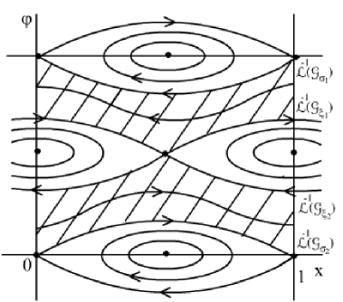
Figure 1: Energy level $E>\frac{1}{2}$

The figure 1 describes the projection these graphs in the section $x\varphi,$ in the energy level $E>\frac{1}{2}.$ Let us consider the closed 1-forms

$$\eta_{i}=\sqrt{2E}\cos\varphi_{i}\left(x\right)dx+Fdy,i=1,2,$$ (4)

dependent of $E$ and $F.$ Since $\mathcal{L}\left(x,v\right)=\left(x,\left\langle\left(v_{1},v_{2}+\cos\left(2\pi x\right)\right),\cdot\right\rangle\right),$ we have $\mathcal{G}_{\eta_{i},0}=\mathcal{L}\left(x,\sqrt{2E}\cos\varphi_{i},\sqrt{2E}\sin\varphi_{i}\right)$. These graphs compose a local foliation in $T^{\ast}\mathbb{T}^{2}$, then are absorbing graphs. It follows from Theorem 1 that $\beta$ is differentiable at any point of $\partial\alpha\left(\left[\eta_{i}\right]\right),$ where

$$\left[\eta_{i}\right]=\int_{0}^{1}\sqrt{2E}\cos\varphi_{i}\left(x\right)dx+Fdy,$$ (5)

for all $i=1,2,$ $E>\frac{1}{2}$ and $F$ with $\left|F\right|<\sqrt{2E}-1.$ Moreover, by Proposition 14, we conclude that $\alpha$ function is differentiable at $\left[\eta_{i}\right].$

Take $F\rightarrow\sqrt{2E}-1$ by left and $F\rightarrow 1-\sqrt{2E}$ by right in (5), for each $i=1,2$, we obtain four closed 1-forms $\sigma_{1},\sigma_{2},\xi_{1}$ and $\xi_{2}$ whose graphs are the connections of saddle. Therefore $\mathcal{G}_{\sigma_{1},0}\cap\mathcal{G}_{\sigma_{1},0}\neq\emptyset$ and the graphs $\mathcal{G}_{\sigma_{1},0}$ and $\mathcal{G}_{\sigma_{2},0}$ is not absorbing. Moreover, since $\mathcal{G}_{\eta_{i},0}$ are absorbing graphs, $\mathcal{A}_{\left[\eta_{i}\right]}^{\ast}=\mathcal{G}_{\eta_{i},0}.$ Then, by semicontinuity of Aubry set, we obtain $\mathcal{A}_{\left[\sigma_{i}\right]}=\mathbb{T}^{2}$, so $\mathcal{A}_{\left[\sigma_{i}\right]}^{\ast}=\mathcal{G}_{\sigma_{i},0}.$ It follows from ([14], Proposition 6) that $\left[\sigma_{1}\right]$ and $\left[\sigma_{2}\right]$ belong to same flat of $\alpha.$ We obtain, analogously, that $\left[\xi_{1}\right]$ and $\left[\xi_{2}\right]$ belong to same flat of $\alpha.$ This show that $\beta$ is neither differentiable at points of $\partial\alpha\left(\left[\sigma_{i}\right]\right)$ nor at points of $\partial\alpha\left(\left[\xi_{i}\right]\right).$ Actually, the homology classes which belong to $\partial\alpha\left(\left[\sigma_{i}\right]\right)$ and $\partial\alpha\left(\left[\xi_{i}\right]\right)$ are $\pm\sqrt{2E}\left(0,1\right)$. In fact, the intersection $\mathcal{A}_{\left[\sigma_{1}\right]}\cap\mathcal{A}_{\left[\sigma_{2}\right]}$ is the intersection of two graphs given by implicit equation

$$\cos\left(2\pi x\right)+\sqrt{2E}\sin\varphi=\sqrt{2E}-1.$$

Thence $\mathcal{A}_{\left[\sigma_{1}\right]}\cap\mathcal{A}_{\left[\sigma_{2}\right]}$ is the closed curve $\gamma_{1}:t\mapsto\left(\frac{1}{2},\sqrt{2E}t\right).$ In particular, $\gamma_{1}$ belongs to $\mathcal{M}_{\left[\sigma_{1}\right]}\cap\mathcal{M}_{\left[\sigma_{2}\right]}$ which supports the measure $\mu_{1}$ with rotation vector equals $\rho\left(\mu_{1}\right)=\sqrt{2E}\left(0,1\right).$ Analogously, $\mathcal{A}_{\left[\xi_{1}\right]}\cap\mathcal{A}_{\left[\xi_{2}\right]}$ is the closed curve $\gamma_{2}:t\mapsto\left(0,-\sqrt{2E}t\right)$ which supports a probability measure $\mu_{2}$ with $\rho\left(\mu_{2}\right)=-\sqrt{2E}\left(0,1\right).$ Therefore we prove that $\beta$ function is not differentiable at any homology class of the form $\left(0,h_{2}\right).$

Remark 16

Since $H$ and $E$ are first integrals, given two constants $a$ and $b,$ the level set $\left(H,E\right)^{-1}\left(a,b\right)=\left\{\left(x,v\right):H\left(x,v\right)=a,E\left(x,v\right)=b\right\}$ is an absorbing set. Therefore, it follows from Proposition 6 that if $H\left(\widetilde{\mathcal{A}}_{c}\right)=F$ for some $c\in H^{1}\left(\mathbb{T}^{2};\mathbb{R}\right),$ then $\left(H,E\right)^{-1}\left(F,\alpha\left(c\right)\right)$ projects onto the whole torus $\mathbb{T}^{2}.$

By previous remark, for all $c\in H^{1}\left(\mathbb{T}^{2};\mathbb{R}\right)$ the Aubry set $\widetilde{\mathcal{A}}_{c}$ is contained in an invariant Lipschitz Lagrangian graph. Since the supports of minimizing measures contained in the graphs $\mathcal{G}_{\sigma_{i},0}$ and $\mathcal{G}_{\xi_{i},0}$ have vector rotation of the form $\left(0,h_{2}\right),$ if $h\in A$ then $\widetilde{\mathcal{M}}^{h}$ is contained in a neighborhood foliated by Lipschitz Lagrangian graphs. It follows from Theorem 15 and Proposition 14 that $\beta$ is of class $C^{1}$ in some neighborhood of $h$ and hence of class $C^{1}$ in $A.$

References

• [1] Arnaud, M-C., The tiered Aubry set for autonomous Lagrangian functions, Ann. Inst. Fourier (Grenoble) 58, no. 5, 1733–1759 (2008).
• [2] Arnaud, M-C., A particular minimization property implies $C^{0}$-integrability, Journal of Differential Equations, 250 (5), 2389-2401 (2011).
• [3] Bernard, P., Contreras, G., A generic property of families of Lagrangian systems, Annals of Mathematics, Pages 1099-1108 from Volume 167 (2008).
• [4] Bernard, P., On the Conley Decomposition of Mather sets, Rev. Mat. Iberoamericana, vol. 26, no. 1, pp. 115–132 (2010).
• [5] Carneiro, M. J., On minimizing measures of the action of autonomous Lagrangians, Nonlinearity, 8 (6): 1077-1085, (1995).
• [6] Carneiro, M. J., Lopes, A., On the minimal action function of autonomous lagrangians associated to magnetic fields, Annales de l’I. H. P., section C, tome 16, N.6, 667-690, (1999).
• [7] Contreras, G., Iturriaga, R., Global Minimizers of Autonomous Lagrangians, CIMAT, México, (2000).
• [8] Contreras, G., Macarini, L., Paternain, G., Periodic Orbits for Exact Magnetic Flows on Surfaces, International Mathematics Research Notices, No. 8, (2004).
• [9] Fathi, A., Weak KAM Theorem and Lagrangian Dynamics Preliminary Version Number 10, (2008).
• [10] Fathi, A., Figalli A., Rifford L., On the Hausdorff dimension of the Mather quotient. Comm. Pure Appl. Math. 62, no. 4, 445-500, (2009).
• [11] Fathi, A., Giuliani, A., Sorrentino, A., Uniqueness of Invariant Lagrangian Graphs in a Homology or a Cohomology Class. Ann. Scuola Norm. Sup. Pisa Cl. Sci. (5) Vol. VIII, 659-680, (2009).
• [12] Mañé, R., Generic properties and problems of minimizing measure of Lagrangian dynamical systems, Nonlinearity, 9, N.2, 273-310, (1996).
• [13] Mañé, R., Global Variational Methods in Conservative Dynamics, IMPA, (1993).
• [14] Massart, D., On Aubry sets and Mather’s action functional, Israel J. Math., 134, 157–71 (2003).
• [15] Massart, D., Vertices of Mather’s Beta function, II, Ergodic Theory Dynam. Systems, 29, no. 4, 1289–1307, (2009).
• [16] Massart, D., Sorrentino, A., Differentiability of Mather’s average action and integrability on closed surfaces, Nonlinearity, 24, 1777–1793, (2011).
• [17] Mather, J. N., Action minimizing invariant measures for positive definite Lagrangian Systems, Math. Zeitschrift, 207, 169-207, (1991).