Magnetar Giant Flares — Flux Rope Eruptions
in Multipolar Magnetospheric Magnetic Fields

Abstract

We address a primary question regarding the physical mechanism that triggers the energy release and initiates the onset of eruptions in the magnetar magnetosphere. A self-consistent stationary, axisymmetric model of the magnetar magnetosphere is constructed based on a force-free magnetic field configuration which contains a helically twisted force-free flux rope. The magnetic field configurations in the magnetosphere are obtained as solutions of an inhomogeneous Grad-Shafranov (GS) equation. Given the complex multipolar magnetic fields at the magnetar surface, we also develop a convenient numerical scheme to solve the GS equation. Depending on the surface magnetic field polarity, there exist two kinds of magnetic field configurations, inverse and normal. For these two kinds of configurations, variations of the flux rope equilibrium height in response to gradual surface physical processes, such as flux injections and crust motions, are carefully examined. We find that equilibrium curves contain two branches, one represents a stable equilibrium branch, the other an unstable equilibrium branch. As a result, the evolution of the system shows a catastrophic behavior: when the magnetar surface magnetic field evolves slowly, the height of flux rope would gradually reach a critical value beyond which stable equilibriums can no longer be maintained. Subsequently the flux rope would lose equilibrium and the gradual quasi-static evolution of the magnetar magnetosphere will be replaced by a fast dynamical evolution. In addition to flux injections, the relative motion of active regions would give rise to the catastrophic behavior and lead to magnetic eruptions as well. We propose that a gradual process could lead to a sudden release of magnetosphere energy on a very short dynamical timescale, without being initiated by a sudden fracture in the crust of the magnetar. Some implications of our model are also discussed.

1 INTRODUCTION

Two intimately connected classes of young neutron stars $-$ Soft Gamma-ray Repeaters (SGRs) and Anomalous X-ray Pulsars (AXPs), which are commonly referred to as magnetars, both show high energy emissions (Mazets et al. 1979; Mereghetti & Stella 1995; Kouveliotou et al. 1998; Gavriil et al. 2002). It is widely believed that the X-ray luminosity in these sources is powered by the dissipation of non-potential (current-carrying) magnetic fields in the ultra-strongly magnetized magnetosphere with the magnetic field $\mathbf{B}$ $\sim 10^{14}-10^{15}$G (Duncan & Thompson 1992; Thompson & Duncan 1996; Thompson et al. 2002). Occasionally, a much brighter outburst has been observed, i.e., a giant flare releases a total energy of $\sim 10^{46}$ergs and has a peak luminosity of $\sim 10^{44-46}$ergs $\mathrm{s}^{-1}$ (for recent reviews see Woods & Thompson 2006; Mereghetti 2008). Although the energy for magnetar outbursts is widely believed to be supplied by the star’s magnetic field, the physical process by which the energy is stored and released remains one of the great puzzles in high-energy astrophysics. Two possibilities exist for the location where the magnetic energy is stored prior to an eruption: in the magnetar crust or in the magnetosphere. For the former possibility, a giant flare may be caused by a sudden untwisting of the internal (to the neutron star) magnetic field (Thompson & Duncan 2001). The subsequent quick and brittle fracture of the crust leads to energetic outbursts. During the outbursts, there would be an enhanced twist of the magnetospheric magnetic field lines. In this crust scenario, the energy stored in the external twist is limited by the tensile strength of the crust. Alternatively, due to the difficulties to explain the short timescale of the giant flare rise time, $\sim$ 0.25 ms (Palmer et al. 2005), the second possibility — the magnetospheric storage model, was proposed by Lyutikov (2006). In this particular scenario, the energy stored in the external twist need not be limited by the tensile strength of the crust, but instead by the total external magnetic field energy (Yu 2011b). In the magnetospheric storage model, the magnetic energy storage processes take place quasi-statically on a longer timescale than the dynamical flare timescale prior to the eruption.

In the magnetospheric model for giant flares, the energy released during an eruption is built up gradually in the magnetosphere before the eruption. Some interesting properties about the storage of magnetic energy of the magnetospheric models have been discussed in Yu (2011b). But there still remains a primary question regarding magnetospheric models, i.e., what is the mechanism that triggers the energy release and initiates the eruption? More specifically, how a very gradual process by the flux injections (Kluźniak & Ruderman 1998; Thompson et al. 2002) or crust motions (Ruderman 1991) could lead to a sudden release of magnetosphere energy on a very short dynamical timescale, without being initiated by a sudden fracture in the rigid component of the neutron star. This catastrophic behavior is essentially reminiscent of solar flares and coronal mass ejections (CMEs). It is conceivable that the magnetosphere adjusts quasi-statically in response to the slowly-changing boundary conditions at the magnetar surface. After reaching a critical point, the magnetosphere could no longer maintain a stable equilibrium and a sudden reconfiguration of the magnetic field occurs due to loss of equilibrium (Forbes & Isenberg 1991; Isenberg et al. 1993; Forbes & Priest 1995). The subsequent physical processes would proceed on a dynamical time scale. This catastrophic process naturally explains the puzzle how a very slow process could lead to the sudden release of external magnetic energy on a much shorter timescale (Thompson et al. 2002).

The magnetar giant flares may involve a sudden loss of equilibrium in the magnetosphere, in close analogy to solar flares and CMEs (Lyutikov 2006). A number of CMEs show structures consistent with the ejection of a magnetic flux rope, as has been reported by Chen et al.(1997) and Dere et al. (1999). Hence magnetic flux ropes have been presumed to be typical structures in the solar corona, and their eruptions might be closely related to solar flares and CMEs (Forbes & Isenberg 1991; Isenberg et al. 1993). Similarly, in the magnetar magnetosphere, magnetic flux ropes could be generated due to the pre-flare activity (Götz et al. 2007; Gill & Heyl 2010). As the magnetic flux injects from deep inside the magnetar, the dissipation of the magnetic field may give rise to the precursor activity. The magnetic dissipation of the precursor could also lead to topology changes of the magnetic fields and the formation of a magnetic flux rope. Such a flux rope is also an indispensable ingredient for the radio afterglow observed in SGR1806 (Gaensler et al. 2005; Lyutikov 2006). It is worthwhile to note that the magnetic field interior to the flux rope, which is suspended in the magnetosphere, is helically twisted. It corresponds to a locally twisted feature in the magnetosphere (Thompson et al 2002; Pavan et al. 2009). Such locally twisted flux ropes seem to be more consistent with recent observations, which suggest the presence of localized twist, rather than global twist (e.g. Woods et al. 2007; Perna & Gotthelf 2008).

Observations show a striking feature that the emergence of a strong four-peaked pattern in the light curve of the 1998 August 27 event from SGR 1900+14, which was shown in data from the Ulysses and BeppoSAX gamma-ray detectors (Feroci et al. 2001). These remarkable data may imply that the geometry of the magnetic field was quite complicated in regions close to the star. It is reasonable to infer that, near the magnetar surface, the magnetic field geometry of an SGR/AXP source involves higher multi-poles. The multipolar magnetic field configurations could be readily understood within the magnetar model. Physically speaking, the electric currents, formed during the birth of magnetar, slowly push out from within the magnetar and generate active regions on the magnetar surface. These active regions manifest themselves as the multipolar regions on the magnetar surface. Due to the presence of the active regions, the magnetic field may deviates from a simple dipole configuration near the magnetar surface (Pavan et al. 2009). Our calculations show that multipolar magnetic active regions, especially their relative motions, would have important implications for the catastrophic eruptions of magnetar giant flares (see Section 4).

Motivated by the similarity between giant flares and solar CMEs, Lyutikov (2006) speculated that magnetar giant flares may also be trigged by the loss of equilibrium of a magnetic field containing a twisted flux rope. But no solid calculations about the equilibrium loss of a flux rope in magnetar magnetosphere have been performed yet. In this paper we focus on the possibility of magnetospheric origin for giant flares and propose that the gradual variations at the magnetar surface could lead to fast dynamical processes in the magnetosphere. We will construct a force-free magnetosphere model with a flux rope suspended in the magnetosphere and study the catastrophic behavior of the flux rope in a background multi-polar magnetic field configuration, taking into account the possible effects of flux injections (Kluźniak & Ruderman 1998; Thompson et al. 2002) and crust horizontal motions (Ruderman 1991). We are especially interested in the critical height of the flux rope that can be achieved in our model. In the mean time, we also develop a convenient numerical scheme to solve the inhomogeneous Grad-Shafranov (GS) equation. Since observed magnetars have a very slow rotation rate, we ignore rotation effects throughout this work.

This paper is structured as follows: in Section 2 we describe the basic equations for the force-free magnetosphere model as well as the multipolar boundary conditions. Two possible magnetic configurations are also discussed in this section. In Section 3 we will discuss the internal and external equilibrium constraints in our model. Numerical results about catastrophic behaviors of the magnetosphere in response to flux injections and crust motions are discussed in Section 4. Conclusions and discussions are given in Section 5. Technical details about the force-free magnetosphere magnetic field are given in Appendix A and B.

2 Axisymmetric Force-Free Magnetosphere with Multipolar Boundary Conditions

The magnetic fields in the magnetar magnetosphere are so strong that the inertia and pressure of the plasma could be ignored (Thompson et al. 2002; Yu 2011a). As a result, the magnetosphere is assumed to be in a force-free equilibrium state, in which $\mathbf{J}\times\mathbf{B}=0$. The axisymmetric force-free magnetic field configurations is determined by an inhomogeneous Grad-Shafranov (GS) equation. Throughout this paper, we work in the spherical polar coordinates ($r,\theta,\phi$).

2.1 Force-Free Magnetic Field Containing a Flux Rope

In our magnetosphere model, one of the distinguishing features is that there exists a helically twisted flux rope in the magnetosphere. The precursor of a giant flare could be relevant to the formation of such helically twisted flux ropes (Götz et al. 2007; Gill & Heyl 2010). Due to the presence of the flux rope, the magnetic fields consist of two parts, one is the fields that are inside the flux rope and the other is the fields outside the flux rope.

In our model the magnetic twist of the flux rope is locally confined to the flux rope interior. This is quite different from the globally twisted magnetic field configurations in Thompson et al. (2002) and Beloborodov (2009). They considered a non-potential force-free field where the electric currents permeate through the entire magnetosphere, while our model only contains a electric current in a spatially confined region, i.e., interior to the flux rope. Note that the toroidal flux rope has a minor radius, $r_{0}$, which is small compared to the height of flux rope, $h$, which is actually the major radius of the flux rope. Under such circumstances, the magnetic field produced by the current inside the flux rope can be viewed as that produced by a wire carrying the net current $I$ at the center of the flux rope (Forbes & Priest 1991) and a simple Lundquist (1950) force-free solution could be applied to represent the distribution of current density and magnetic field inside the flux rope. A brief yet self-contained description of the Lundquist solution is given in Appendix A.

Outside the flux rope, the magnetic field is essentially potential, i.e., the field outside the flux rope is non-twisting. In the regions exterior to the flux rope, the steady state axisymmetric magnetic field in the magnetosphere has only poloidal components and can be written as

$${\bf B}=\nabla\Psi\times\nabla\phi\ ,$$ (1)

where $\Psi(r,\theta)$ is the magnetic stream function and $\phi$ is the third component of the spherical polar coordinates. Written explicitly, the magnetic field is

$${\bf B}=\frac{1}{r\sin\theta}\left(\frac{1}{r}\frac{\partial\Psi}{\partial\theta},\ -\frac{\partial\Psi}{\partial r}\right)\ .$$ (2)

The force-free condition can be cast into the standard Grad-Shafranov (GS) equation (Thompson et al. 2002)

$$\frac{\partial^{2}\Psi}{\partial r^{2}}+\frac{\sin\theta}{r^{2}}\frac{\partial}{\partial\theta}\left(\frac{1}{\sin\theta}\frac{\partial\Psi}{\partial\theta}\right)=-(r\sin\theta)\frac{4\pi}{c}J_{\phi}\ ,$$ (3)

where $c$ is the speed of light. The current density $J_{\phi}$ on the right hand side of the above equation is caused by a toroidal force-free magnetic flux rope mentioned above, which is suspended in the magnetosphere at the height, $h$, by force balances. Note that the stream function $\Psi$ is determined simultaneously by the electric current inside the flux rope and boundary conditions at the magnetar surface. The boundary conditions will be discussed separately in next section. The electric current inside the flux rope could be treated as a source term on the right hand side of the above inhomogeneous GS equation. We treat the current density of the flux rope as a circular ring current of the form (Priest & Forbes 2000)

$$J_{\phi}=\frac{I}{h}\ \delta(\cos\theta)\delta(r-h)\ ,$$ (4)

where $I$ is the electric current carried by the flux rope. Similar treatments have been adopted in the coronal mass ejection (CME) studies (Forbes et al. 1991; Lin et al. 1998). It is clear from this equation that the flux rope is located at the equatorial plane ($\theta=\pi/2$) and the flux rope is the only current source in the region $r>r_{s}$, where $r_{s}$ is the magnetar radius (also see Fig. 2).

2.2 Multipolar Boundary Conditions at Magnetar Surface

In order to solve the boundary-value problem associated with the inhomogeneous GS equation (3), we still need to know the boundary condition at the magnetar surface $r=r_{s}$ (where $r_{s}$ is the magnetar radius). We choose $\Psi$ at the magnetar surface $r=r_{s}$ to be

$$\Psi_{s}(r_{s},\mu)=\Psi_{0}\sigma\Theta(\mu)\ ,$$ (5)

where the subscript $s$ denotes the value on the neutron star surface, $\Psi_{0}$ is a constant with magnetic flux dimension, $\sigma$ is a dimensionless quantity that determines the magnitude of the flux at the surface, and $\mu=\cos\theta$. The magnetic field configuration of neutron stars is basically a dipole field. But near the neutron star surface, where the loss of equilibrium occurs, the magnetic field presents much more complex behaviors (Feroci et al. 2001). To simulate multipolar regions on the neutron star surface, we add two Gaussian functions to the usual dipole field and consequently the function $\Theta(\mu)$ in the above equation takes the following form,

$$\Theta(\mu)\equiv(1-\mu^{2})+\exp\left[-\frac{(\mu-\mu_{0})^{2}}{2w^{2}}\right]+\exp\left[-\frac{(\mu+\mu_{0})^{2}}{2w^{2}}\right]\ ,$$ (6)

where $\mu_{0}$ and $w$ are parameters that determine the magnetic flux distributions at the neutron star surface. We take $w=0.001$ throughout this paper. It is worthwhile to note that, according to the parameter $\Psi_{0}$ introduced in Equation (5), a dimensional current can be defined as

$$I_{0}=\frac{\Psi_{0}c}{r_{s}}\ ,$$ (7)

where $r_{s}$ is the radius of the magnetar. Throughout this paper, we scale all lengths by the neutron star radius $r_{s}$, magnetic flux by $\Psi_{0}$ and current by $I_{0}=\Psi_{0}c/r_{s}$. We also define a dimensionless current $J=I/I_{0}$ for later use, where $I$ is the electric current carried by the flux rope (see Section 2.1).

Fig. 1 shows the profile of the flux function $\Theta(\mu)$ in Equation (6). Note that the derivative with respect to $\mu$ gives the radial component of magnetic field at the magnetar surface. This boundary flux distribution is symmetric with respect to the equator $\theta=\pi/2$ or $\mu=0$. In real circumstances, the active regions on magnetars may form much more complicated patterns without any symmetry. For simplicity, we focus in this paper only on systems with such symmetry. The distance between the two active regions is specified by the parameter $\mu_{0}$. The distribution of $\Theta(\mu)$ for three different values of $\mu_{0}=0.1,0.2,$ and $0.3$ are shown in three panels of Fig. 1. It is clear from this figure that, with the increase of $\mu_{0}$, the active regions move away from each other. Another important physical process, flux injections, can be interpreted in terms of the variation of the parameter, $\sigma$, in Equation (5). This kind of variations do not change the shape of $\Theta(\mu)$, but change the magnitude of flux. For instance, if an opposite polarity magnetic flux is injected from below, due to the magnetic cancellation with the pre-existed magnetic flux at the magnetar surface, the absolute value of the parameter $|\sigma|$ might decrease. Some interesting consequences from both kinds of alterations will be explored in this paper (see Section 4).

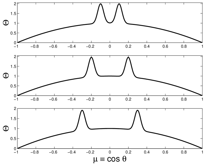
Figure 1: Distribution of magnetic flux at the magnetar surface. Three panels correspond to $\mu_{0}=0.1$, $\mu_{0}=0.2$, and $\mu_{0}=0.3$, respectively. The increase of $\mu_{0}$ clearly shows that the magnetic active regions are moving apart, which will have significant implications for the catastrophic behavior of flux rope.

2.3 Inverse and Normal Configurations

The solution to Equation (3) associated with the boundary condition (5) is of vital importance for our further discussion. With some trivial boundary conditions, this equation can be solved analytically by the Green-function method (Lin et al. 1998). When more complex multipolar boundary conditions, such as Equations (5) and (6), are introduced, this GS equation can generally be solved by the variable separation method. In this paper, we develop a numerical method to solve this equation and full solutions to this inhomogeneous GS equation are given in details in Appendix B.

When solving the GS Equation (3) together with the boundary condition Equations (5) and (6), we find that there exist two kinds of magnetic field configurations in the magnetosphere. One is the the normal configuration, which means that the magnetic field at the position ($r$, $\theta$) = ($h-r_{0}$, $\pi/2$) threads across the flux rope in the same direction as the magnetar surface magnetic field underneath at the equator ($r$, $\theta$) = ($r_{s}$, $\pi/2$). The other is the inverse configuration, in the sense that the magnetic field at the position ($r$, $\theta$) = ($h-r_{0}$, $\pi/2$) threads across the flux rope in the opposite direction to the magnetar surface magnetic field underneath at the equator ($r$, $\theta$) = ($r_{s}$, $\pi/2$). In our calculations, the current $J$ is always kept positive. So for our particular choice of boundary conditions, if $\sigma$ is negative, we will get an normal configuration, if $\sigma$ is positive, an inverse one is obtained. Two schematic figures, both inverse and normal, are shown in the left and right panel of Fig. 2, respectively.

$\begin{array}[]{cc}\includegraphics[width=231.26378pt]{inverse.eps}&\includegraphics[width=231.26378pt]{normal.eps}\\ \end{array}$

Figure 2: Magnetic field lines for both the inverse (left panel) and normal (right panel) magnetic field configurations. Field lines are obtained with solutions of the inhomogeneous GS equation (see Appendix B). The thick black line denotes the magnetar surface. The dashed line is a circle with a radius $r=h$, where $h$ is the height of the flux rope. The flux rope lies at the position ($r$, $\theta$) = ($h$, $\pi/2$). At the magnetar surface $r=r_{s}$, two additional active regions appear due to our choice of boundary conditions.

3 Local-Internal and Global-External Equilibrium Constraints

In what follows, we consider that the magnetar magnetosphere evolves on a sufficiently long timescale so that we can treat the magnetosphere as being essentially in a quasi-static equilibrium. The condition for the flux rope equilibrium includes two parts: the local-internal equilibrium and global-external equilibrium (Forbes & Isenberg 1991).

3.1 Local-Internal Equilibrium Constraints

For the local internal equilibrium, we assume that the force-free condition, $\mathbf{J}\times\mathbf{B}=0$, also applies within the flux rope. We adopt the Lundquist (1950) force-free solution to represent the distribution of current density and field inside the flux rope. For a circular toroidal flux rope in our case, the Lundquist solution inside the flux rope is still valid as long as the minor radius $r_{0}$ is much smaller than the major radius, $h$ (also know as the flux rope height). In this case, a simple relation between the minor radius of the flux rope $r_{0}$ and the current flowing in the flux rope, $I$, can be written as

$$r_{0}=\frac{r_{00}I_{0}}{I}=\frac{r_{00}}{J}\ ,$$ (8)

where $J$ is the dimensionless current scaled by $I_{0}$ and $r_{00}$ is the value for $r_{0}$ as $J=1$. We take $r_{00}=0.01$ throughout this paper. It should be noted that the internal equilibrium constraint, Equation (8), is actually an alternative way indicating the conservation of axial magnetic flux inside the flux rope (see Appendix A).

3.2 Global-external Equilibrium Constraints

The global equilibrium is satisfied when the total force exerted on the flux rope vanishes. The ring current inside the flux rope provides an outward force. Intuitively, the anti-parallel orientation of the current flowing on the opposite sides of the ring produces a repulsive force similar to the force between two parallel wires with anti-parallel currents does. The magnitude of this force is equal to the current, $I$, times the magnetic field $B_{\mathrm{s}}$ (Shafranov 1966):

$$B_{\mathrm{s}}=\frac{I}{ch}\left(\ln\frac{8h}{r_{0}}-1\right)\ ,$$ (9)

where $r_{0}$ is the minor radius of the toroidal flux rope. The additional terms in the bracket of the above equation appear due to the curvature effects of the circular ring current . This ring current induced force must be balanced by the external field $B_{\mathrm{e}}$. The external magnetic field $B_{\mathrm{e}}$ at $r=h$ and $\theta=\pi/2$ can be written explicitly as (The contribution from the current inside the flux loop must be excluded for the external magnetic field $B_{\mathrm{e}}$. For details, see Appendix B)

$$B_{\mathrm{e}}=\sum_{n\ \mathrm{odd}}n\Gamma_{n}d_{n}h^{-n-2}\ ,$$ (10)

where the coefficients $\Gamma_{n}$’s and $d_{n}$’s are all given explicitly in Appendix B. The mechanical equilibrium condition, which requires matching the external field $B_{\mathrm{e}}$ with $B_{\mathrm{s}}$, reads

$$f(\sigma,J,h)=0\ ,$$ (11)

where

$$f(\sigma,J,h)\equiv\left[\sum_{n\ \mathrm{odd}}n\Gamma_{n}d_{n}h^{-n-2}\right]-\frac{J}{h}\left(\ln\frac{8Jh}{r_{00}}-1\right)\ .$$ (12)

Note that the local-internal equilibrium constraint has also been exploited in this equation. Note that the scaled current $J=I/I_{0}$ (not the current $I$) appears in this equation. This is because all quantities, such as $h$, $d_{n}$, and $I$, in this equation are measured in the dimensional units mentioned above (see Section 2.2 and also Appendix B).

The stream function $\Psi$ satisfies the ideal frozen-flux condition, which provides a link between the electric current flowing inside the flux rope and the boundary conditions at the neutron star surface. Specifically, it requires that the stream function on the edge of the flux rope remain constant as the system evolves. At the equator $\theta=\pi/2$, the edge of the flux rope is located at $r=h-r_{0}$ and the frozen-flux condition can be written explicitly as

$$\Psi\left(h-r_{0},\frac{\pi}{2}\right)=\mathrm{const}\ ,$$ (13)

where $h$ and $r_{0}$ are the major and minor radius of the flux rope, respectively. Substituting $r=h-r_{0}$ and $\theta=\pi/2$ into the stream function, i.e., Equation (B1) in Appendix B, we arrive at another constraint,

$$g(\sigma,J,h)=\mathrm{const}\ ,$$ (14)

where

$$g(\sigma,J,h)\equiv\sum_{n\ \mathrm{odd}}\left[\Gamma_{n}c_{n}\left(1-\frac{r_{00}}{Jh}\right)^{n+1}+\Gamma_{n}d_{n}\left(h-\frac{r_{00}}{J}\right)^{-n}\right]\ .$$ (15)

where $d_{n}$’s and $\Gamma_{n}$’s have the same meaning as those in Equation (12), $c_{n}$’s are explicitly given in Appendix A. Note again that all quantities in this equation are measured in the dimensional units defined above. The quantity $r_{00}$ appears because of the internal equilibrium constraint.

In summary the equilibrium constraints, including the force balance and the frozen-flux condition, can be written as the following form

$$\left\{\begin{array}[]{lll}f(\sigma,J,h)=0\\ g(\sigma,J,h)=\mathrm{const}\\ \end{array}\right.\ ,$$ (16)

where functions $f$ and $g$ are defined in Equations (12) and (15). Numerical values of $f$ and $g$ are calculated following the procedures presented in Appendix B. For a given value of $\sigma$, the above two equations could be treated as a nonlinear set of equations for $J$ and $h$, which can be solved numerically by the Newton-Raphson method (Press et al. 1992). Note that the Jacobi matrix necessary for the Newton-Raphson method is hard to obtain analytically and we calculate the Jacobi matrix numerically instead.

4 Loss of Equilibrium in Response to Variations at Magnetar Surface

We consider the possibility that the primary mechanism for driving a magnetar giant flare is a catastrophic loss of equilibrium. The loss of equilibrium is initiated by slow changes at the magnetar surface. Physically, there are generally two possible processes that could occur at the magnetar surface. One is that new magnetic fluxes, driven by the plastic deformation of neutron star crust, may be injected continuously into the magnetosphere (Kluźniak & Ruderman 1998; Thompson et al. 2002; Lyutikov 2006; Götz et al. 2007). Another interesting possibility is brought about by the crust horizontal movement (Ruderman 1991; Jones 2003). It is very difficult to compress magnetar crust material very much, or to move elements of crust up or down. It is, however, much easier to move parts of the crust horizontally, in ways which apply only shear strains to it (Thompson & Duncan 2001; Jones 2003). It is possible that, when the magnetic field is strong enough, the interior magnetic stress may cause the active regions of the crust to move horizontally (Ruderman 1991).

For the first possibility, as the new current-carrying magnetic fluxes are injected, a direct consequence is that the background magnetic field would vary gradually because of the active flux injections prior to large outbursts. The background magnetic field would increase (decrease) if the same (opposite) polarity flux is injected. Variations of the equilibrium height of flux rope with alterations in the background magnetic field are carefully examined for both the inverse and normal magnetic configurations. In this case, we fix the value of $\mu_{0}=0.1$ and investigate the effects of variations of $\sigma$ on the flux rope equilibrium height. Numerical results of Equation (16) are shown in Fig 3. and Fig 4. These two figures show the results for the normal and inverse magnetic configurations, respectively. The curves in Fig. 3 and Fig. 4 consist of two branches, which comes from the fact that there exist two roots of $h$ for each particular value of $\sigma$ and the two roots lie on separate branches. The upper branch denotes an unstable equilibrium state because when the equilibrium is on the upper branch, an slight upward vertical displacement will generate an outward driving force. The lower branch, however, stands for a stable branch, in the sense that an slight upward displacement would create an inward restoring force, just like an harmonic oscillator. The stability of the flux rope could be understood in terms of a spring model. The spring coefficient of Hooke’s law determines the stability of the spring. It would be instructive to treat the total force, $T$, as a function of flux rope height, $h$, while keeping the flux frozen condition satisfied. Detailed analysis shows that derivative $dT/dh$ (which is equivalent to the spring coefficient of Hooke’s law) is negative if the flux rope lies on the lower branch and positive on the upper branch (see Fig. 6.18 in Forbes 2010). Negative $dT/dh$ corresponds to a normal Hooke spring coefficient and a stable equilibrium, while positive $dT/dh$ corresponds to an anomalous Hooke spring coefficient and an unstable equilibrium. The two branches are connected by a critical point (nose point). The instability threshold lies at the nose point. The nose point can also be understood as the critical loss-of-equilibrium point (red point in Fig. 3 and Fig. 4). Once the equilibrium reaches the loss-of-equilibrium critical height, the system would no longer stay in a stable equilibrium state. The flux rope will lose equilibrium and lead to an eruption. In the case of normal configuration, Fig. 3 shows that the increase of the parameter $|\sigma|$ (flux injection of the same polarity) would bring the system to the critical point, which means that the enhancement of the background flux would trigger the catastrophic behavior for a normal configuration. While for the case of inverse configuration, Fig. 4 shows the decrease of the parameter $|\sigma|$ (flux injection of the opposite polarity) would lead to loss of equilibrium, indicating the decay of the background flux works for an inverse configuration. Our calculations show that the critical height for the two kind of configurations differs much. The normal configuration shows a rather low critical height, roughly 3% percent above the magnetar surface, which is, for a typical neutron with radius $10^{6}$cm, roughly $3\times 10^{4}$cm. While for the inverse configuration, the critical height is about 20% above the magnetar surface, which is about $2\times 10^{5}$cm. Given the regular arrangements that occur at the magnetar surface, the small critical height of the normal configuration would indicate that it may not survive those arrangement at the magnetar surface and the inverse configuration, whose critical height is larger, is preferred in real circumstances.

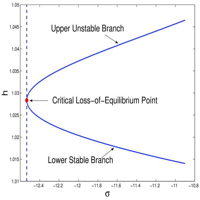
Figure 3: Equilibrium height $h$ as a function of $\sigma$. This curve is numerically obtained as solutions to Equation (16). We always choose the current to be positive. The negative value of $\sigma$ denotes a normal magnetic configuration. In this case, with the increase of of $|\sigma|$, the equilibrium height gradually increases and reaches the critical loss-of-equilibrium point, beyond which the flux rope could not maintain the stable equilibrium. The critical height for the normal magnetic configuration is approximately $h_{c}=1.028$. All lengths are scaled by $r_{s}$.

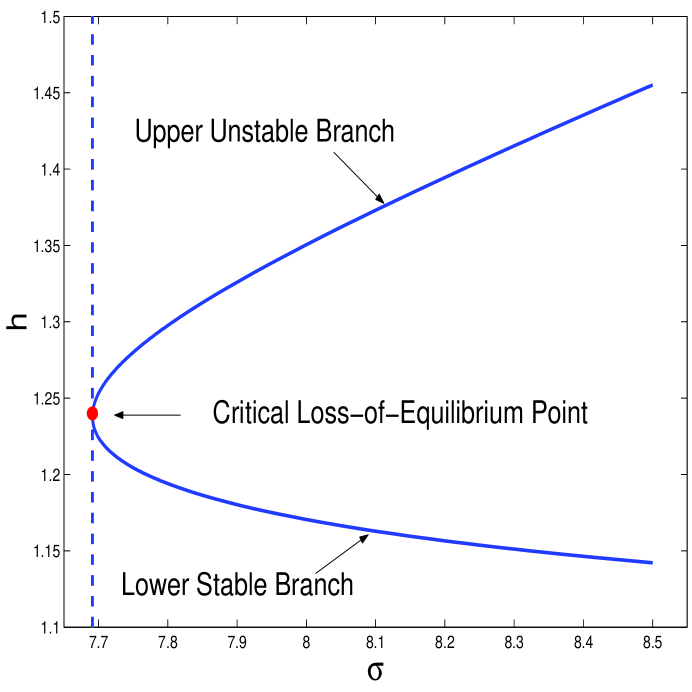
Figure 4: The same as Fig. 3 but for an inverse magnetic field configuration. In this case, with the decrease of of $|\sigma|$, the equilibrium height gradually increases and reaches the critical loss-of-equilibrium point, beyond which the flux rope could not maintain the stable equilibrium. The critical height for normal magnetic configuration is approximately $h_{c}=1.24$. All lengths are scaled by $r_{s}$.

As the interior magnetic stress by the ultra-strong magnetic field in magnetar may cause active regions of the crust to move horizontally (Ruderman 1991; Jones 2003; Lyutikov 2006), the relative positions between multipolar active regions may vary, moving apart or approaching each other, which may also have significant implications for the catastrophic behavior of magnetospheres. Consequently, we further investigate the response of the flux rope to horizontal motions of active regions at the magnetar surface. In our simplified model, the distance between two active regions is determined by a single parameter $\mu_{0}$ in Equation (6). The increase of $\mu_{0}$ may indicate that active regions move apart (see Fig.1). To investigate the effects of horizontal motions, we fix the value of $\sigma$ and vary the parameter $\mu_{0}$. Again, we numerically solve Equation (16) and get two roots of $h$ for each particular value of $\mu_{0}$. We show in Fig. 5, taking the inverse configuration as an example, the variation of the equilibrium height with the distance between two active regions. Similar to Fig. 3 and Fig. 4, the upper branch and the lower branch denotes unstable and stable equilibrium, respectively. As the two active regions move apart, the equilibrium height gradually increases and reaches the critical height $h_{c}=1.32$ when $\mu_{0}=0.14$. After reaching the critical point, the system would no longer maintain a stable equilibrium state. This means that, in addition to flux injections, the horizontal motions of the active regions could give rise to the loss of equilibrium and dynamical eruptions as well.

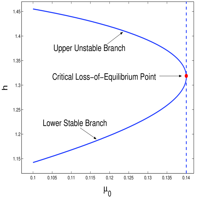
Figure 5: Equilibrium height $h$ as a function of $\mu_{0}$. We fix $\sigma=8.5$ in this figure. With the increase of of $\mu_{0}$, the two active regions move apart. The equilibrium height gradually increases and reaches the critical point, beyond which no stable equilibrium state exists. The critical height for normal magnetic configuration is approximately $h_{c}=1.32$. All lengths are scaled by $r_{s}$.

5 Conclusions and Discussions

In this work, we consider the possibility that the primary mechanism for driving an eruption in magnetar giant flare is a catastrophic loss of equilibrium of a helically twisted flux rope in the magnetar magnetosphere. The loss of equilibrium behavior of a flux rope is investigated in a multi-polar magnetic field configuration, taking into account possible effects of flux injections and crust horizontal motions. The loss of equilibrium model describes a quasi-static equilibrium that varies in response to slow changes at the magnetar surface. Beyond a critical point, the stable equilibrium can not be maintained and the transition to a dynamical evolution naturally occurs.

Equilibrium states of a stationary, axisymmetric magnetic field in the non-rotating magnetosphere containing a flux rope are obtained as solutions of the inhomogeneous GS equation in a spherical polar coordinate. In view of the complex multipolar boundary conditions at the magnetar surface, we develop a numerical method to solve the GS equation. Two kinds of magnetic field configurations, inverse and normal, are carefully examined in this work. Both of them present the loss of equilibrium behavior. We carefully examined the critical height of the flux rope beyond which a stable equilibrium could not be maintained and a sudden release of magnetosphere will be triggered. We find that the critical flux rope height is different for the two types of configurations. We also investigate effects of another form of boundary changes, crust horizontal motions, on the loss of equilibrium behavior. Our results show that both the flux injection and crust motions could trigger the catastrophic behavior in the magnetosphere.

In our simplified model, the flux rope is assumed to be a closed current ring encircling the magnetar. It is suspended in the magnetar magnetosphere and two ends of the flux rope are not anchored to the magnetar surfaces. We expect that the overall catastrophic behavior of our model should remain the same even the anchoring effects of flux rope is taken into account. In order to further understand the anchoring effects on the catastrophic behavior, more realistic three dimensional model that includes a flux rope with two ends anchored to the magnetar surface is worth further investigation.

The magnetic energy that could be released in our model is an interesting issue that is worthwhile to be explored further. For a spherical coordinate in our paper, the ground energy reference state, based on which the fraction of released magnetic energy can be calculated, is the fully open Aly-Sturrock field (Aly 1984, 1991; Sturrock 1991; Yu 2011b). Since the boundary conditions in our paper is more complex (not dipolar or quadrupolar boundary conditions), the construction of the Aly-Sturrock field is technically nontrivial. As a result, the fraction of the energy that could be released in our model involves a very careful calculation of the Aly-Sturrock field. Intuitively, according to prior studies, which have shown that magnetic configurations with more complex boundary conditions would be able to release more energies (Forbes & Isenberg 1991; Isenberg et al. 1993), as well as the complex boundary conditions adopted in our model, it is expected that our model would release enough energy for a magnetar giant flare. Full details of the energetics of our model would be discussed elsewhere.

It is possible that the current sheet forms after the system loses equilibrium (Forbes & Isenberg 1991; Forbes & Priest 1995). With the formation of current sheet, the tearing instability would develop inside the current sheet (Komissarov et al. 2007) and the subsequent magnetic reconnection would further accelerate the flux rope (Priest & Forbes 2000). Magnetic field configurations with the current sheet in a spherical polar coordinate is a long-standing unresolved problem. We note that numerical method developed in this work can be further extended to allow the presence of current sheets (Yu 2011b). Further discussions about the current sheets formation and their effects on the catastrophic behavior would be reported in a separate paper.

It would be interesting to to examine the spectral properties of the model presented in this paper (Thompson et al 2002), in which a locally twisted flux rope is self-consistently incorporated into the magnetar magnetosphere. By fitting the spectral features with observations (Pavan et al. 2009), certain parameters in this model, e.g., flux rope height, electric current and magnetic field, may be better constrained. In parallel, recent Fermi observation of Crab nebulae gamma-ray flare could possibly be explained by the magnetic reconnection models (Abdo et al. 2011), in which the loss of equilibrium may be the trigger for the formation of current sheet and subsequent magnetic reconnection processes. The high energy flare emission from Crab Nebulae is thought to be synchrotron radiation by relativistic electron-positron pairs accelerated in this current sheet (Uzdensky et al. 2011). It would be instructive to calculate, based on the model shown in this paper, the emission spectra and compare them with recent Crab Nebula observations.

The models constructed in this work are likely to be useful as initial states in high resolution force-free electrodynamic numerical simulations to explore the dynamics of magnetic eruptions (Yu 2011a). Our current model can not address the dissipation processes that occur during giant flares. This is left for a future work to directly simulate the behavior of loss of equilibrium and relevant dissipation processes using a newly developed resistive force-free electrodynamic code (Yu 2011a).

Appendix A Lunquist’s solution Interior to Flux Ropes

When the flux rope minor radius is small compared to the major radius of the flux rope, the flux rope interior magnetic field could be approximated as a straight force-free magnetic cylinder. We use Lundquist’s solution to represent the flux rope interior magnetic field. The solution satisfies the force-free condition $\nabla\times\mathbf{B}$ = $\lambda\ \mathbf{B}$, where $\lambda$ is a constant. The solution can be written in a cylindrical coordinate $(r,\theta,z)$. Note that the $z$ direction in this Appendix is actually the $\phi$ direction in the main text. Explicitly, Lundquist’s solution is

$$B_{r}=0\ ,$$ (A1)

$$B_{\theta}=B_{0}J_{1}(\lambda r)\ ,$$ (A2)

$$B_{z}=B_{0}J_{0}(\lambda r)\ ,$$ (A3)

where $B_{z}$ is along the central axis, $B_{\theta}$ is the azimuthal component, and $B_{r}$ is the radial component, $J_{0}$ and $J_{1}$ are the zeroth- and first-order Bessel functions. The conservation of the toroidal flux simply gives

$$\int^{2\pi}_{0}\int^{r_{0}}_{0}B_{z}rdrd\theta=\mathrm{const}\ .$$ (A4)

Substituting the force-free condition $\lambda B_{z}=4\pi j_{z}/c$, we have that

$$\frac{4\pi}{\lambda c}\int^{2\pi}_{0}\int^{r_{0}}_{0}j_{z}rdrd\theta=\frac{4\pi I}{\lambda c}=\mathrm{const}\ ,$$ (A5)

which can be written equivalently as

$$\frac{I}{\lambda}=\mathrm{const}\ .$$ (A6)

At the surface of the flux rope, $B_{z}$ is zero so $J_{0}({\lambda r_{0}})=0$. Therefore $\lambda r_{0}$ is the first zero of $J_{0}$ and $\lambda r_{0}=2.405$. We can finally arrive at

$$r_{0}I=\mathrm{const}\ ,$$ (A7)

which is Equation (8) in the main text.

Appendix B General Solution of the inhomogeneous Grad-Shafranov Equation with Multipolar Boundary Conditions

According to the variable separation method, the general solution to the Grad-Shafranov equation can be written as (see Yu 2011b)

$$\Psi=\sum_{n\ \mathrm{odd}}\left(c_{n}R_{n}(r)+d_{n}r^{-n}\right)\left[\frac{P_{n-1}(\mu)-P_{n+1}(\mu)}{2n+1}\right]\ ,\ \mathrm{n=odd}\ ,$$ (B1)

where $c_{n}$ and $d_{n}$ are constant coefficients to be specified, $P_{n-1}(\mu)$ and $P_{n+1}(\mu)$ are Legendre polynomials, $\mu=\cos\theta$. Here the piece-wise continuous function $R_{n}(r)$ in the above equation is defined as

$$R_{n}(r)=\left\{\begin{array}[]{ll}\left(r/h\right)^{n+1}&r\leq h\\ \left(h/r\right)^{n}&r\geq h\\ \end{array}\right.\ .$$ (B2)

Note that the derivative of the function $R_{n}(r)$ is discontinuous. This feature is exploited in the following to handle the inhomogeneous source terms associated with the Dirac-$\delta$-type current density. Also note an identity for the Legendre polynomials

$$\frac{P_{n-1}(\mu)-P_{n+1}(\mu)}{2n+1}=\frac{(1-\mu^{2})}{n(n+1)}\frac{dP_{n}}{d\mu}\ .$$ (B3)

The inhomogeneous Grad-Shafranov (GS) equation reads

$$\frac{\partial^{2}\Psi}{\partial r^{2}}+\frac{\sin\theta}{r^{2}}\frac{\partial}{\partial\theta}\left(\frac{1}{\sin\theta}\frac{\partial\Psi}{\partial\theta}\right)=-r\sin\theta\frac{4\pi}{c}J_{\phi}\ .$$ (B4)

Substituting Equation (B1) and the explicit expression of $J_{\phi}$ (Equation (4)) into the inhomogeneous GS equation, we arrive at

$$\sum_{n}c_{n}\frac{(1-\mu^{2})}{n(n+1)}\frac{dP_{n}}{d\mu}\left[\frac{d^{2}R_{n}}{dr^{2}}-n(n+1)\frac{R_{k}}{r^{2}}\right]=-r\sin\theta\ \frac{4\pi I}{hc}\ \delta(\cos\theta)\delta(r-h)\ .$$ (B5)

Integrating $r$ over an infinitesimally thin shell around $r=h$, we can rewrite the above equation as

$$\sum_{n}c_{n}\frac{(1-\mu^{2})}{n(n+1)}\frac{dP_{n}}{d\mu}\left[-(2n+1)\frac{1}{h}\right]=-\frac{4\pi I}{c}\sin\theta\delta(\cos\theta)\ .$$ (B6)

Multiplying $\sin\theta\frac{dP_{n}}{d\mu}$ on both sides of the above equation and integrating $\theta$ over $[0,\pi]$ , we have that

$$c_{n}=\left[\frac{(-1)^{\frac{n-1}{2}}n!}{2^{n}\left(\frac{n-1}{2}\right)!\left(\frac{n-1}{2}\right)!}\right]\frac{4\pi Ih}{c}\ .$$ (B7)

It is more convenient to calculate $c_{n}$ numerically by the following recursive relation,

$$c_{1}=0.5\ \left(\frac{4\pi Ih}{c}\right)\ ,\ c_{n+2}=-\left(\frac{n+2}{n+1}\right)\ c_{n}\ .$$ (B8)

Note that terms in the stream function involving $c_{n}$’s are induced by the current inside the flux rope and the external magnetic field in Equation (10) only involves terms related to $d_{n}$’s in Equation (B1). According to Equation (2), the external magnetic field $B_{\mathrm{e}}$ at $r=h$ and $\theta=\pi/2$, can be written explicitly as

$$B_{\mathrm{e}}=\sum_{n\ \mathrm{odd}}n\Gamma_{n}d_{n}h^{-n-2}\ ,$$ (B9)

where

$$\Gamma_{n}=\left[\frac{P_{n-1}(\mu=0)-P_{n+1}(\mu=0)}{2n+1}\right]\ .$$ (B10)

The coefficient $\Gamma_{n}$ can be readily calculated as

$$\Gamma_{1}=0.5\ ,\ \Gamma_{n+2}=-\left(\frac{n}{n+3}\right)\Gamma_{n}\ .$$ (B11)

To specify the coefficients of $d_{n}$’s, we have to take into account the boundary conditions at the magnetar surface. We require that the stream function $\Psi$ be equal to $\Psi_{s}$, i.e., the boundary conditions (5) at the neutron star surface $r=r_{s}$. To achieve this, we expand $\Psi_{s}(\mu)$ as the following

$$\Psi_{s}(\mu)=\sum_{n}a_{n}\left[\frac{P_{n-1}(\mu)-P_{n+1}(\mu)}{2n+1}\right]\ .$$

The coefficients $a_{n}$’s can be expressed as

$$a_{n}=\frac{2n+1}{2}\Psi_{0}\sigma\int^{1}_{-1}\Theta(\mu)\ \frac{dP_{n}(\mu)}{d\mu}d\mu\ .$$

Finally the coefficients $d_{n}$’s can be obtained as follows,

$$d_{n}=r_{s}^{n}\left[a_{n}-c_{n}\left(\frac{r_{s}}{h}\right)^{n+1}\right]\ .\$$ (B12)

For numerical conveniences, we scale all lengths by $r_{s}$, the magnetic flux by $\Psi_{0}$ and the current by $I_{0}=\Psi_{0}c/r_{s}$ throughout this paper. Then the equation $B_{\mathrm{e}}=B_{\mathrm{s}}$ becomes

$$f(\sigma,J,h)=0\ ,$$ (B13)

where

$$f(\sigma,J,h)\equiv\sum_{n\ \mathrm{odd}}n\Gamma_{n}d_{n}h^{-n-2}-\frac{J}{h}\left(\ln\frac{8Jh}{r_{00}}-1\right)\ ,$$ (B14)

and $J=I/I_{0}\$. Similarly the frozen-flux condition can be written as

$$g(\sigma,J,h)\equiv\sum_{n\ \mathrm{odd}}\Gamma_{n}c_{n}\left(1-\frac{r_{00}}{Jh}\right)^{n+1}+\Gamma_{n}d_{n}\left(h-\frac{r_{00}}{J}\right)^{-n}=\mathrm{const}\ .$$ (B15)

Here we can see that both $c_{n}$’s and $d_{n}$’s are explicitly specified and the solution to the inhomogeneous GS equation associated with the multipolar boundary conditions is uniquely determined. The results in this Appendix establish the basis for further investigations of the evolution of the whole system in the main text.

References

- Abdo (2011) Abdo, A. A., et al. 2011, Science, 331, 739
- Aly (1984) Aly, J. J., 1984, ApJ, 283, 349
- Aly (1991) Aly, J. J., 1991, ApJL, 375, 61
- (4) Beloborodov, A. M. 2009, ApJ, 703, 1044
- Chen et al. (1997) Chen, J., et al. 1997, ApJL, 490, 191
- Dere et al. (1999) Dere, K. P., et al. 1999, ApJ, 516, 415
- Duncan & Thompson (1992) Duncan, R. C., & Thompson, C., 1992, ApJL, 392, 9
- Feroci et al. (2001) Feroci, M., Hurley, K., Duncan, R. C., & Thompson, C. 2001, ApJ, 549, 1021
- Forbes (2010) Forbes, T. G. Heliophysics: Space Storms and Radiation: Causes and Effects, 2010, Edited by Carolus, J. S. & George, L. S. (Cambridge Univ. Press), 159
- Forbes & Isenberg (1991) Forbes, T. G., & Isenberg, P. A. 1991, ApJ, 373, 294
- Forbes & Priest (1995) Forbes, T. G., & Priest, E. R. 1995, ApJ, 446, 377
- Gaensler et al. (2005) Gaensler, B. M., et al. 2005, Nature, 434,104
- Gavriil et al. (2002) Gavriil, F. P., Kaspi, V. M., Woods, P. M. 2002, Nature, 419, 142
- Gill & Heyl (2010) Gill, R., & Heyl, J. S. 2010, MNRAS, 407, 1926
- Götz et al. (2007) Götz, D., Mereghetti, S., & Hurley, K. 2007, Ap&SS, 308, 51
- Isenberg et al. (1993) Isenberg, P. A., Forbes, T. G., & Démoulin, P. 1993, ApJ, 417, 368
- Jones (2003) Jones, P. B. 2003, ApJ, 595, 342
- Kluzniak (1998) Kluźniak, W. & Ruderman, M., 1998, ApJL, 505, 113-117
- Komissarov et al. (2007) Komissarov, S. S., Barkov, M. & Lyutikov M., 2007, MNRAS, 374, 415
- Kouveliotou (1998) Kouveliotou, C., et al. 1998, Nature, 393, 235
- Levin & Lyutikov (2012) Levin & Lyutikov, arXiv:1204.2605
- Lin et al. (1998) Lin, J., Forbes, T. G., Isenberg, P. A., & Démoulin, P. 1998, ApJ, 504, 1006
- Lundquist (1950) Lundquist, S. 1950, Ark. Fys., 2, 361
- Lyutikov (2006) Lyutikov, M. 2006, MNRAS, 367, 1602
- Mazets et al. (1979) Mazets, E. P., et al. 1979, Nature, 282, 587
- Mereghetti (2008) Mereghetti, S. 2008, A&AR, 15, 225
- Mereghette & Stella (1995) Mereghetti, S. & Stella, L. 1995, ApJL, 442, 17
- Palmer et al. (2005) Palmer, D. M., et al. 2005, Nature, 434, 1107
- Pavan et al. (2009) Pavan, L., Turolla, R., Zane, S., & Nobili, L. 2009, MNRAS 395, 753
- Perna & Gotthelf (2008) Perna, R., & Gotthelf, E. V. 2008, ApJ, 681, 522
- Priest & Forbes (2000) Priest E., & Forbes T. 2000, Magnetic Reconnection. MHD Theory and Applications. Cambridge Univ. Press, Cambridge
- Press et al. (1992) Press, W. H., Teukolsky, S. A., Vetterling, W. T., & Flannery, B. P. 1992, Numerical Recipes in FORTRAN 2nd Ed., Cambrdige Univ. Press, Cambridge
- Ruderman (1991) Ruderman, M. 1991, ApJ, 366, 261
- Shafranov (1966) Shafranov, V. D. 1966, Rev. Plasma Phys., 2, 103
- Sturrock (1991) Sturrock, P. A. 1991, ApJ, 380, 655
- Thompson & Duncan (1996) Thompson, C., & Duncan, R. C. 1996, ApJ, 473, 322
- Thompson & Duncan (2001) Thompson, C., & Duncan, R. C. 2001, ApJ, 561, 980
- Thompson et al. (2002) Thompson, C., Lyutikov, M., & Kulkarni, S. R. 2002, ApJ, 574, 332
- Uzdensky (2011) Uzdensky, D. A., Cerutti, B. & Begelman, M. C. 2011, ApJL, 737, 40
- van Ballegooijen (1989) van Ballegooijen, A. A., & Martens, P. C. H. 1989, ApJ, 343, 971
- Woods (2001) Woods, P. M., et al., 2001, ApJ, 552, 748
- Woods & Thompson (2006) Woods, P. M., & Thompson, C., 2006, in Compact Stellar X-Ray Sources, ed. W. H. G. Lewin & van der Klis (Cambridge Univ. Press), 547
- Woods et al. (2007) Woods, P. M., et al., 2007, ApJ, 654, 470
- Yu (2011) Yu, C., 2011a, MNRAS, 411, 2461
- Yu (2011) Yu, C., 2011b, ApJ, 738, 75