Phase diagrams of Fermi gases in a trap with mass and population imbalances at finite temperature

Abstract

The pairing and superfluid phenomena in a two-component Fermi gas can be strongly affected by the population and mass imbalances. Here we present phase diagrams of atomic Fermi gases as they undergo BCS–Bose-Einstein condensation (BEC) crossover with population and mass imbalances, using a pairing fluctuation theory. We focus on the finite temperature and trap effects, with an emphasis on the mixture of ⁶Li and ⁴⁰K atoms. We show that there exist exotic types of phase separation in the BEC regime as well as sandwich-like shell structures at low temperature with superfluid or pseudogapped normal state in the central shell in the BCS and unitary regimes, especially when the light species is the majority. Such a sandwich-like shell structure appear when the mass imbalance increases beyond certain threshold. Our result is relevant to future experiments on the ⁶Li–⁴⁰K mixture and possibly other Fermi-Fermi mixtures.

Ultracold Fermi gases provide an excellent model system for studying condensed matter physics, owing to the various experimentally tunable parameters. Using a Feshbach resonance, a two-component Fermi gas of equal spin mixture of atoms of equal mass exhibits a perfect crossover from Bardeen-Cooper-Schrieffer (BCS) type of superfluidity to Bose-Einstein condensation (BEC) Eagles (1969); Leggett (1980); Nozières and Schmitt-Rink (1985), which has been studied intensively both in experiment Zwierlein et al. (2004); Regal et al. (2004); Kinast et al. (2004); Bourdel et al. (2004); Chin et al. (2004) and theory Chen et al. (2005); Giorgini et al. (2008). There have also been a great deal of experimental Partridge et al. (2006a); *Rice2-old; Zwierlein et al. (2006a); *MITPRL06; *Zwierlein2006; *KetterleRF; *MITphase; *Zwierlein2009PRL and theoretical Sheehy and Radzihovsky (2006); De Silva and Mueller (2006); Chien et al. (2006, 2007); Yi and Duan (2006); Chevy and Mora (2010) studies on equal-mass systems with population imbalance. Population imbalance adds a new dimension to the phase diagrams, leading to phase separation Chen et al. (2006), Sarma superfluid Sarma (1963) and possibly Fulde-Ferrell-Larkin-Ovchinnikov (FFLO) states FFL . Mass imbalance, i.e., pairing of different mass atoms, will further enrich the physics. Indeed, there have been world wide efforts on the study of Fermi-Fermi mixture of different species. Over the past several years, Feshbach resonances between different species of fermionic atoms, e.g., ⁶Li and ⁴⁰K, have been found and studied Wille et al. (2008); *Grimm2009PRL; *Grimm2010PRA; *Grimm2011PRL; *Naik; *Grimm2012Nat; Taglieber et al. (2008); *Dieckman2009PRL; *Costa2010PRL; Tiecke et al. (2010), although it remains to achieve superfluidity experimentally. There have been some theoretical studies in this aspect, e.g., on the strong attraction limit at zero temperature $T$ Iskin and Sá de Melo (2008), few-body physics Blume (2012) or the polaron physics Baarsma et al. (2012); Massignan (2012) as well as thermodynamics of a high $T$ normal mixture Daily and Blume (2012). There have also been studies on phase diagrams, which, however, are mostly restricted to zero temperature using a mean field theory either in a homogeneous Fermi gas Iskin and Sá de Melo (2006); Parish et al. (2007) or in a trap Lin et al. (2006); Wu et al. (2006); *Yip2007PRA; Paananen et al. (2007); Guo et al. (2008). Recently, Guo et al. Guo et al. (2009) studied the mass imbalanced Fermi gases at finite temperatures. Due to technical complexity, this study was restricted to homogeneous systems only. In order to address various experiments, which are always done at finite $T$ and in a trap, it is important to take into account the trap and finite temperature effects simultaneously.

In this paper, we consider a two-species Fermi-Fermi mixture with a short-range $s$-wave pairing interaction in a 3D isotropic harmonic trap at finite temperature. We emphasize on the interplay between the finite $T$ Chen et al. (2005, 2007) and trap effects while the mass ratio $m_{\uparrow}/m_{\downarrow}$ and population imbalance (or “spin polarization”) $p=(N_{\uparrow}-N_{\downarrow})/(N_{\uparrow}+N_{\downarrow})$ (as well as the ratio $\omega_{\uparrow}/\omega_{\downarrow}$ between the trapping frequencies) are varied within a pairing fluctuation theory, where spin index $\sigma=\uparrow,\downarrow$ refers to the heavy and light species, respectively. In order to address experiments, we pay special attention to the ⁶Li–⁴⁰K mixture, while keeping in mind other possible mixtures such as ⁶Li–¹⁷³Yb and ¹⁷¹Yb–¹⁷³Yb. We will present our theoretical findings in terms of representative phase diagrams in the $T$–$p$ plane, as long with typical gap and density profiles, throughout the BCS-BEC crossover. One special feature here is the emergence of wide-spread pseudogap phenomena at finite $T$. For high enough mass imbalance, our result shows that, in the $T$–$p$ phase diagrams, three-shell sandwich-like spatial structures occupy a large region both at unitarity and in the BCS regime, including sandwiched phase separation, sandwiched Sarma, sandwiched polarized pseudogap states with increasing $T$. In the BEC regime, there are exotic “inverted” phase separations with a normal Fermi gas core in the trap center surrounded by paired (superfluid or pseudogap) state in the outer shell. Our results provide excellent predictions for future experiments.

Except for slightly different notations, our formalism is a combination of that used in Refs. Guo et al. (2009); Chien et al. (2007), where a single-channel Hamiltonian is used to describe the Fermi gas, with a local density approximation (LDA) for addressing the trap inhomogeneity. The heavy ($\sigma=\uparrow$) and light ($\sigma=\downarrow$) species have dispersion $\xi_{\textbf{k}\sigma}\equiv\epsilon_{\textbf{k}\sigma}-\mu_{\sigma}=k^{2}/2m_{\sigma}-\mu_{\sigma}$, and bare fermion Green’s function $G^{-1}_{0\sigma}(K)=i\omega_{n}-\xi_{\textbf{k}\sigma}$, where $\mu_{\sigma}$ is the chemical potential, $\omega_{n}$ the fermionic Matsubara frequency. As in Ref. Guo et al. (2009), we take $\hbar=k_{B}=1$ and use the four vector notation, e.g., $K\equiv(\omega_{n},\mathbf{k})$, $\sum_{K}\equiv T\sum_{n}\sum_{\mathbf{k}}$, etc. At finite $T$, the self-energy $\Sigma_{\sigma}(K)$ contains two parts, $\Sigma_{\sigma}(K)=\Sigma_{sc,\sigma}(K)+\Sigma_{pg,\sigma}(K)$, where the condensate contribution $\Sigma_{sc,\sigma}(K)=-\Delta_{sc}^{2}G_{0\bar{\sigma}}(-K)$ vanishes above $T_{c}$, and the finite momentum pair contribution $\Sigma_{pg,\sigma}(K)=\sum_{Q}t_{pg}(Q)G_{0\bar{\sigma}}(Q-K)$ persists down to $T=0$. Here $\bar{\sigma}=-\sigma$, and the $T$-matrix $t_{pg}(Q)=g/[1+g\chi(Q)]$ represents an infinite series of particle-particle scattering processes, with a short-range interaction strength $g<0$ and the pair susceptibility $\chi(Q)=\sum_{K,\sigma}G_{0\sigma}(Q-K)G_{\bar{\sigma}}(K)/2$. At and below $T_{c}$, we have $\Sigma_{pg,\sigma}(K)\approx\sum_{Q}t_{pg}(Q)G_{0\bar{\sigma}}(-K)=-\Delta_{pg}^{2}G_{0\bar{\sigma}}(-K)+\delta\Sigma$, which defines a pseudogap $\Delta_{pg}$ via $\Delta_{pg}^{2}\equiv-\sum_{Q}t_{pg}(Q)$. Ignoring the less important incoherent term $\delta\Sigma$, we obtain $\Sigma_{\sigma}(K)=-\Delta^{2}G_{0\bar{\sigma}}(-K)$ in the simple BCS form, where $\Delta^{2}=\Delta_{sc}^{2}+\Delta_{pg}^{2}$. Therefore, the full Green’s function is given by

$$G_{\sigma}(K)=\frac{u_{\textbf{k}}^{2}}{i\omega_{n}-E_{\textbf{k}\sigma}}+\frac{v_{\textbf{k}}^{2}}{i\omega_{n}+E_{\textbf{k}\bar{\sigma}}},$$ (1)

where $u_{\textbf{k}}^{2}=(1+\xi_{\textbf{k}}/{E_{\textbf{k}}})/2$, $v_{\textbf{k}}^{2}=(1-\xi_{\textbf{k}}/{E_{\textbf{k}}})/2$, $E_{\textbf{k}}=\sqrt{\xi_{\textbf{k}}^{2}+\Delta^{2}}$, and $E_{\textbf{k}\sigma}=E_{\textbf{k}}+\zeta_{\textbf{k}\sigma}$, $\xi_{\textbf{k}}=(\xi_{\textbf{k}\uparrow}+\xi_{\textbf{k}\downarrow})/2$, $\zeta_{\textbf{k}\sigma}=(\xi_{\textbf{k}\sigma}-\xi_{\textbf{k}\bar{\sigma}})/2$. With $n_{\sigma}=\sum_{K}G_{\sigma}(K)$, $n=n_{\uparrow}+n_{\downarrow}$ and $\delta n=n_{\uparrow}-n_{\downarrow}$, the number equations read

$$n = \sum_{\textbf{k}}\Big{\{}\Big{(}1-\frac{\xi_{\textbf{k}}}{E_{\textbf{k}}}\Big{)}+2\bar{f}(E_{\textbf{k}})\frac{\xi_{\textbf{k}}}{E_{\textbf{k}}}\Big{\}},$$ (2)

$$\delta n = \sum_{\textbf{k}}\Big{[}f(E_{\textbf{k}\uparrow})-f(E_{\textbf{k}\downarrow})\Big{]},$$ (3)

where the average Fermi function $\bar{f}(x)\equiv\sum_{\sigma}f(x+\zeta_{\textbf{k}\sigma})/2$.

At $T\leq T_{c}$ The Thouless criterion leads to the gap equation $g^{-1}+\chi(0)=0$. For $T>T_{c}$, it is amended by $g^{-1}+\chi(0)=Z\mu_{p}$, where the effective pair chemical potential $\mu_{p}$ and the coefficient $Z$ can be determined from the Taylor expansion of the inverse $T$-matrix Chen et al. (2005), $t_{pg}^{-1}(Q)=Z(i\Omega_{l}-\tilde{\Omega}_{\textbf{q}})$, with $\tilde{\Omega}_{\textbf{q}}=q^{2}/2M^{*}-\mu_{p}$ being the pair dispersion, and $M^{*}$ the effective pair mass. Thus the gap equation reads

$$\frac{m_{r}}{2\pi a}=\sum_{\textbf{k}}\Big{[}\frac{1}{2\epsilon_{\textbf{k}}}-\frac{1-2\bar{f}(E_{\textbf{k}})}{2E_{\textbf{k}}}\Big{]}+Z\mu_{p}\,,$$ (4)

with $\mu_{p}=0$ at $T\leq T_{c}$. Here $g$ is regularized by $g^{-1}=m_{r}/2\pi a-\sum_{\textbf{k}}1/2\epsilon_{\textbf{k}}$, where $a$ is the $s$-wave scattering length, $m_{r}=m_{\uparrow}m_{\downarrow}/(m_{\uparrow}+m_{\downarrow})$ the reduced mass, and $\epsilon_{\textbf{k}}=k^{2}/4m_{r}=\xi_{\mathbf{k}}+\mu$, with $\mu=(\mu_{\uparrow}+\mu_{\downarrow})/2$.

The $T$-matrix expansion leads to the pseudogap equation

$$\Delta_{pg}^{2}=Z^{-1}\sum_{\textbf{q}}b(\tilde{\Omega}_{\textbf{q}}),$$ (5)

where $b(x)$ is the Bose distribution function. As in Ref. Guo et al. (2009), we impose a cutoff $q_{c}$ on the summation such that pairs with $q>q_{c}$ may decay into the particle-particle continuum.

In a harmonic trap, the LDA approximation imposes that the local $\mu_{\sigma}(r)=\mu_{\sigma}(0)-\frac{1}{2}m_{\sigma}\omega_{\sigma}^{2}r^{2}$, with trap frequency $\omega_{\sigma}$. We have the total particle number $N=\int\mathrm{d}^{3}r\,n(r)$ and the number difference $\delta N=N_{\uparrow}-N_{\downarrow}=pN=\int\mathrm{d}^{3}r\,\delta n(r)$. The Fermi energy $E_{F}=(3N)^{1/3}\omega_{\uparrow}=k_{F}^{2}/2m=mR_{TF}^{2}\omega_{\uparrow}^{2}/2=T_{F}$ is defined as that for an unpolarized, noninteracting Fermi gas with the same total number $N$ and trap frequency $\omega_{\uparrow}$, with $m=(m_{\uparrow}+m_{\downarrow})/2$, the average mass. Here $R_{TF}$ is the Thomas-Fermi radius, and the species dependent $R_{TF}^{\sigma}=\sqrt{2(6N_{\sigma})^{1/3}/m_{\sigma}\omega_{\sigma}}$.

For a homogeneous system, Eqs. (2)-(5) form a closed set and can be used to solve for $T_{c}$, as well as $\mu$, $\Delta$, $\Delta_{sc}$ and $\Delta_{pg}$ for given $T$. However, in a harmonic trap, this set of equations have to be solved at each given radius and then subject to the total trap-integrated particle number constraints.

In order to find the stable states in a trap, we compare the (local) thermodynamical potential $\Omega_{S}$ (per unit volume) in a superfluid or pseudogap state with its normal Fermi gas counterpart, $\Omega_{N}=-T\sum_{\textbf{k},\sigma}\ln(1+e^{-\xi_{\textbf{k}\sigma}/T})$. The paired state $\Omega_{S}$ consists of contributions from fermionic excitations $\Omega_{F}$ and noncondensed pairs $\Omega_{B}$:

$$\Omega_{S} = \Omega_{F}+\Omega_{B},$$ (6)

$$\Omega_{F} = -\frac{\Delta^{2}}{g}+\sum_{\textbf{k}}(\xi_{\textbf{k}}-E_{\textbf{k}})-T\sum_{\textbf{k},\sigma}\ln(1+e^{-E_{\textbf{k}\sigma}/T}),$$

$$\Omega_{B} = Z\mu_{p}\Delta^{2}_{pg}+T\sum_{\textbf{q}}\ln(1-e^{-\tilde{\Omega}_{\textbf{q}}/T}).$$

The stable states should have a lower value. When $\Omega_{S}>\Omega_{N}$ at certain radii $r$, phase separation takes place. Note that the $\Omega_{B}$ term is absent in simple mean-field calculations.

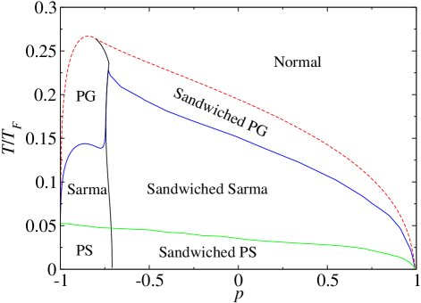
Figure 1: (Color online) $T$–$p$ Phase diagram of ⁶Li-⁴⁰K mixture in a harmonic trap at unitarity, with $\omega_{\uparrow}=\omega_{\downarrow}$. The solid lines separate different phases and the (red) dashed line between the (Sandwiched) PG and the normal phases is approximated by mean field calculations. Here “PG” and “PS” indicate pseudogapped normal state and phase separation, respectively.

Shown in Fig. 1 is the calculated $T$–$p$ phase diagram at unitarity $1/k_{F}a=0$ with $\omega_{\uparrow}=\omega_{\downarrow}$ and mass ratio $m_{\uparrow}/m_{\downarrow}=$ 40:6, as is appropriate for the ⁶Li-⁴⁰K mixture. Corresponding representative density and gap profiles are shown in Fig. 2. It can be seen that phase separation (PS) and sandwiched PS occupy the lowest $T$ part. In particular, when the light species dominates the population, we have a regular phase separation with an equal population superfluid core in the trap center, surrounded by the majority light atoms in the outer shell, similar to that seen in the equal-mass case Chien et al. (2007). Here the gap $\Delta$, the order parameter $\Delta_{sc}$, and the density of minority atoms $n_{\downarrow}$ jump to zero across the interface, as shown in Fig. 2(c). However, except for the light atom dominated case, a three shell structure appears, which we refer to as sandwiched PS. Typical density and gap profiles are shown in Fig. 2(f) (for essentially zero $T$), where an equal population superfluid exists only at intermediate radii, whereas the light and heavy atoms dominate the outer and inner shells, respectively. In fact, at zero $T$, the heavy atoms are absent in the outer shell. The gaps and density profiles exhibit first order jumps at both interfaces. Our findings at the lowest $T$ are consistent with the earlier works at zero temperature Lin et al. (2006); Guo et al. (2008). The primary reason for this three shell structure to occur is that $R_{TF}^{\uparrow}\ll R_{TF}^{\downarrow}$ so that $n_{\uparrow}\gg n_{\downarrow}$ at the trap center. It is known that at low $T$, population imbalance tends to break pairing Chien et al. (2006). Therefore, only at certain intermediate radii where $n_{\uparrow}\approx n_{\downarrow}$ can a superfluid exist. As $p$ decreases from 1 towards -1, these radii move from the trap edge near $R_{TF}^{\uparrow}$ towards the trap center, until the inner shell of normal mixture shrinks to zero around $p=-0.71$.

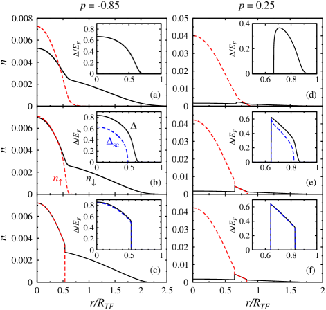
Figure 2: (Color online) Representative density (main panels) and gap (insets) profiles for $p=-0.85$ and 0.25 at unitarity: (a)-(c) $T/T_{F}=0.2$, $0.1$, $0.02$; (d)-(f) $T/T_{F}=0.15$, $0.05$, $0.01$, corresponding to each phase in Fig. 1. The temperatures in (c) and (f) are essentially zero. The (black) solid and (red) dashed lines in the main panels are for ⁶Li ($n_{\downarrow}$, light species) and ⁴⁰K ($n_{\uparrow}$, heavy species), respectively. Plotted in the insets are the total gap $\Delta$ (black solid lines) and order parameter $\Delta_{sc}$ (blue dashed lines). Here the insets share the same x-axes, and the densities $n_{\sigma}$ are in units of $n_{F}\equiv k^{3}_{F}/3\pi^{2}$.

Previous study Chien et al. (2006) demonstrates that in a homogeneous Fermi gas of equal mass at unitarity, a population imbalanced Sarma superfluid Sarma (1963) is stable only at intermediate temperatures. Here we find this remains true for an unequal mass mixture. In Fig. 1, the PS phase becomes a Sarma phase at intermediate $T$, where population imbalance penetrates into the inner superfluid core so that the first order jumps of the gap, the order parameter and the minority density at the interface disappear. This is similar to the Sarma state found in Ref. Chien et al. (2007). Correspondingly, the sandwiched PS phase becomes sandwiched Sarma phase. As seen from the $p=-0.85$ and 0.25 cases shown in Figs. 2(b) and 2(e), respectively, $\Delta$, $\Delta_{sc}$ and $n_{\uparrow}$ vanish continuously at the interface (of the larger radius). The difference between $\Delta$ and $\Delta_{sc}$ defines the presence of the pseudogap (not shown) $\Delta_{pg}=\sqrt{\Delta^{2}-\Delta_{sc}^{2}}$.

As the temperature increases further, the superfluid region disappears so that the Sarma phase becomes a polarized pseudogap (PG) phase, where a finite pseudogap exist in the inner core without superfluidity. In a similar fashion, the sandwiched Sarma phase evolves into a sandwiched PG phase. Representative density and gap profiles are shown in Figs. 2(a) and 2(d) for ($p$, $T/T_{F}$) = (-0.85, 0.2) and (0.25, 0.15), respectively. Finally, at very high $T$ we have a normal phase. Note that the separation between the normal and the PG or sandwiched PG phases is a crossover rather than a phase transition, and thus is determined approximately using the BCS mean-field theory.

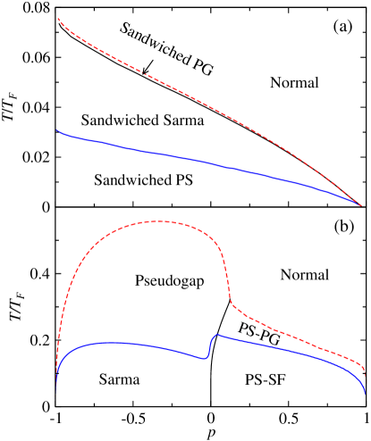
Figure 3: (Color online) Phase diagram of ⁶Li-⁴⁰K as in Fig. 1 but for (a) $1/k_{F}a=-0.5$ and (b) +0.5. Here “PS-SF” and “PS-PG” represent phase separated superfluid and phase separated pseudogap phases, respectively, with a normal gas core surrounded by an outer shell of superfluid or pseudogapped normal mixture.

Next, we present in Fig. 3 the phase diagrams at (a) 1/$k_{F}a$=-0.5 and (b) 0.5, similar to Fig. 1, but in the (near-)BCS and (near-)BEC regimes, respectively. For the BCS case, except for the high $T$ normal phase, the phase diagram is essentially occupied by three-shell sandwich-like structures. The central shell is an unpolarized BCS superfluid at the lowest $T$, spin polarized Sarma superfluid at intermediate $T$, and a polarized pseudogapped normal state at slightly higher $T$. In the sandwiched PS phase, the outer shell is a normal mixture with light species (⁶Li) in excess, surrounded by a single component normal gas of the light atoms at the trap edge. This is different from the sandwiched PS at unitarity [Fig. 2(f)], where the outer shell contains the light atoms only at $T=0$. Typical gap and density profiles (at $p=-0.25$ near $T=0$) are shown in Figs. 4(a) and 4(b), respectively. In comparison with the unitary case, one can see that as the pairing strength decreases from unitarity, the sandwiched PS phase in the phase diagram expands and gradually squeezes out the PS phase completely. The evolution of the various phases with increasing temperature is similar to their unitary counterparts, except that now the sandwiched PG phase occupies a very slim region, reflecting a much weaker pseudogap effect in the BCS regime.

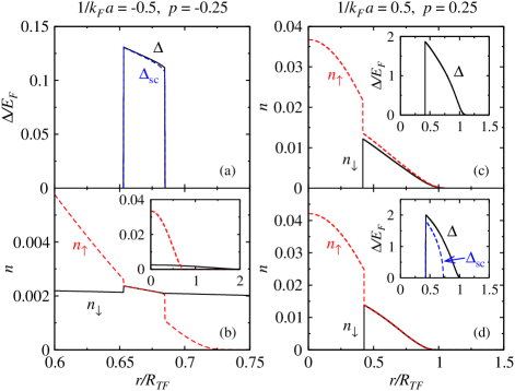
Figure 4: (Color online) Typical density and gap profiles for BCS (left column, $1/k_{F}a=-0.5$) and BEC (right column, $1/k_{F}a=0.5$) regimes. The convention is the same as in Fig. 2. Panels (a) and (b) are for $p=-0.25$ at $T=0.01T_{F}\approx 0$, corresponding to the sandwiched PS phase in Fig. 3(a). Panels (c) and (d) plot the density and gap (insets) distributions for $p=0.25$ at $T=0.2T_{F}$ and $0.1T_{F}$, representing the PS-PG and PS-SF phases in Fig. 3(b), respectively.

The phase diagram for the BEC case in Fig. 3(b) is rather different. First, for $p<0$, where the light species is the majority, a Sarma superfluid phase occurs at low $T$, with essentially equal population at the trap center. Indeed, polarized superfluid becomes stable and phase separation is no longer the ground state in the BEC regime Chien et al. (2006); Chen et al. (2006). As $T$ increases, the order parameter decreases to zero and the system evolves into a polarized pseudogapped normal state. The large area of the “pseudogap” phase indicates greatly enhanced pseudogap effects in the BEC regime. On the other hand, for (roughly) $p>0$, where the heavy species dominates, we have an “inverted” phase separated superfluid state at low $T$, labeled as “PS-SF”, where a normal gas core of the heavy species is surrounded by a shell of unpolarized superfluid. This should be contrasted with the PS phase in the unitary case [Fig. 2(c)], where the normal Fermi gas is outside the superfluid core. As $T$ increases, a phase separated pseudogap state (labeled “PS-PG”) appears, where pseudogap exists in the polarized outer shell but without superfluidity. This is an exotic new phase, which has never been seen or predicted before. Typical density and gap (insets) profiles for the PS-PG and PS-SF phases are shown in Figs. 4(c) and 4(d), respectively. Possible causes for the “inversion” of the phase separation include: (i) For $p>0$, $R_{TF}^{\uparrow}$ of the heavy species becomes close to $R_{TF}^{\downarrow}$ of the light atoms; (2) As the local $k_{F}(r)$ decreases with $r$, the outer region is deeper in the BEC regime than the trap center, making pairing easier and energetically more favorable at the trap edge. When compared with the three-shell structure at unitarity, one concludes that as the pairing strength increases from unitarity, the outer shell of normal light atoms retreats and finally disappears.

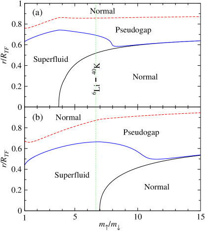
Figure 5: (Color online) Spatial distributions of various phases in the trap at unitarity as a function of mass ratio $m_{\uparrow}/m_{\downarrow}$ for $p=-0.23$ with (a) $T=0.1T_{F}$, $\omega_{\uparrow}=\omega_{\downarrow}$ and (b) $T=0.15T_{F}$ and $\omega_{\downarrow}=2\omega_{\uparrow}$. The (green) dotted line indicates the mass ratio for ⁶Li-⁴⁰K.

We now turn to the case of variable mass ratio $m_{\uparrow}/m_{\downarrow}$, with different $\omega_{\uparrow}/\omega_{\downarrow}$. Plotted in Fig. 5 are spatial distributions of possible phases at unitarity as a function of the mass ratio at $p=-0.23$ for (a) $(T/T_{F},\omega_{\uparrow}/\omega_{\downarrow})=(0.1,1)$ and (b) (0.15, 1/2), respectively. For both cases, a sandwich-like structure appears as the mass ratio increases beyond 3.7 and 7.0, respectively. This can be easily understood by looking at the corresponding non-interacting density distributions Lin et al. (2006). Starting from $m_{\uparrow}/m_{\downarrow}=1$ and $\omega_{\uparrow}/\omega_{\downarrow}=1$, the majority species always has a larger spatial extension so that pairing is easier at the trap center. However, as $m_{\uparrow}/m_{\downarrow}$ becomes sufficiently large, $R_{TF}^{\uparrow}$ of the heavy species may become smaller than $R_{TF}^{\downarrow}$ so that the non-interacting density distribution curves cross each other at an intermediate radius, where pairing is more energetically favorable than elsewhere so that a three-shell structure appears at low $T$, as shown in Fig. 5(a). Note that BCS pairing requires a match of (mass independent) $k_{F}^{\sigma}=(6\pi^{2}n_{\sigma})^{1/3}$ (locally) between the two species. Thus the mass ratio changes the position of the crossing point via changing $R_{TF}^{\sigma}$.

Tuning $\omega_{\uparrow}/\omega_{\downarrow}$ can also change the density crossing point since $R_{TF}^{\sigma}$ depends on the product $m_{\sigma}\omega_{\sigma}$, as shown in Fig. 5(b). This explains why the threshold $m_{\uparrow}/m_{\downarrow}$ for the three-shell structure to occur in Fig. 5(b) is roughly twice that in Fig. 5(a). The (green) vertical dotted line indicates where the ⁶Li–⁴⁰K mixture resides. In this case, a three-shell structure appears in the upper panel while only a regular Sarma phase shows up in the lower panel of Fig. 5.

It is worth pointing out that at large mass imbalance, the strong disparity between $R_{TF}^{\uparrow}$ and $R_{TF}^{\downarrow}$ makes population balance or imbalance less important.

We end by noting that we have not included the species dependent, incoherent part of the fermion self energy, which may induce polarons in the mixed normal states, e.g., in the inner core of the three-shell structured phases. However, it is not important for the present study whether or not the minority species in these states form polarons. Following common practice Kadanoff and Martin (1961); Leggett (1980); Nozières and Schmitt-Rink (1985); Belkhir and Randeria (1992); *Randeria1997; Chen et al. (1998); Perali et al. (2004); Ohashi and Griffin ; Hu et al. (2006); Tchernyshyov (1997); Haussmann (1994), we have also neglected the particle-hole channel contributions GMB , which can be roughly approximated by a shift in the pairing interaction strength Yu et al. (2009); Chen . These approximations are expected to modify the phase boundaries only quantitatively. In addition, we have not considered the FFLO states which, in an equal-mass Fermi gas, appears to be of less interest in 3D He et al. (2007); Sheehy and Radzihovsky (2006); Zhang and Duan (2007). Effects of mass imbalance on the FFLO phases will be investigated in a future work.

In summary, we have studied the finite temperature phase diagrams for Fermi gases in a trap with both mass and population imbalances, using a pairing fluctuation theory, with special attention paid to the ⁶Li–⁴⁰K mixture. Unique to our theory are the wide spread pseudogap phenomena and the prediction of exotic phases, e.g., the phase-separated pseudogap phase, which can be tested by measuring the density and gap profiles in the trap. In particular, vortex measurements and rf spectroscopy Chen et al. (2009) may be used to ascertain the superfluid and pseudogapped normal states. In order to compare with concrete experiments, detailed parameters such as $N_{\sigma}$, $\omega_{\sigma}$, etc are needed. Our results can be tested experimentally when such experiments become available in the (near) future.

This work is supported by NSF of China (Grant No. 10974173), the National Basic Research Program of China (Grants No. 2011CB921303 and No. 2012CB927404), and Fundamental Research Funds for Central Universities of China (Program No. 2010QNA3026).

References

- Eagles (1969) D. M. Eagles, Phys. Rev. 186, 456 (1969).
- Leggett (1980) A. J. Leggett, in Modern Trends in the Theory of Condensed Matter (Springer-Verlag, Berlin, 1980), pp. 13–27.
- Nozières and Schmitt-Rink (1985) P. Nozières and S. Schmitt-Rink, J. Low Temp. Phys. 59, 195 (1985).
- Zwierlein et al. (2004) M. W. Zwierlein, C. A. Stan, C. H. Schunck, S. M. F. Raupach, A. J. Kerman, and W. Ketterle, Phys. Rev. Lett. 92, 120403 (2004).
- Regal et al. (2004) C. A. Regal, M. Greiner, and D. S. Jin, Phys. Rev. Lett. 92, 040403 (2004).
- Kinast et al. (2004) J. Kinast, S. L. Hemmer, M. E. Gehm, A. Turlapov, and J. E. Thomas, Phys. Rev. Lett. 92, 150402 (2004).
- Bourdel et al. (2004) T. Bourdel, L. Khaykovich, J. Cubizolles, J. Zhang, F. Chevy, M. Teichmann, L. Tarruell, S. J. Kokkelmans, and C. Salomon, Phys. Rev. Lett. 93, 050401 (2004).
- Chin et al. (2004) C. Chin, M. Bartenstein, A. Altmeyer, S. Riedl, S. Jochim, J. Hecker-Denschlag, and R. Grimm, Science 305, 1128 (2004).
- Chen et al. (2005) Q. J. Chen, J. Stajic, S. N. Tan, and K. Levin, Phys. Rep. 412, 1 (2005).
- Giorgini et al. (2008) S. Giorgini, L. P. Pitaevskii, and S. Stringari, Rev. Mod. Phys. 80, 1215 (2008).
- Partridge et al. (2006a) G. B. Partridge, W. Li, R. I. Kamar, Y. A. Liao, and R. G. Hulet, Science 311, 503 (2006a).
- Partridge et al. (2006b) G. B. Partridge, W. H. Li, Y. A. Liao, R. G. Hulet, M. Haque, and H. T. C. Stoof, Phys. Rev. Lett. 97, 190407 (2006b).
- Zwierlein et al. (2006a) M. W. Zwierlein, A. Schirotzek, C. H. Schunck, and W. Ketterle, Science 311, 492 (2006a).
- Shin et al. (2006) Y. Shin, M. W. Zwierlein, C. H. Schunck, A. Schirotzek, and W. Ketterle, Phys. Rev. Lett. 97, 030401 (2006).
- Zwierlein et al. (2006b) M. W. Zwierlein, C. H. Schunck, A. Schirotzek, and W. Ketterle, Nature (London) 442, 54 (2006b).
- Schunck et al. (2007) C. H. Schunck, Y. Shin, A. Schirotzek, M. W. Zwierlein, and W. Ketterle, Science 316, 867 (2007).
- Shin et al. (2008) Y. I. Shin, C. H. Schunck, A. Schirotzek, and W. Ketterle, Nature 451, 689 (2008).
- Schirotzek et al. (2009) A. Schirotzek, C.-H. Wu, A. Sommer, and M. W. Zwierlein, Phys. Rev. Lett. 102, 230402 (2009).
- Sheehy and Radzihovsky (2006) D. E. Sheehy and L. Radzihovsky, Phys. Rev. Lett. 96, 060401 (2006).
- De Silva and Mueller (2006) T. N. De Silva and E. J. Mueller, Phys. Rev. A 73, 051602(R) (2006).
- Chien et al. (2006) C. C. Chien, Q. J. Chen, Y. He, and K. Levin, Phys. Rev. Lett. 97, 090402 (2006).
- Chien et al. (2007) C. C. Chien, Q. J. Chen, Y. He, and K. Levin, Phys. Rev. Lett. 98, 110404 (2007).
- Yi and Duan (2006) W. Yi and L. M. Duan, Phys. Rev. A 73, 031604(R) (2006).
- Chevy and Mora (2010) F. Chevy and C. Mora, Reports on Progress in Physics 73, 112401 (2010).
- Chen et al. (2006) Q. J. Chen, Y. He, C.-C. Chien, and K. Levin, Phys. Rev. A 74, 063603 (2006).
- Sarma (1963) G. Sarma, J. Phys. Chem. Solids 24, 1029 (1963).
- (27) P. Fulde and R. A. Ferrell, Phys. Rev. 135, A550 (1964); A. I. Larkin and Y. N. Ovchinnikov, Zh. Eksp. Teor. Fiz. 47, 1136 (1964) [Sov. Phys. JETP 20, 762 (1965)].
- Wille et al. (2008) E. Wille, F. M. Spiegelhalder, G. Kerner, D. Naik, A. Trenkwalder, G. Hendl, F. Schreck, R. Grimm, T. G. Tiecke, J. T. M. Walraven, et al., Phys. Rev. Lett. 100, 053201 (2008).
- Spiegelhalder et al. (2009) F. M. Spiegelhalder, A. Trenkwalder, D. Naik, G. Hendl, F. Schreck, and R. Grimm, Phys. Rev. Lett. 103, 223203 (2009).
- Spiegelhalder et al. (2010) F. M. Spiegelhalder, A. Trenkwalder, D. Naik, G. Kerner, E. Wille, G. Hendl, F. Schreck, and R. Grimm, Phys. Rev. A 81, 043637 (2010).
- Trenkwalder et al. (2011) A. Trenkwalder, C. Kohstall, M. Zaccanti, D. Naik, A. I. Sidorov, F. Schreck, and R. Grimm, Phys. Rev. Lett. 106, 115304 (2011).
- Naik et al. (2011) D. Naik, A. Trenkwalder, C. Kohstall, F. Spiegelhalder, M. Zaccanti, G. Hendl, F. Schreck, R. Grimm, T. Hanna, and P. Julienne, Eur. Phys. J. D 65, 55 (2011).
- Kohstall et al. (2012) C. Kohstall, M. Zaccanti, M. Jag, A. Trenkwalder, P. Massignan, G. M. Bruun, F. Schreck, and R. Grimm, Nature (London) 485, 615 (2012).
- Taglieber et al. (2008) M. Taglieber, A.-C. Voigt, T. Aoki, T. W. Hänsch, and K. Dieckmann, Phys. Rev. Lett. 100, 010401 (2008).
- Voigt et al. (2009) A.-C. Voigt, M. Taglieber, L. Costa, T. Aoki, W. Wieser, T. W. Hänsch, and K. Dieckmann, Phys. Rev. Lett. 102, 020405 (2009), ibid. 105, 269904 (2010).
- Costa et al. (2010) L. Costa, J. Brachmann, A.-C. Voigt, C. Hahn, M. Taglieber, T. W. Hänsch, and K. Dieckmann, Phys. Rev. Lett. 105, 123201 (2010), ibid. 105, 269903 (2010).
- Tiecke et al. (2010) T. G. Tiecke, M. R. Goosen, A. Ludewig, S. D. Gensemer, S. Kraft, S. J. J. M. F. Kokkelmans, and J. T. M. Walraven, Phys. Rev. Lett. 104, 053202 (2010).
- Iskin and Sá de Melo (2008) M. Iskin and C. A. R. Sá de Melo, Phys. Rev. A 77, 013625 (2008).
- Blume (2012) D. Blume, Rep. Prog. Phys 75, 046401 (2012).
- Baarsma et al. (2012) J. E. Baarsma, J. Armaitis, R. A. Duine, and H. T. C. Stoof, Phys. Rev. A 85, 033631 (2012).
- Massignan (2012) P. Massignan, EuroPhys. Lett. 98, 10012 (2012).
- Daily and Blume (2012) K. M. Daily and D. Blume, Phys. Rev. A 85, 013609 (2012).
- Iskin and Sá de Melo (2006) M. Iskin and C. A. R. Sá de Melo, Phys. Rev. Lett. 97, 100404 (2006).
- Parish et al. (2007) M. M. Parish, F. M. Marchetti, A. Lamacraft, and B. D. Simons, Phys. Rev. Lett. 98, 160402 (2007).
- Lin et al. (2006) G.-D. Lin, W. Yi, and L.-M. Duan, Phys. Rev. A 74, 031604 (2006).
- Wu et al. (2006) S.-T. Wu, C.-H. Pao, and S.-K. Yip, Phys. Rev. B 74, 224504 (2006).
- Pao et al. (2007) C.-H. Pao, S.-T. Wu, and S.-K. Yip, Phys. Rev. A 76, 053621 (2007).
- Paananen et al. (2007) T. Paananen, P. Törmä, and J.-P. Martikainen, Phys. Rev. A 75, 023622 (2007).
- Guo et al. (2008) H. Guo, C.-C. Chien, Y. He, Q. J. Chen, and K. Levin (2008), unpublished.
- Guo et al. (2009) H. Guo, C.-C. Chien, Q. J. Chen, Y. He, and K. Levin, Phys. Rev. A 80, 011601 (2009).
- Chen et al. (2007) Q. J. Chen, Y. He, C.-C. Chien, and K. Levin, Phys. Rev. B 75, 014521 (2007).
- Kadanoff and Martin (1961) L. P. Kadanoff and P. C. Martin, Phys. Rev. 124, 670 (1961).
- Belkhir and Randeria (1992) L. Belkhir and M. Randeria, Phys. Rev. B 45, 5087 (1992).
- Engelbrecht et al. (1997) J. R. Engelbrecht, M. Randeria, and C. A. R. Sá de Melo, Phys. Rev. B 55, 15153 (1997).
- Chen et al. (1998) Q. J. Chen, I. Kosztin, B. Jankó, and K. Levin, Phys. Rev. Lett. 81, 4708 (1998).
- Perali et al. (2004) A. Perali, P. Pieri, L. Pisani, and G. C. Strinati, Phys. Rev. Lett. 92, 220404 (2004).
- (57) Y. Ohashi and A. Griffin, preprint, cond-mat/04102201.
- Hu et al. (2006) H. Hu, X. J. Liu, and P. D. Drummond, Europhys. Lett. 74, 574 (2006).
- Tchernyshyov (1997) O. Tchernyshyov, Phys. Rev. B 56, 3372 (1997).
- Haussmann (1994) R. Haussmann, Phys. Rev. B 49, 12975 (1994).
- (61) L. P. Gorkov and T. K. Melik-Barkhudarov, Sov. Phys. JETP 13, 1018 (1961).
- Yu et al. (2009) Z.-Q. Yu, K. Huang, and L. Yin, Phys. Rev. A 79, 053636 (2009).
- (63) Q. J. Chen, arXiv:1109.2307.
- He et al. (2007) Y. He, C.-C. Chien, Q. J. Chen, and K. Levin, Phys. Rev. A 75, 021602 (2007).
- Zhang and Duan (2007) W. Zhang and L.-M. Duan, Phys. Rev. A 76, 042710 (2007).
- Chen et al. (2009) Q. J. Chen, Y. He, C.-C. Chien, and K. Levin, Rep. Prog. Phys. 72, 122501 (2009).