The all-order equation of the effective gluon mass

Abstract

We present the general derivation of the full non-perturbative equation that governs the momentum evolution of the dynamically generated gluon mass, in the Landau gauge. The entire construction hinges crucially on the inclusion of longitudinally coupled vertices containing massless poles of non-perturbative origin, which preserve the form of the fundamental Slavnov-Taylor identities of the theory. The mass equation is obtained from a previously unexplored version of the Schwinger-Dyson equation for the gluon propagator, particular to the PT-BFM formalism, which involves a reduced number of “two-loop dressed” diagrams, thus simplifying the calculational task considerably. The two-loop contributions turn out to be of paramount importance, modifying the qualitative features of the full mass equation, and enabling the emergence of physically meaningful solutions. Specifically, the resulting homogeneous integral equation is solved numerically, subject to certain approximations, for the entire range of physical momenta, yielding positive-definite and monotonically decreasing gluon masses.

I Introduction

The dynamical generation of a momentum-dependent gluon mass Cornwall (1982) has received particular attention lately, especially in light of the important results obtained from a large number of lattice simulations. Specifically, the observed infrared (IR) finiteness of the gluon propagator and the ghost dressing function (in the Landau gauge), both in $SU(2)$ Cucchieri and Mendes (2007, 2009) and in $SU(3)$ Bogolubsky et al. (2007, 2009); Oliveira and Silva (2009), may be explained in terms of such a nonperturbative mass Aguilar et al. (2008); Rodriguez-Quintero (2010); Pennington and Wilson (2011), which tames the IR divergences of the Green’s functions of the theory (for alternative explanations, see,e.g., Dudal et al. (2008)).

The Schwinger-Dyson equations (SDEs) constitute the most natural framework for studying such a nonperturbative phenomenon in the continuum Binosi and Papavassiliou (2008a, b); Alkofer and von Smekal (2001); Fischer (2006); Braun et al. (2010). In particular, the emergence of IR finite solutions out of the SDE governing the gluon propagator has been studied in detail in a series of works (see e.g.,  Aguilar et al. (2008); Fischer et al. (2009); Rodriguez-Quintero (2011)). Particularly interesting in this context is the question of how to isolate the integral equation that determines the momentum evolution of the gluon mass Aguilar et al. (2011). The main purpose of this work is to present the general derivation of the complete gluon mass equation, employing the full SDE of the gluon propagator.

In order to address this difficult question, we consider the set of modified SDE equations obtained within the general framework arising from the synthesis of the pinch technique (PT) Cornwall (1982); Cornwall and Papavassiliou (1989); Binosi and Papavassiliou (2002a); Binosi and Papavassiliou (2004, 2009) with the background field method (BFM) Abbott (1981), known in the literature as the PT-BFM scheme Aguilar and Papavassiliou (2006); Binosi and Papavassiliou (2008a, b). This becomes possible by virtue of set of powerful relations, known as the background-quantum identities Grassi et al. (2001); Binosi and Papavassiliou (2002b). These all-order relations allow one to express the conventional gluon propagator connecting two quantum ($Q$) gluons in terms of the two additional gluon propagators appearing in the BFM: the propagator connecting two background ($B$) gluons, and the propagator connecting a quantum with a background gluon ($BB$ and $QB$ propagators, respectively). This, in turn, permits one to use the SDE for the $BB$ or $QB$ propagators, which are expressed in terms of the Feynman rules characteristic of the BFM, involving fully dressed vertices that satisfy Abelian-like Ward identities (WIs), instead of the typical Slavnov-Taylor identities (STIs). The main consequence of this formulation is that the resulting SDE may be suitably truncated, without compromising the transversality of the answer. As we will explain in detail in the main body of the article, one gains a considerable advantage by considering the version of the identity connecting the $QQ$ with the $QB$ propagators, instead of the one connecting the $QQ$ with the $BB$ propagators, used in the literature so far. Specifically, the resulting SDE (to be denoted as the “$QB$ version” displays the powerful block-wise transversality property known from the $BB$ case, but has two additional important features: it contains fewer graphs, and the limiting procedure necessary for projecting the result to the Landau gauge is significantly less involved.

Even within this improved framework, one still faces the fundamental question of how to disentangle from the SDE of the entire gluon propagator the part that determines the evolution of the mass from the part that controls the evolution of the “kinetic” term. In this work we present a new unambiguous way for implementing this separation, which exploits to the fullest the characteristic structure of a certain type of vertices that are inextricably connected with the process of gluon mass generation.

Specifically, a crucial condition for obtaining out of the SDEs an IR-finite gluon propagator, without interfering with the gauge invariance (or the BRST symmetry) of the theory, is the existence of a set of special vertices, to be generically denoted by $V$, that are purely longitudinal and contain massless poles, and must be added to the usual (fully-dressed) vertices of the theory. The role of these vertices is two-fold. On the one hand, thanks to the massless poles they contain, they make possible the emergence of a IR finite solution out of the SDE governing the gluon propagator; thus, one invokes essentially a non-Abelian realization of the well-known Schwinger mechanism Schwinger (1962a, b). On the other hand, these same poles act like composite Nambu-Goldstone excitations, preserving the form of the STIs of the theory in the presence of a gluon mass. Recent studies indicate that the strong Yang-Mills dynamics can indeed generate longitudinally-coupled composite (bound-state) massless poles, which subsequently give rise to the required vertices $V$ Aguilar et al. (2012a).

It turns out that the very nature of these vertices furnishes a solid guiding principle for implementing the aforementioned separation between mass and kinetic terms. In particular, their longitudinal structure, coupled to the fact that we work in the Landau gauge, completely determines the $q_{\mu}q_{\nu}$ component of the mass equation; this is tantamount to knowing the full mass equation, given that the answer is transverse (so, the $g_{\mu\nu}$ part is automatically fixed from its $q_{\mu}q_{\nu}$ counterpart). If, instead, one had tried to determine the $g_{\mu\nu}$ part first (or had taken the trace of the full equation, as was done in Aguilar et al. (2011)), one would have been confronted with a much subtler exercise. Specifically, the cancellation of the quadratic divergences, implemented by virtue of a characteristic identity, leads to a nontrivial mixing between the $g_{\mu\nu}$ component of the mass and kinetic terms. Even though this separation can be eventually carried out, it is significantly more involved and delicate than that of the $q_{\mu}q_{\nu}$ components.

As already mentioned, in the present work we include all fully dressed graphs (one and two loops) comprising the corresponding full SDE of the $QB$ propagator. Going beyond the “one-loop” dressed analysis is highly nontrivial, because it requires the introduction of a new $V$-type vertex, never considered before. Specifically, in addition to the $V$s related to the three-gluon vertices, known from the one-loop case, the $V$ vertex associated with the fully-dressed four gluon vertex $BQ^{3}$ must be included in the corresponding “two-loop dressed” diagram. As happens in the one-loop case with the three-gluon $V$, this new four-gluon $V$ vertex must satisfy a very concrete QED-like WI, in order to ensure the transversality of the “two-loop dressed” part of the calculation. Interestingly enough, and again as a consequence of their longitudinal nature and the Landau gauge, the WIs (and in some case the STI) satisfied by all $V$-type vertices involved in this problem is all that one needs for calculating their effects exactly. This fact clearly constitutes an important simplification and bypasses the need to actually construct explicitly the corresponding vertices.

As a consequence of the novel aspects introduced in our approach, the one-loop calculation presented in the first part of our derivation (Section V) proceeds in a far more concise way compared to the corresponding derivation followed in Aguilar et al. (2011), rectifying, in fact, the form of the resulting mass equation. The two-loop contribution is considerably more cumbersome to obtain, and is expressed in terms of a kernel that, in addition to full gluon propagators, involves also the conventional, fully dressed, three gluon vertex ($Q^{3}$). The two-loop part of the mass equation is subsequently simplified by choosing tree-level values for a judicious combination of its ingredients, a fact that allows us to carry out explicitly one of the two integrations over virtual momenta. In order to gain insight on the numerical subtleties associated with this equation, we first consider its limit at vanishing physical momenta, thus converting it into a nonlinear constraint. Already at this level, the contribution from the two-loop part appears to be of paramount importance, having far-reaching consequences for the behavior of the resulting solutions. The detailed numerical solution of the full equation (for arbitrary values of the physical momentum) confirms this impression, revealing the existence of positive-definite and monotonically decreasing solutions.

The article is organized as follows. In Section II we introduce the basic notation, together with some of the most important PT-BFM relations, and explain the derivation and general structure of the $QB$ version of the SDE for the gluon propagator. In Section III we present a brief reminder of the basic elements appearing in the gauge-invariant generation of a gluon mass, with particular emphasis on the role and properties of the $V$ vertices. In Section IV we outline in detail the methodology that allows one to extract from the corresponding SDE two separate equations, one for the mass and one for the kinetic term, and explain the advantage of selecting out the $q_{\mu}q_{\nu}$ component. Section V is dedicated to the concise derivation of the one-loop version of the mass equation. In addition, we explain in passing the reason for the discrepancy with the result given in Aguilar et al. (2011); in addition, a brief discussion on the ghost sector (only “one-loop” in this new SDE version) is included, explaining why the ghost graphs do not affect the mass equation. In Section VI we present the full two-loop calculation, organizing the corresponding technical aspects into various self-contained subsections. In Section VII we present the final form of the integral equation that governs the dynamical mass, and discuss some of its general properties. In addition, we calculate an approximate expression for the new contribution to the kernel of this integral equation, to be used in the ensuing numerical analysis. In Section VIII we solve numerically the integral equation, determine a family of positive-definite and monotonically decreasing solutions, and study their dependence on the value of the strong coupling constant. Finally, our conclusions are presented in Section IX.

II A simpler version of the fundamental SDE

In a general renormalizable $R_{\xi}$ gauge, defined through a linear gauge-fixing function of the Lorentz type (${\cal F}^{a}=\partial^{\mu}A^{a}_{\mu}$), the all-order gluon propagator $\Delta^{ab}_{\mu\nu}(q)=\delta^{ab}\Delta_{\mu\nu}(q)$ and its inverse read

$$i\Delta_{\mu\nu}(q)=-i\left[P_{\mu\nu}(q)\Delta(q^{2})+\xi\frac{q_{\mu}q_{\nu}}{q^{4}}\right];\qquad\Delta^{-1}_{\mu\nu}(q)=i\left[P_{\mu\nu}(q)\Delta^{-1}(q^{2})+(1/\xi)q_{\mu}q_{\nu}\right],$$ (1)

where $\xi$ denotes the gauge-fixing parameter ($\xi=0$ corresponds to the Landau gauge), and

$$P_{\mu\nu}(q)=g_{\mu\nu}-q_{\mu}q_{\nu}/q^{2}\,,$$ (2)

is the dimensionless transverse projector. The scalar form factor $\Delta(q^{2})$ appearing above is related to the all-order gluon self-energy $\Pi_{\mu\nu}(q)$; this latter quantity, as a consequence of the BRST symmetry, is transverse to all orders in perturbation theory, as well as non perturbatively, at the level of the corresponding SDE. One has then

$$q^{\mu}\Pi_{\mu\nu}(q)=0;\qquad\Pi_{\mu\nu}(q)=\Pi(q^{2})P_{\mu\nu}(q).$$ (3)

The nonperturbative dynamics of the gluon propagator in the continuum is governed by the corresponding SDE. As has been explained in detail in a series of articles, the formulation of this dynamical equation in the context of the PT-BFM formalism furnishes certain distinct advantages over the conventional case; most importantly, it permits the systematic truncation of the SDE series, without compromising the BRST symmetry, as captured by (3).

Within the BFM formalism three types of gluon propagator make their appearance, in a natural way: (i) the conventional gluon propagator (two quantum gluons entering, $QQ$), denoted (as above) by $\Delta(q^{2})$; (ii) the background gluon propagator (two background gluons entering, $BB$), denoted by $\widehat{\Delta}(q^{2})$; and (iii) the mixed background-quantum gluon propagator (one background and one quantum gluons entering, $BQ$), denoted by $\widetilde{\Delta}(q^{2})$. These three propagators are related among each other by a set of powerful relations, known as Background-Quantum identities Grassi et al. (2001); Binosi and Papavassiliou (2002b), obtained within the Batalin-Vilkovisky formalism Batalin and Vilkovisky (1977, 1981). Specifically,

$$\Delta(q^{2}) = [1+G(q^{2})]^{2}\widehat{\Delta}(q^{2}),$$

$$\Delta(q^{2}) = [1+G(q^{2})]\widetilde{\Delta}(q^{2}),$$

$$\widetilde{\Delta}(q^{2}) = [1+G(q^{2})]\widehat{\Delta}(q^{2}).$$ (4)

The function $G(q^{2})$, which is instrumental for enforcing these crucial relations, is defined as the $g_{\mu\nu}$ form factor of a special two-point function, given by (see Fig. 1)

$$\Lambda_{\mu\nu}(q) = -ig^{2}C_{A}\int_{k}\!\Delta_{\mu}^{\sigma}(k)D(q-k)H_{\nu\sigma}(-q,q-k,k)$$ (5)

$$= g_{\mu\nu}G(q^{2})+\frac{q_{\mu}q_{\nu}}{q^{2}}L(q^{2}),$$

where $C_{A}$ represents the Casimir eigenvalue of the adjoint representation ($N$ for $SU(N)$), $d=4-\epsilon$ is the space-time dimension, and we have introduced the integral measure

$$\int_{k}\equiv\frac{\mu^{\epsilon}}{(2\pi)^{d}}\!\int\!\mathrm{d}^{d}k,$$ (6)

with $\mu$ the ’t Hooft mass. In addition, $D^{ab}(q^{2})=\delta^{ab}D(q^{2})$ is the ghost propagator, and $H_{\nu\sigma}$ is the gluon-ghost kernel shown. The dressed loop expansion of $\Lambda$ and $H$ is shown in Fig. 1; notice finally that, in the Landau gauge, an important all-order relation exists, which links the form factors $G(q^{2})$ and $L(q^{2})$ to the ghost dressing function $F(q^{2})=q^{2}D(q^{2})$, namely Grassi et al. (2004); Aguilar et al. (2009a, b); Aguilar et al. (2010)

$$F^{-1}(q^{2})=1+G(q^{2})+L(q^{2}).$$ (7)

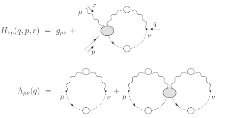
Figure 1: Definitions and conventions of the auxiliary functions $\Lambda$ and $H$. The color and gauge-coupling dependence for the field combination $c^{a}(p)A_{\mu}^{b}(r)A_{\nu}^{*c}(q)$ shown in the $H$ function is $gf^{acb}$. White blobs denote connected Green’s functions, while gray blobs denote one-particle irreducible (with respect to vertical cuts) Schwinger-Dyson kernels.

The basic observation put forth in Aguilar and Papavassiliou (2006); Binosi and Papavassiliou (2008a, b) is that one may use the SDE for $\widehat{\Delta}(q^{2})$, written in terms of the BFM Feynman rules, take advantage of its improved truncation properties, and then convert it to an equivalent equation for $\Delta(q^{2})$ (the propagator simulated on the lattice) by means of the first relation in Eq. (4). The resulting SDE contains a richer diagrammatic structure than the conventional one, due to the appearance of a new subset of graphs, related to the modified ghost sector characteristic of the BFM; specifically, one encounters a new type of ghost vertex, involving two gluons and two ghosts (for the complete set of all relevant Feynman rules, see, for example, Binosi and Papavassiliou (2008b)).

In this article we present an alternative version of the gluon SDE, which displays all known desirable features, and, at the same time, has a reduced diagrammatic complexity. Specifically, instead of using $\widehat{\Delta}(q^{2})$ as the starting point, we consider the SDE satisfied by $\widetilde{\Delta}(q^{2})$, shown in Fig.2, and the second (instead of the first) relation in Eq. (4). Then, the corresponding version of the SDE for the conventional gluon propagator (in the Landau gauge) reads

$$\Delta^{-1}(q^{2}){P}_{\mu\nu}(q)=\frac{q^{2}{P}_{\mu\nu}(q)+i\,\sum_{i=1}^{6}(a_{i})_{\mu\nu}}{1+G(q^{2})},$$ (8)

where the diagrams $(a_{i})$ are shown in Fig. 2.

The crucial points to recognize are (i ) one has a reduced set of Feynman diagrams (six instead of ten) compared to those appearing in the previous formulation in terms of $\widehat{\Delta}(q^{2})$ (six instead of ten, respectively), and (ii ) the most important feature of the PT-BFM formalism for our purposes, namely the block-wise transversality imposed at the level of the SDE for the gluon self-energy, is still present. In particular, the transversality of the gluon self-energy is realized according to the pattern highlighted by the boxes of Fig. 2, namely,

$$q^{\mu}[(a_{1})+(a_{2})]_{\mu\nu}=0;\qquad q^{\mu}[(a_{3})+(a_{4})]_{\mu\nu}=0;\qquad q^{\mu}[(a_{5})+(a_{6})]_{\mu\nu}=0.$$ (9)

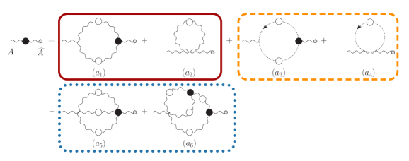
Figure 2: (color online). The SDE obeyed by the $QB$ gluon propagator. Each of the three different boxes (continuous, dashed and dotted line) encloses a set of diagrams forming a transverse subgroup. Black blobs represents fully dressed 1-PI vertices; the small gray circles appearing on the external legs (entering from the right, only!) are used to indicate background gluons.

III Gluon mass generation: a brief reminder

As has been explained in detail in the recent literature, the self-consistent gauge-invariant generation of a gluon mass proceeds through the implementation of the well-known Schwinger mechanism in the context of a Yang-Mills theory. This mechanism requires the existence of a very special type of nonperturbative vertices, to be generically denoted by $V$ (with appropriate Lorentz and color indices], which, when added to the conventional fully dressed vertices have a triple effect: (i ) they make possible that the SDE of the gluon propagator yields $\Delta^{-1}(0)\neq 0$; (ii ) they guarantee that the WIs and STIs of the theory remain intact, i.e., they maintain exactly the same form before and after mass generation; and (iii ) they decouple from on-shell amplitudes. These three properties become possible because the special vertices (a ) contain massless poles and (b ) are completely longitudinally coupled, i.e., they satisfy conditions such as (for the case of the three-gluon vertex)

$$P^{\alpha^{\prime}\alpha}(q)P^{\mu^{\prime}\mu}(r)P^{\nu^{\prime}\nu}(p)\widetilde{V}_{\alpha^{\prime}\mu^{\prime}\nu^{\prime}}(q,r,p)=0.$$ (10)

The origin of the aforementioned poles is due to purely non-perturbative dynamics: for sufficiently strong binding, the mass of certain (colored) bound states may be reduced to zero Jackiw and Johnson (1973); Jackiw (1973); Cornwall and Norton (1973); Eichten and Feinberg (1974); Poggio et al. (1975). In addition to triggering the Schwinger mechanism, these bound-state poles act as composite, longitudinally coupled Nambu-Goldstone bosons, maintaining gauge invariance. Notice, however, that they differ from ordinary Nambu-Goldstone bosons as far as their origin is concerned, since they are not associated with the spontaneous breaking of any continuous symmetry Cornwall (1982). This dynamical scenario has been shown to be realized, within a set of simplified assumptions, through a detailed study in Aguilar et al. (2012a).

For the ensuing analysis it is advantageous to introduce the inverse of the gluon dressing function, to be denoted by $J(q^{2})$. Specifically, in the absence of a gluon mass, we write

$$\Delta^{-1}({q^{2}})=q^{2}J(q^{2}).$$ (11)

From the kinematic point of view we will describe the transition from a massless to a massive gluon propagator by carrying out the replacement (in Minkowski space)

$$\Delta^{-1}(q^{2})=q^{2}J(q^{2})\quad\longrightarrow\quad\Delta_{m}^{-1}(q^{2})=q^{2}J_{m}(q^{2})-m^{2}(q^{2}),$$ (12)

where $m^{2}(q^{2})$ is the (momentum-dependent) dynamically generated mass, and the subscript “$m$” in $J_{m}$ indicates that, effectively, one has now a mass inside the corresponding expressions (i.e., in the SDE graphs).

Gauge invariance requires that the replacement described schematically in Eq. (12) be accompanied by a simultaneous replacement of all relevant vertices by

$$\widetilde{\Gamma}\quad\longrightarrow\quad\widetilde{\Gamma}^{\prime}=\widetilde{\Gamma}_{m}+\widetilde{V},$$ (13)

where $\widetilde{V}$ must be such that the new vertex $\widetilde{\Gamma}^{\prime}$ satisfies the same WIs (or STI) as $\widetilde{\Gamma}$, but now replacing the gluon propagators appearing on their rhs by massive ones.

To see how this works with an explicit example, introducing at the same time some necessary ingredients for the analysis that follows, consider the fully dressed vertex $BQ^{2}$, connecting a background gluon with two quantum gluons, to be denoted by $\widetilde{\Gamma}_{\alpha\mu\nu}$ With the Schwinger mechanism “turned off”, this vertex satisfies the WI

$$q^{\alpha}\widetilde{\Gamma}_{\alpha\mu\nu}(q,r,p)=p^{2}J(p^{2})P_{\mu\nu}(p)-r^{2}J(r^{2})P_{\mu\nu}(r),$$ (14)

when contracted with respect to the momentum of the background gluon. The general replacement described in (13) amounts to introducing the vertex

$$\widetilde{\Gamma}^{\prime}_{\alpha\mu\nu}(q,r,p)=\left[\widetilde{\Gamma}_{m}(q,r,p)+\widetilde{V}(q,r,p)\right]_{\alpha\mu\nu};$$ (15)

then, gauge invariance requires that

$$q^{\alpha}\widetilde{V}_{\alpha\mu\nu}(q,r,p)=m^{2}(r^{2})P_{\mu\nu}(r)-m^{2}(p^{2})P_{\mu\nu}(p),$$ (16)

so that, after turning the Schwinger mechanism on, the corresponding WI satisfied by $\widetilde{\Gamma}^{\prime}$ would read

$$q^{\alpha}\widetilde{\Gamma}^{\prime}_{\alpha\mu\nu}(q,r,p) = q^{\alpha}\left[\widetilde{\Gamma}_{m}(q,r,p)+\widetilde{V}(q,r,p)\right]_{\alpha\mu\nu}$$ (17)

$$= [p^{2}J_{m}(p^{2})-m^{2}(p^{2})]P_{\mu\nu}(p)-[r^{2}J_{m}(r^{2})-m^{2}(r^{2})]P_{\mu\nu}(r)$$

$$= \Delta_{m}^{-1}({p^{2}})P_{\mu\nu}(p)-\Delta_{m}^{-1}({r^{2}})P_{\mu\nu}(r)\,,$$

which is indeed the identity in Eq. (14), with the aforementioned replacement $\Delta^{-1}\to\Delta_{m}^{-1}$ enforced. The remaining STIs, triggered when contracting $\widetilde{\Gamma}^{\prime}_{\alpha\mu\nu}(q,r,p)$ with respect to the other two legs are realized in exactly the same fashion.

Finally, note that “internal” vertices, namely vertices involving only quantum gluons, must be also supplemented by the corresponding $V$, such that their STIs are also unchanged in the presence of masses. To be sure, these vertices do not contain $1/q^{2}$-type of poles, but rather poles in the virtual momenta; therefore, they cannot contribute directly to the mass-generating mechanism. However, they must be included anyway, for gauge invariance to remain intact.

Before concluding this section, it is important to clarify some additional points related to the concepts presented here.

To begin with, a sharp distinction between the notions of “gauge invariance” and “gauge independence” must be established. Gauge invariance is used throughout this work for indicating that a Green’s function satisfies the WI (or STI) imposed by the gauge (or BRST) symmetry of the theory. On the other hand, the gauge (in)dependence of a Green’s function is related with the (independence of) dependence on the gauge-fixing parameter (e.g., $\xi$) used to quantize the theory. Evidently, an off-shell Green’s function may be gauge invariant but gauge dependent: for example, the QED photon-electron vertex, $\Gamma_{\mu}(p,p+q)$, depends explicitly on $\xi$ but satisfies (for every value of $\xi$) the classic WI $q^{\mu}\Gamma_{\mu}(p,p+q)=S^{-1}(p+q)-S^{-1}(p)$. A text-book example of a Green’s function that is both gauge invariant and gauge independent is the photon self-energy (vacuum polarization), which is both transverse and $\xi$ independent.

Evidently, the procedure followed for obtaining the the gluon mass reported in this article (Section VIII) is gauge invariant, because, as explained above, the presence of the vertices $V$ maintains the STIs intact, and the transversality of the $\Pi_{\mu\nu}(q)$ is guaranteed. However, it is clear that a particular gauge choice has been implemented from the beginning, namely that of the Landau gauge. Thus, the gluon mass so derived is particular to that gauge, and we are not aware of any arguments supporting the notion that the same mass would emerge if the SDE analysis were to be repeated, for example, in the Feynman gauge. Therefore, the Landau gauge mass found here should not be considered as an “observable”, in the strict sense of the term. In fact, a qualitatively different picture may appear in the context of different gauge-fixing schemes, such as the Coulomb gauge or the maximal Abelian gauge Kronfeld et al. (1987); for instance, in the former gauge, only “scaling” solutions (for which $\Delta(0)=0$) have been reported Burgio et al. (2010); Watson and Reinhardt (2012).

The mass-generation mechanism employed here (and previous works) hinges crucially on the presence of the special vertices $V$, with the main properties described above. As has been explained in  Jackiw and Johnson (1973); Jackiw (1973); Cornwall and Norton (1973); Eichten and Feinberg (1974); Poggio et al. (1975); Aguilar et al. (2012a), their emergence proceeds through the dynamical formation and subsequent exchange of a massless composite excitation; the massless pole corresponds to the propagator of this excitation. This new amplitude modifies the usual skeleton expansion accordingly, as shown in Fig. 3, given that conventional vertices do not possess such poles. Thus, in that sense, one may interpret the origin of the $V$ vertices as being due to dynamical non-localities in the theory.

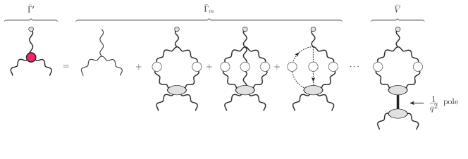
Figure 3: (color online). The $\widetilde{\Gamma}^{\prime}$ three-gluon vertex. Thick gluon lines indicate massive gluons.

It is, therefore, important to recognize the following points.

• These non-localities do not enter at the level of the fundamental QCD Lagrangian, which remains unaltered. In fact, by composite excitation we mean a pole in an off-shell Green’s function representing a field that does not exist in the classical action but that occurs in the solution of the SDE for that Green’s function, as a sort of bound state.

• If one were to describe the $V$ vertices in terms of an effective Lagrangian, one would have indeed to introduce non-localities, as was done in Cornwall (1982); Cornwall and Hou (1986). The resulting theory corresponds to a non-linear sigma model that is non-renormalizable, and can only serve as an approximate low-energy description. We emphasize that we do not use any such model here nor anywhere in the cited works.

• Related to the previous point is the effect that the appearance of such vertices might have on the renormalizability of the Yang-Mills theory. It is clear that no divergences may be introduced that will be in any way proportional to the $V$ vertices, because their renormalization would then require the introduction of non-local terms, and one would effectively end up in the situation described at point (b). The preliminary study Aguilar and Papavassiliou (2010); Binosi and Papavassiliou (2011); Aguilar et al. (2011) of this issue suggests that the $V$ vertices give rise to the gluon mass, with no other residual effects. In fact, eventually, the field-theoretic quantities comprising these vertices are such that the renormalization proceeds identically as that of the conventional part, i.e., through multiplication by the same renormalization constants employed in the massless case.

• Finally, the dynamical equation describing the gluon mass [see Eq. (LABEL:fullmass)] ought to be made finite only through appropriate multiplicative renormalization of its internal substructures, exactly as happens with the dynamical equation (gap equation) describing the momentum evolution of the constituent quark mass Roberts and Williams (1994). The validity of this important property will be assumed in Section VII, when dealing with Eq. (LABEL:fullmass). Note also that, as has been explained in the early works on the subject Cornwall (1982), the renormalizability is intimately related to the vanishing of the gluon mass for large momenta (as seen in our solutions, see Fig.11). Without such large momentum falloff, the SDE would have solutions with extra infinities not corresponding to the perturbative renormalization principles.

IV Deriving the mass equation: General methodology

As explained in the previous section, the special vertices $\widetilde{V}$ (and $V$) enforce the transversality of the rhs of (8) in the presence of gluon masses. Specifically, writing the $\Delta_{m}^{-1}(q^{2})$ on the lhs of Eq. (8) in the form given in Eq. (12), one has that

$$[q^{2}J_{m}(q^{2})-m^{2}(q^{2})]{P}_{\mu\nu}(q)=\frac{q^{2}{P}_{\mu\nu}(q)+i\,\sum_{i=1}^{6}(a_{i}^{\prime})_{\mu\nu}}{1+G(q^{2})},$$ (18)

where the “primes” indicates that (in general) the various fully dressed vertices appearing inside the corresponding diagrams must be replaced by their primed counterparts, as in Eq. (13). Thus, in graph $(a_{1})$ the $BQ^{3}$ vertex will be substituted by $\widetilde{\Gamma}^{\prime}$, while in graph $(a_{6})$ both the $BQ^{2}$ and the $Q^{3}$ type of vertices must contain the corresponding $\widetilde{V}$ and $V$ components, respectively. In addition, in diagram $(a_{5})$ the primed version of the vertex $BQ^{3}$ will make its appearance. These modifications have an important effect: the blockwise transversality property of Eq. (9) holds also for the “primed” graphs, i.e., when $(a_{i})\to(a_{i}^{\prime})$.

The lhs of Eq. (18) involves two unknown quantities, $J_{m}(q^{2})$ and $m^{2}(q^{2})$, which will eventually satisfy two separate, but coupled, integral equations. of the generic type

$$J_{m}(q^{2}) = 1+\int_{k}{\cal K}_{1}(q^{2},m^{2},\Delta_{m}),$$

$$m^{2}(q^{2}) = \int_{k}{\cal K}_{2}(q^{2},m^{2},\Delta_{m}).$$ (19)

such that $q^{2}{\cal K}_{1}(q^{2},m^{2},\Delta_{m})\to 0$, as $q^{2}\to 0$, whereas ${\cal K}_{2}(q^{2},m^{2},\Delta_{m})\neq 0$ in the same limit, precisely because it includes the $1/q^{2}$ terms contained inside the $\widetilde{V}$ terms.

In the present work we will focus on the derivation of the closed form of the integral equation governing $m^{2}(q^{2})$. To that end, we must identify all mass-related contributions contained in the Feynman graphs that comprise the rhs of Eq. (18). Now, with the transversality of both sides of Eq. (18) guaranteed, it turns out that it is far more economical to derive the mass equation by isolating the appropriate cofactors of $q_{\mu}q_{\nu}/q^{2}$ on both sides, instead of the $g_{\mu\nu}$, or instead of taking the trace. In particular, to obtain the rhs of the mass equation, one must (i ) consider the graphs that contain a vertex ${\widetilde{V}}$, and (ii ) isolate the $q_{\mu}q_{\nu}/q^{2}$ component of the contributions coming from the ${\widetilde{V}}$ vertices.

To explain how one reaches the above conclusion, let us first point out that, clearly, in the absence of the $\widetilde{V}$, which contain the massless poles, no gluon mass could be generated; so, the gluon mass is inextricably connected with the $\widetilde{V}$s. In addition, as we will see in detail in what follows, the longitudinal nature of these latter vertices [viz. Eq. (10)], coupled to the fact that we work in the Landau gauge, force the corresponding contribution to the gluon self-energy to be proportional to $q_{\nu}$ [see Eqs. (41) and (64)]. The only exception to this rule is the $V$ that appears inside graph $(a_{6})$, as part of the $Q^{3}$ vertex $\Gamma^{\prime}$; however, the corresponding contribution is shown to vanish identically in the Landau gauge (see Section VI). Thus, if we denote by $(a^{{\scriptscriptstyle\widetilde{V}}}_{i})_{\mu\nu}$ the ${\widetilde{V}}$-related contributions of the corresponding diagrams, these latter terms are proportional to $q_{\mu}q_{\nu}/q^{2}$ only, namely

$$(a^{{\scriptscriptstyle\widetilde{V}}}_{i})_{\mu\nu}=\frac{q_{\mu}q_{\nu}}{q^{2}}a^{{\scriptscriptstyle\widetilde{V}}}_{i}(q^{2}),$$ (20)

so that

$$m^{2}(q^{2})=\frac{i\sum_{i}a_{i}^{{\scriptscriptstyle\widetilde{V}}}(q^{2})}{1+G(q^{2})}\,,$$ (21)

where the sum includes only the graphs $i=1,5,6$.

Similarly, the equation for $J_{m}(q^{2})$ may be obtained from the $q_{\mu}q_{\nu}/q^{2}$ component of the parts of the graphs that do not contain $V$ components. These graphs are identical to the original set $(a_{1})-(a_{6})$, but now $\widetilde{\Gamma}\longrightarrow\widetilde{\Gamma}_{m}$, $\Delta\longrightarrow\Delta_{m}$, etc. To avoid notational clutter we will use the same letter as before, and the aforementioned changes are understood. These contributions may be separated in $g_{\mu\nu}$ and $q_{\mu}q_{\nu}/q^{2}$ components,

$$(a_{i})_{\mu\nu}=g_{\mu\nu}\,{A_{i}}(q^{2})+\frac{q_{\mu}q_{\nu}}{q^{2}}{B_{i}}(q^{2}).$$ (22)

Note that graphs $(a_{2})$ and $(a_{4})$ are proportional to $g_{\mu\nu}$ only; so, in the notation introduced above, $B_{2}(q^{2})=B_{4}(q^{2})=0$. Then, the corresponding equation for $J_{m}(q^{2})$ reads

$$-q^{2}J_{m}(q^{2})=\frac{-q^{2}+i\sum_{i}B_{i}(q^{2})}{1+G(q^{2})},$$ (23)

with $i=1,3,5,6$.

We hasten to emphasize that the fact that we focus on the $q_{\mu}q_{\nu}/q^{2}$ terms, instead of the $g_{\mu\nu}$, in no way indicates a potential clash with the transversality of the gluon self-energy, which is manifestly preserved throughout. In fact, it is precisely the validity of Eq. (3) that allows one to choose freely between the two tensorial structures. The point is that the transversality of Eq. (18) should not be interpreted to mean that the algebraic origin of the terms proportional to $g_{\mu\nu}$ is the same as that of the terms proportional to $q_{\mu}q_{\nu}/q^{2}$. In particular, the $q_{\mu}q_{\nu}/q^{2}$ of $J_{m}(q^{2})$ and $m^{2}(q^{2})$ are easily separable, as the Eqs. (21) and (23) indicate, whereas their $g_{\mu\nu}$ parts are entangled, and their separation is significantly more delicate.

As a particular example of how the $g_{\mu\nu}$ part requires an elaborate treatment, while the $q_{\mu}q_{\nu}/q^{2}$ does not, let us consider the basic cancellation taking place at the one-loop dressed level, enforced by the so-called “seagull identity”: the (quadratic) divergence of the “seagull” diagram ($a_{2}$) is annihilated exactly by a very particular contribution coming from graph ($a_{1}$), by virtue of the identity (valid in dimensional regularization) Aguilar and Papavassiliou (2010)

$$\int_{k}\!k^{2}\frac{\mathrm{d}{\Delta_{m}(k^{2})}}{{\mathrm{d}}k^{2}}+\frac{d}{2}\int_{k}\!\Delta_{m}(k^{2})=0.$$ (24)

The important fact to realize is that all terms involved in the cancellation enforced by Eq. (24) are proportional to $g_{\mu\nu}$, and it is only after they are properly combined that their total contribution vanishes (as $q^{2}\to 0$), by virtue of Eq. (24); instead, their $q_{\mu}q_{\nu}/q^{2}$ counterparts vanish individually, in the same limit.

In order to appreciate this last point, consider the expression

$$I_{\mu\nu}(q)\equiv\int_{k}\!k_{\mu}k_{\nu}f(k,q),$$ (25)

where $f(k,q)$ is an arbitrary function that remains finite in the limit $q^{2}\to 0$. Clearly,

$$I_{\mu\nu}(q)=g_{\mu\nu}{A}(q^{2})+\frac{q_{\mu}q_{\nu}}{q^{2}}B(q^{2})\,,$$ (26)

and the form factors $A(q^{2})$ and $B(q^{2})$ are given by

$$A(q^{2}) = \frac{1}{d-1}\int_{k}\!\left[k^{2}-\frac{(k\cdot q)^{2}}{q^{2}}\right]f(k,q),$$

$$B(q^{2}) = -\frac{1}{d-1}\int_{k}\!\left[k^{2}-d\frac{(k\cdot q)^{2}}{q^{2}}\right]f(k,q).$$ (27)

Then, setting $(q\cdot k)^{2}=q^{2}k^{2}\cos^{2}\theta$, and using that, for any function $f(k^{2})$

$$\int_{k}\!\cos^{2}\theta f(k^{2})=\frac{1}{d}\int_{k}\!f(k^{2}),$$ (28)

we obtain from Eq. (27) that, as $q^{2}\to 0$,

$$A(0)=\frac{1}{d}\int_{k}\!k^{2}\,f(k);\qquad B(0)=0.$$ (29)

Evidently, the function $f$ may be such that the integral defining $A(0)$ diverges, while, for the same function, $B(0)$ vanishes.

Now, in the context of the one-loop dressed calculation, the term $I_{\mu\nu}(q)$ originates from graph $(a_{1})$, with the replacement $\widetilde{\Gamma}\to\widetilde{\Gamma}_{m}$, $\Delta\to\Delta_{m}$, as mentioned above. The WI satisfied by $\widetilde{\Gamma}_{m}$ is that of Eq. (14) with $J\to J_{m}$, and similar but more complicated STIs hold when contracting with respect to the other momenta. Note that what appears in the WI and STIs is $J_{m}$ and not $\Delta_{m}$. Then, as has been shown in Binosi and Papavassiliou (2011), the longitudinal part of $\widetilde{\Gamma}_{m}$ may be expressed in terms of $J_{m}$ (and other Green’s functions), and as a result, the function $f(k)$ (at $q^{2}=0$) is given by

$$f(k^{2})=-\Delta^{2}_{m}(k^{2})\frac{{\mathrm{d}}\left(k^{2}J_{m}(k^{2})\right)}{{\mathrm{d}}k^{2}}.$$ (30)

Now, the point is that, in order to trigger Eq. (24), $f(k^{2})$ should be instead

$$f(k^{2})=-\Delta^{2}_{m}(k^{2})\frac{{\mathrm{d}}\Delta^{-1}(k^{2})}{{\mathrm{d}}k^{2}}=\frac{{\mathrm{d}}\Delta_{m}(k^{2})}{{\mathrm{d}}k^{2}}.$$ (31)

To accomplish this, one adds and subtracts $m^{2}(k^{2})$ to the $f(k)$ of the $A(0)$ given in Eq. (29), thus obtaining

$$A(0)=\frac{1}{d}\left[\int_{k}\!k^{2}\frac{{\mathrm{d}}\Delta_{m}(k^{2})}{{\mathrm{d}}k^{2}}-\int_{k}\!k^{2}\frac{{\mathrm{d}}m^{2}(k^{2})}{{\mathrm{d}}k^{2}}\right].$$ (32)

At that point, the first term on the rhs of Eq. (32) goes to the $g_{\mu\nu}$ part of the equation of $J_{m}(q^{2})$; when added to the term $(a_{2})$, which is also assigned (in its entirety) to the $g_{\mu\nu}$ part of that same equation, it finally gives rise, by virtue of Eq. (24), to a contribution that is free of quadratic divergences and vanishes in the $q^{2}=0$ limit, as it should. On the other hand, the second term on the rhs of Eq. (32) is allotted to the mass equation. Thus, unlike $B(q^{2})$, which unambiguously contributes to the $q_{\mu}q_{\nu}/q^{2}$ part of the equation for $J_{m}(q^{2})$ [and satisfies automatically $B(0)=0$], the $A(q^{2})$ contributes to the $g_{\mu\nu}$ component of both equations.

Let us finally point out that the purely longitudinal nature of the vertices $\widetilde{V}$ (and $V$) expressed through conditions such as Eq. (10), combined with the fact that we work in the Landau gauge, allows one to obtain all relevant contributions simply from the knowledge of the WI (or STI) that these vertices satisfy, without the need to construct them explicitly. This is particularly important in the case of the vertex $\widetilde{V}_{\nu\rho\sigma\tau}$, appearing in graph $(a_{5})$; indeed, constructing this vertex explicitly would constitute an arduous task, given the complicated STIs that it satisfies when contracted by the momentum of any of its three quantum legs.

V The “one-loop dressed” mass equation: Concise derivation

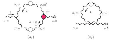
Figure 4: (color online). The one-loop dressed part of the SDE that contains only gluons. Thick lines represent, as previously exlpained, gluon propagators endowed with a momentum-dependent mass. The fully dressed primed vertex, $\widetilde{\Gamma}^{\prime}$, enforces gauge invariance in the presence of such a mass. The symmetry factor is $1/2$ in both cases. We also show for the reader’s convenience (in this and the next figures) the color and Lorentz indices, as well as the momentum routing used in our calculations.

According to the methodology outlined in the previous section, the one-loop dressed contribution to the gluon mass equation stems solely from the $\widetilde{V}$-part of graph $(a_{1}^{\prime})_{\mu\nu}$, to be denoted by $(a^{{\scriptscriptstyle\widetilde{V}}}_{1})_{\mu\nu}$.

The first simplification stemming from the use of the SDE for the $QB$ propagator (as opposed to the $BB$ employed in Aguilar et al. (2011)) is that the Landau gauge limit $\xi=0$ may be taken directly, in the part of the calculation related to the masses. Indeed, the only source of terms proportional to $\xi^{-1}$ (which require special care) is the tree-level part of the $BQ^{2}$ vertex, which only affect the equation for $J(q^{2})$ (and can be easily dealt with, following the procedure explained in Aguilar et al. (2008)). Then (see Fig. 4 for the Lorentz and color indices as well as the momenta routing used in the following calculation)

$$(a^{{\scriptscriptstyle\widetilde{V}}}_{1})_{\mu\nu}=\frac{1}{2}\,g^{2}C_{A}\int_{k}\!{\Gamma}^{(0)}_{\mu\alpha\beta}(q,k,-k-q)\Delta^{\alpha\rho}(k)\Delta^{\beta\sigma}(k+q)\widetilde{V}_{\nu\rho\sigma}(q,k,-k-q)\,,$$ (33)

where ${\Gamma}^{(0)}_{\mu\alpha\beta}$ is the conventional three-gluon vertex of the linear covariant gauges,

$${\Gamma}^{(0)}_{\mu\alpha\beta}(q,k,-k-q)=(q-k)_{\beta}\,g_{\mu\alpha}+(2k+q)_{\mu}\,g_{\alpha\beta}-(2q+k)_{\alpha}\,g_{\beta\mu},$$ (34)

and $\Delta_{\alpha\beta}(k)$ is the totally transverse Landau gauge propagator, namely

$$\Delta_{\alpha\beta}(k)=P_{\alpha\beta}(k)\Delta(k^{2}),$$ (35)

[notice the minus sign difference with respect to our general definition (1)]. Finally, the trivial color factor $\delta^{ab}$ has been factored out.

As explained in detail in Section III, gauge invariance requires that, when contracted by the momentum of the background leg, the vertex $\widetilde{V}_{\nu\rho\sigma}(q,k,-k-q)$ satisfies the WI of (16) with $r=k$ and $p=-(k+q)$, namely

$$q^{\nu}\widetilde{V}_{\nu\rho\sigma}(q,k,-k-q)=m^{2}(k)P_{\rho\sigma}(k)-m^{2}(k+q)P_{\rho\sigma}(k+q).$$ (36)

Now, it is relatively straightforward to recognize that $(a^{{\scriptscriptstyle\widetilde{V}}}_{i})_{\mu\nu}$ is proportional to $q_{\mu}q_{\nu}/q^{2}$ only. Indeed, the condition of complete longitudinality of $\widetilde{V}$, given in Eq. (10), becomes

$$P^{\nu\nu^{\prime}}(q)P^{\alpha\rho}(k)P^{\beta\sigma}(k+q)\widetilde{V}_{\nu^{\prime}\rho\sigma}(q,k,-k-q)=0,$$ (37)

from which follows immediately that

$$P^{\alpha\rho}(k)P^{\beta\sigma}(k+q)\widetilde{V}^{\nu}_{\rho\sigma}(q,k,-k-q)=\frac{q^{\nu}}{q^{2}}\left[q^{\nu^{\prime}}\widetilde{V}_{\nu^{\prime}\rho\sigma}(q,k,-k-q)\right]P^{\alpha\rho}(k)P^{\beta\sigma}(k+q).$$ (38)

Thus, interestingly enough, the rhs of Eq. (38) is completely determined from the WI of Eq. (16); specifically, using (36), we get

$$P^{\alpha\rho}(k)P^{\beta\sigma}(k+q)\widetilde{V}^{\nu}_{\rho\sigma}(q,k,-k-q)=\frac{q^{\nu}}{q^{2}}\left[m^{2}(k)-m^{2}(k+q)\right]P^{\alpha\rho}(k)P^{\beta}_{\rho}(k+q).$$ (39)

Then, using the elementary tree-level WI

$$q^{\mu}\Gamma^{(0)}_{\mu\alpha\beta}(q,k,-k-q)=(k+q)^{2}P_{\alpha\beta}(k+q)-k^{2}P_{\alpha\beta}(k),$$ (40)

one can show, after appropriate shifts of the integration variables [i.e., $(k+q)\to k$], that indeed

$$(a^{{\scriptscriptstyle\widetilde{V}}}_{1})_{\mu\nu}=\frac{q_{\mu}q_{\nu}}{q^{2}}\frac{g^{2}C_{A}}{q^{2}}\int_{k}\!m^{2}(k^{2})\left[(k+q)^{2}-k^{2}\right]\Delta^{\alpha\rho}(k)\Delta_{\alpha\rho}(k+q),$$ (41)

yielding

$$a^{{\scriptscriptstyle\widetilde{V}}}_{1}(q^{2})=\frac{g^{2}C_{A}}{q^{2}}\int_{k}\!m^{2}(k^{2})\left[(k+q)^{2}-k^{2}\right]\Delta^{\alpha\rho}(k)\Delta_{\alpha\rho}(k+q).$$ (42)

Thus, the one-loop dressed mass equation becomes

$$m^{2}(q^{2}) = \frac{ig^{2}C_{A}}{1+G(q^{2})}a^{{\scriptscriptstyle\widetilde{V}}}_{1}(q^{2})$$ (43)

$$= \frac{ig^{2}C_{A}}{1+G(q^{2})}\frac{1}{q^{2}}\int_{k}\!m^{2}(k^{2})\left[(k+q)^{2}-k^{2}\right]\Delta^{\alpha\rho}(k)\Delta_{\alpha\rho}(k+q).$$

Notice that at the one-loop dressed level the ghost diagrams $(a_{3})$ and $(a_{4})$ of Fig. 2 should also be considered. However, their treatment can be simplified by appealing to some basic properties of the ghost propagator in the Landau gauge, established through detailed large-volume lattice simulations, as well as a variety of analytic studies Boucaud et al. (2008); Rodriguez-Quintero (2010); Dudal et al. (2008). Specifically, we will take for granted that the ghost propagator $D$ in the Landau gauge remains massless, $D^{-1}(0)=0$, while its dressing function $F$ is infrared finite, $F(0)=c>0$.

The main implications of these properties for the case at hand is that the corresponding fully dressed ghost vertex appearing in graph $(a_{3})$ does not need to be modified by the presence of $V$-type vertices. Specifically, in the absence of a gluon mass the vertex $B{\bar{c}}c$ appearing in $(a_{3})$ satisfies

$$q^{\mu}{\Gamma}_{\mu} = iD^{-1}(k+q)-iD^{-1}(k)$$ (44)

$$= (k+q)^{2}F^{-1}(k+q)-k^{2}F^{-1}(k).$$

If $D(q)$ remains massless, as we assume, the only effect of the gluon mass is to make the dressing function infrared finite, i.e., implement in (44) the replacement $F(q)\to F_{m}(q)$. Thus, for instance, if $F(q)\sim\ln q^{2}$, the gluon mass induces the qualitative change of the type $F_{m}(q)\sim\ln(q^{2}+m^{2})$, accounting for the aforementioned infrared finiteness of the ghost dressing function. The point to realize is that this proceeds without the need to modify ${\widetilde{\bm{\Gamma}}}_{\mu}$ explicitly, by adding to it a $V$-type vertex; ${\widetilde{\bm{\Gamma}}}_{\mu}$ will change only through its implicit dependence on the gluon propagators (as well as all other vertices), contained inside the diagrams defining its own SDE, which have now become “massive”. Given these considerations, the result given in Eq. (43) exhausts the one-loop dressed case.

Returning now to Eq. (43), we emphasize that this equation differs from the corresponding equation derived in Aguilar et al. (2011), due to a technical subtlety explained in what follows. Specifically, the method followed in Aguilar et al. (2011) consisted in taking the trace of both sides of Eq. (18); this, in itself, is totally legitimate, given the explicit transversality of both sides, but, in light of the comments presented in Section IV, has the disadvantage of mixing the $g_{\mu\nu}$ and the $q_{\mu}q_{\nu}/q^{2}$ components of all contributions. As a result, the parts contributing to $J_{m}(q^{2})$ and $m^{2}(q^{2})$ become interwoven. This, in turn, forces one to resort to an argument analogous to that employed in Section IV, namely the judicious “completion” of the seagull identity, and the subsequent splitting of $A(0)$ between $J_{m}(q^{2})$ and $m^{2}(q^{2})$, but now for nonvanishing $q^{2}$. Specifically, one has that

$$f(k,q)=-\frac{(k+q)^{2}J_{m}(k+q)-k^{2}J_{m}(k)}{(k+q)^{2}-k^{2}}\Delta(k)\Delta(k+q),$$ (45)

which, of course, in the limit $q^{2}\to 0$ reduces to the expression given in Eq. (30). At this point, one must add and subtract an appropriate term that would finally, in the limit $q^{2}\to 0$, trigger again the seagull identity. The term employed in Aguilar et al. (2011) in order to accomplish this rearrangement was

$$\frac{m^{2}(k+q)-m^{2}(k)}{(k+q)^{2}-k^{2}};$$ (46)

instead, the correct term to add and subtract is

$$\frac{m^{2}(k+q)-m^{2}(k)}{q^{2}}.$$ (47)

It is relatively straightforward to verify that both choices lead to the same limit as $q^{2}\to 0$, but are obviously different for nonvanishing momentum. In fact, after restoring the integration sign and all remaining factors, Eq. (47) furnishes precisely the $g_{\mu\nu}$ part of $P_{\mu\nu}(q)m^{2}(q^{2})$, exactly as expected from transversality, while Eq. (46) clearly does not.

After this digression, let us return to Eq. (43). The transition to the Euclidean space proceeds by using the standard formulas that allow the conversion of the various Green’s functions from the Minkowski momentum $q^{2}$ to the Euclidean $q^{2}_{{\scriptscriptstyle\mathrm{E}}}=-q^{2}>0$; specifically

$$\Delta_{\mathrm{{\scriptscriptstyle E}}}(q^{2}_{\mathrm{{\scriptscriptstyle E}}})=-\Delta(-q^{2}_{\mathrm{{\scriptscriptstyle E}}});\qquad m^{2}_{\mathrm{{\scriptscriptstyle E}}}(q^{2}_{\mathrm{{\scriptscriptstyle E}}})=m^{2}(-q^{2}_{\mathrm{{\scriptscriptstyle E}}});\qquad G_{\mathrm{{\scriptscriptstyle E}}}(q^{2}_{\mathrm{{\scriptscriptstyle E}}})=G(-q^{2}_{\mathrm{{\scriptscriptstyle E}}});\qquad\int_{k}=i\int_{k_{\scriptscriptstyle\mathrm{E}}}.$$ (48)

Then dropping the subscript “E”, we arrive at the final result

$$m^{2}(q^{2})=-\frac{g^{2}C_{A}}{1+G(q^{2})}\frac{1}{q^{2}}\int_{k}\!m^{2}(k^{2})\Delta^{\alpha\rho}(k)\Delta_{\alpha\rho}(k+q)\left[(k+q)^{2}-k^{2}\right].$$ (49)

Consider finally the limit of the above equation as $q^{2}\to 0$. Using the general Taylor expansion [with $y=k^{2}$ and $w=(k+q)^{2}$]

$$f(w)=f(y)+(w-y)f^{\prime}(y)+{\cal O}(q^{2}),$$ (50)

(the “prime” denotes differentiation with respect to $y$, i.e., $f^{\prime}(y)=df(y)/dy$), employing  Eqs. (7) and (28), and the fact that, in $d=4$, $L(0)=0$ Aguilar et al. (2009b), we obtain

$$m^{2}(0)=\frac{3}{2}g^{2}C_{A}F(0)\int_{k}\!k^{2}\Delta^{2}(k^{2})[m^{2}(k^{2})]^{\prime}.$$ (51)

Note that the result obtained for this limiting case coincides with that found in Aguilar et al. (2011).

VI The “two-loop dressed” contributions

In this section we will study in detail the two-loop dressed diagrams $(a_{5})$ and $(a_{6})$, and their respective contribution to the mass equation (see Fig. 5 for the color and Lorentz indices as well as for the momentum routing). Note that, in the alternative $QB$ version of the SDE equation for the gluon propagator that we consider here, there are no additional “two-loop dressed” diagrams. In particular, there are no diagrams involving the fully dressed $BQ{\bar{c}}c$ vertices (the fourths subset in the usual $BB$ version of the SDE), simply because these vertices cannot be joined in any way with the conventional tree-level vertices appearing on the other side of the (would be) diagram, where the $Q$-type gluon enters.

VI.1 General considerations regarding the graph $(a_{5})$

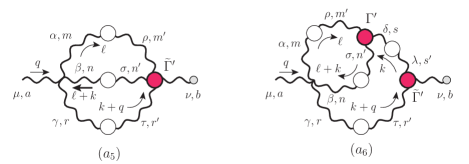
Figure 5: (color online). The two-loop dressed diagrams. The symmetry factors are $1/6$ and $1/2$ respectively.

Before switching on the Schwinger mechanism, the graph $(a_{5})$, for an arbitrary value of the gauge-fixing parameter $\xi$, is given by

$$(a_{5})^{ab}_{\mu\nu}=-\frac{i}{6}{\Gamma}^{(0)amnr}_{\mu\alpha\beta\gamma}\int_{k}\!\int_{\ell}\!\Delta^{\alpha\rho}(\ell)\Delta^{\beta\sigma}(\ell+k)\Delta^{\gamma\tau}(k+q)\widetilde{\Gamma}_{\nu\tau\sigma\rho}^{brnm}(-q,k+q,-\ell-k,\ell),$$ (52)

where the tree-level value of the conventional ($Q^{4}$) four-gluon vertex is given by

$${\Gamma}_{\mu\alpha\beta\gamma}^{(0)amnr} = -ig^{2}[f^{arx}f^{xnm}(g_{\mu\beta}g_{\alpha\gamma}-g_{\mu\alpha}g_{\beta\gamma})+f^{amx}f^{xrn}(g_{\mu\gamma}g_{\alpha\beta}-g_{\mu\beta}g_{\alpha\gamma})$$ (53)

$$+ f^{anx}f^{xrm}(g_{\mu\gamma}g_{\alpha\beta}-g_{\mu\alpha}g_{\beta\gamma})].$$

The fully dressed vertex $BQ^{3}$ satisfies the following WI (all momenta entering)

$$q^{\alpha}\widetilde{\Gamma}^{abcd}_{\alpha\mu\nu\rho}(q,r,p,t) = ig^{2}\left[f^{abx}f^{xcd}\Gamma_{\nu\rho\mu}(p,t,q+r)+f^{acx}f^{xdb}\Gamma_{\rho\mu\nu}(t,r,q+p)\right.$$ (54)

$$+ \left.f^{adx}f^{xbc}\Gamma_{\mu\nu\rho}(r,p,q+t)\right],$$

where it should be emphasized that on the rhs appear the conventional (and not the BFM) trilinear vertices, which satisfy STIs with respect to all their legs, i.e.,

$$q^{\alpha}\Gamma_{\alpha\mu\nu}(q,r,p)=F(q)[p^{2}J(p^{2})P^{\alpha}_{\nu}(p)H_{\alpha\mu}(p,q,r)-r^{2}J(r^{2})P^{\alpha}_{\mu}(r)H_{\alpha\nu}(r,q,p)],$$ (55)

and cyclic permutations Ball and Chiu (1980).

Let us next switch on the Schwinger mechanism. Then, both sides of the WI of Eq. (54) must be replaced by “primed” vertices. Now, the “primed” three-gluon vertices appearing on the rhs are of the type $Q^{3}$, namely $\Gamma^{\prime}_{\alpha\mu\nu}(q,r,p)=\Gamma_{m\alpha\mu\nu}(q,r,p)+{V}_{\alpha\mu\nu}(q,r,p)$, where $\Gamma_{m}$ satisfies Eq. (55) with $J\to J_{m}$ (and $H\to H_{m}$, which, however, we refrain from indicating), while $V$ must satisfy, correspondingly,

$$q^{\alpha}V_{\alpha\mu\nu}(q,r,p)=F(q)[m^{2}(r^{2})P^{\alpha}_{\mu}(r)H_{\alpha\nu}(r,q,p)-m^{2}(p^{2})P^{\alpha}_{\nu}(p)H_{\alpha\mu}(p,q,r)],$$ (56)

and cyclic permutations. Note the difference between Eq. (56) and the corresponding relation satisfied by ${\widetilde{V}}$, given in Eq. (16): the latter is an Abelian WI with no reference to the ghost sector, while the former is an STI, depending explicitly on the ghost-related quantities $F$ and $H$.

Then, the only possibility for maintaining the original WI of Eq. (54) intact is if the quadrilinear vertex on its lhs gets also modified into a vertex satisfying the identity

$$q^{\alpha}\widetilde{\Gamma}^{\prime abcd}_{\alpha\mu\nu\rho}(q,r,p,t) = q^{\alpha}\left[\widetilde{\Gamma}^{abcd}_{{m}\,\alpha\mu\nu\rho}(q,r,p,t)+\widetilde{V}^{abcd}_{\alpha\mu\nu\rho}(q,r,p,t)\right]$$ (57)

$$= ig^{2}\left[f^{abx}f^{xcd}\Gamma^{\prime}_{\nu\rho\mu}(p,t,q+r)+f^{acx}f^{xdb}\Gamma^{\prime}_{\rho\mu\nu}(t,r,q+p)\right.$$

$$+ \left.f^{adx}f^{xbc}\Gamma^{\prime}_{\mu\nu\rho}(r,p,q+t)\right],$$

where $\widetilde{\Gamma}_{m}$ and $\widetilde{V}$ satisfy separately the no-pole ($\Gamma_{m}$) and pole ($V$) part of the trilinear $Q^{3}$ vertex, respectively. In particular, the $\widetilde{V}$ part, which we will be of central importance in what follows, satisfies

$$q^{\alpha}\widetilde{V}^{abcd}_{\alpha\mu\nu\rho}(q,r,p,t) = ig^{2}\left[f^{abx}f^{xcd}V_{\nu\rho\mu}(p,t,q+r)+f^{acx}f^{xdb}V_{\rho\mu\nu}(t,r,q+p)\right.$$ (58)

$$+ \left.f^{adx}f^{xbc}V_{\mu\nu\rho}(r,p,q+t)\right].$$

VI.2 The contribution $a_{5}^{\widetilde{V}}(q^{2})$.

Let us now focus on the part of the diagram $(a_{5})$ that contains the pole component $\widetilde{V}$ of the fully-dressed $BQ^{3}$ vertex $\widetilde{\Gamma}^{\prime}$, to be denoted by $(a_{5}^{\widetilde{V}})$. The projection to the Landau gauge is straightforward, since there are no $\xi^{-1}$ terms anywhere in this diagram, and one obtains

$$(a_{5}^{\widetilde{V}})_{\mu\nu}^{ab}=\frac{i}{6}{\Gamma}_{\mu\alpha\beta\gamma}^{(0)amnr}\int_{k}\int_{\ell}\Delta^{\alpha\rho}(\ell)\Delta^{\beta\sigma}(\ell+k)\Delta^{\gamma\tau}(k+q)\widetilde{V}_{\nu\tau\sigma\rho}^{brnm}(-q,k+q,-\ell-k,\ell),$$ (59)

where all gluon propagators assume the transverse form of Eq. (35).

We can apply the totally longitudinally coupled condition satisfied by $\widetilde{V}_{\lambda\tau\sigma\rho}$,

$$P_{\nu}^{\lambda}(q)P^{\gamma\tau}(k+q)P^{\beta\sigma}(\ell+k)P^{\alpha\rho}(l)\widetilde{V}_{\lambda\tau\sigma\rho}(-q,k+q,-\ell-k,\ell)=0,$$ (60)

to write (59), after splitting $P_{\nu}^{\lambda}(q)$, as follows

$$(a_{5}^{\widetilde{V}})_{\mu\nu}^{ab}=\frac{i}{6}{\Gamma}_{\mu\alpha\beta\gamma}^{(0)amnr}\frac{q_{\nu}}{q^{2}}\int_{k}\int_{\ell}\Delta^{\alpha\rho}(\ell)\Delta^{\beta\sigma}(\ell+k)\Delta^{\gamma\tau}(k+q)q^{\lambda}\widetilde{V}_{\lambda\tau\sigma\rho}^{brnm}(-q,k+q,-\ell-k,\ell).$$ (61)

Using then the WI (54) adapted to the present kinematics, as well as the results

$$f^{brx}f^{xnm}\Gamma^{(0)amnr}_{\mu\alpha\beta\gamma} = i\frac{3}{2}g^{2}C_{A}^{2}\delta^{ab}(g_{\mu\alpha}g_{\beta\gamma}-g_{\mu\beta}g_{\alpha\gamma});$$

$$f^{bnx}f^{xmr}\Gamma^{(0)amnr}_{\mu\alpha\beta\gamma} = i\frac{3}{2}g^{2}C_{A}^{2}\delta^{ab}(g_{\mu\gamma}g_{\alpha\beta}-g_{\mu\alpha}g_{\beta\gamma});$$

$$f^{bmx}f^{xrn}\Gamma^{(0)amnr}_{\mu\alpha\beta\gamma} = i\frac{3}{2}g^{2}C_{A}^{2}\delta^{ab}(g_{\mu\beta}g_{\alpha\gamma}-g_{\mu\gamma}g_{\alpha\beta});$$ (62)

one finds that each one of the terms of the WI gives rise to an integral of the form

$$t_{j}^{\mu}(q)=t_{j}(q^{2})q^{\mu};\quad j=1,2,3$$ (63)

so that Eq. (61) can be written as

$$(a_{5}^{\widetilde{V}})_{\mu\nu}^{ab}=\frac{i}{4}g^{4}C^{2}_{A}\delta^{ab}\frac{q_{\mu}q_{\nu}}{q^{2}}\sum_{j=1}^{3}t_{j}(q^{2}),$$ (64)

with

$$t_{1}(q^{2}) = \frac{1}{q^{2}}(q_{\beta}g_{\alpha\gamma}-q_{\alpha}g_{\beta\gamma})\int_{k}\int_{\ell}\Delta^{\alpha\rho}(\ell)\Delta^{\beta\sigma}(\ell+k)\Delta^{\gamma\tau}(k+q)V_{\sigma\rho\tau}(-\ell-k,\ell,k);$$

$$t_{2}(q^{2}) = \frac{1}{q^{2}}(q_{\alpha}g_{\beta\gamma}-q_{\gamma}g_{\alpha\beta})\int_{k}\int_{\ell}\Delta^{\alpha\rho}(\ell)\Delta^{\beta\sigma}(\ell+k)\Delta^{\gamma\tau}(k+q)V_{\rho\tau\sigma}(\ell,k+q,-q-\ell-k);$$

$$t_{3}(q^{2}) = \frac{1}{q^{2}}(q_{\gamma}g_{\alpha\beta}-q_{\beta}g_{\alpha\gamma})\int_{k}\int_{\ell}\Delta^{\alpha\rho}(\ell)\Delta^{\beta\sigma}(\ell+k)\Delta^{\gamma\tau}(k+q)V_{\tau\sigma\rho}(k+q,-\ell-k,-q+\ell).$$

Now it turns out that, after the appropriate shifts in the momenta, relabeling the Lorentz dummy indices, and applying the Bose symmetry of $V_{\alpha\beta\gamma}$, the three terms are actually equal. Then, using the totally longitudinally coupled condition for the vertex $V$, and the fact that, in the Landau gauge, $k_{\tau}\Delta^{\gamma\tau}(k+q)=-q_{\tau}\Delta^{\gamma\tau}(k+q)$, we get

$$t(q^{2}) = \sum_{j=1}^{3}t_{j}(q^{2})$$

$$= 3\frac{q_{\tau}}{q^{2}}(q_{\alpha}g_{\beta\gamma}-q_{\beta}g_{\alpha\gamma})\int_{k}\Delta^{\gamma\tau}(k+q)\int_{\ell}\Delta^{\alpha\rho}(\ell)\Delta^{\beta\sigma}(\ell+k)\frac{k^{\lambda}}{k^{2}}V_{\sigma\rho\lambda}(-\ell-k,\ell,k).$$

Then, the integral over $\ell$ is a function of $k$ (but not of $q$), and has two free Lorentz indices, $\alpha$ and $\beta$, so that

$$\int_{\ell}\Delta^{\alpha\rho}(\ell)\Delta^{\beta\sigma}(\ell+k)\frac{k^{\lambda}}{k^{2}}V_{\sigma\rho\lambda}(-\ell-k,\ell,k)=A(k^{2})g^{\alpha\beta}+B(k^{2})k^{\alpha}k^{\beta}.$$ (67)

Therefore,

$$t(q^{2})=3\frac{q_{\tau}}{q^{2}}(q_{\alpha}g_{\beta\gamma}-q_{\beta}g_{\alpha\gamma})\int_{k}\Delta^{\gamma\tau}(k+q)\,[A(k^{2})g^{\alpha\beta}+B(k^{2})k^{\alpha}k^{\beta}].$$ (68)

But this term vanishes, regardless of the closed form of $A(k^{2})$ and $B(k^{2})$, because the prefactor is antisymmetric under the exchange $\alpha\leftrightarrow\beta$, whereas the integral is symmetric.

Thus, one finally arrives at the important result

$$a_{5}^{\widetilde{V}}(q^{2})=0,$$ (69)

namely that the graph $(a_{5})$ makes no contribution to the gluon mass equation.

VI.3 The contributions from graph $(a_{6})$

Let us now consider the graph $(a_{6})$, for a general value of the gauge-fixing parameter $\xi$. This graph contains the $BQ^{2}$ and $Q^{3}$ fully-dressed three-gluon vertices, namely $\widetilde{\Gamma}$ and $\Gamma$. We proceed directly to the massive situation, where these two vertices have been replaced by their “primed” counterparts, namely

$$(a_{6})^{ab}_{\mu\nu} = \frac{3}{4}ig^{4}C^{2}_{A}\delta^{ab}\left(g_{\mu\alpha}g_{\beta\gamma}-g_{\mu\beta}g_{\alpha\gamma}\right)\int_{k}\!\Delta^{\gamma\tau}(k+q)\Delta^{\delta\lambda}(k)\widetilde{\Gamma}^{\prime}_{\nu\tau\lambda}(-q,k+q,-k)$$ (70)

$$\times \int_{\ell}\!\Delta^{\alpha\rho}(\ell)\Delta^{\beta\sigma}(\ell+k)\Gamma^{\prime}_{\sigma\rho\delta}(-\ell-k,\ell,k).$$

Evidently, $\widetilde{\Gamma}^{\prime}$ and $\Gamma^{\prime}$ contain the pole parts $\widetilde{V}$ and $V$, respectively, satisfying the general properties mentioned earlier. We will next isolate the terms proportional to $\widetilde{V}$ and $V$, since it is these terms that determine the corresponding contribution of the entire graph $(a_{6})$ to the gluon mass equation. This amounts to writing the product $\widetilde{\Gamma}^{\prime}\Gamma^{\prime}$ as

$$\widetilde{\Gamma}^{\prime}\Gamma^{\prime} = (\widetilde{\Gamma}_{m}+{\widetilde{V}})(\Gamma_{m}+V)$$ (71)

$$= \widetilde{\Gamma}_{m}\Gamma_{m}+{\widetilde{V}}\Gamma_{m}+\widetilde{\Gamma}_{m}V+{\widetilde{V}}V,$$

and considering only the last three terms.

VI.3.1 Vanishing of the terms proportional to $V$

To proceed with the demonstration, note that if we were in the Landau gauge, i.e., if the gluon propagators in Eq. (70) had the fully transverse form of Eq. (35), then $V$ would vanish identically, due to its property of complete longitudinality, given that it is an internal vertex ($Q^{3}$-type). The limit $\xi=0$ may be taken directly in the part of the graph involving the term ${\widetilde{V}}V$, and therefore this term vanishes immediately. As for the combination $\widetilde{\Gamma}_{m}V$, one can take directly the limit $\xi=0$ everywhere, thus making it vanish, except for the term that contains the tree-level part of $\widetilde{\Gamma}_{m}$ that is proportional to $\xi^{-1}$. Specifically, the tree-level part of the $BQ^{2}$ vertex is given by

$$\widetilde{\Gamma}^{(0)}_{\nu\tau\lambda}(-q,k+q,-k)=\Gamma^{(0)}_{\nu\tau\lambda}(-q,k+q,-k)-\xi^{-1}\Gamma^{{\scriptscriptstyle\rm P}}_{\nu\tau\lambda}(-q,k+q,-k),$$ (72)

where the purely longitudinal “pinch part” $\Gamma^{{\scriptscriptstyle\rm P}}$ is given by

$$\Gamma^{{\scriptscriptstyle\rm P}}_{\nu\tau\lambda}(-q,k+q,-k)=-g_{\nu\lambda}(k+q)_{\tau}-g_{\tau\nu}k_{\lambda}.$$ (73)

The contraction of this term with the propagators $\Delta^{\gamma\tau}(k+q)\Delta^{\delta\lambda}(k)$ (with $\xi$ still general) yields

$$\xi^{-1}\Gamma^{{\scriptscriptstyle\rm P}}_{\nu\tau\lambda}(-q,k+q,-k)\Delta^{\gamma\tau}(k+q)\Delta^{\delta\lambda}(k)=\frac{k^{\delta}}{k^{2}}\Delta_{\nu}^{\gamma}(k+q)+\frac{(k+q)^{\gamma}}{(k+q)^{2}}\Delta_{\nu}^{\delta}(k).$$ (74)

In this way, the $\xi^{-1}$ term cancels, making the limit $\xi\to 0$ smooth. So, after setting $\xi=0$, the second term in Eq. (74) vanishes, because $V$ will be contracted by three transverse projectors; on the other hand, the first term survives, since $V$ is contracted only by two. However, as we will see now, this last term finally also vanishes, due to a different reason. Specifically, denoting this contribution by $(a_{6}^{V})_{\mu\nu}$ (thus factoring out the trivial color structure $\delta^{ab}$), we have

$$(a_{6}^{V})_{\mu\nu}=\frac{3}{4}ig^{4}C^{2}_{A}\left(g_{\mu\alpha}g_{\beta\gamma}-g_{\mu\beta}g_{\alpha\gamma}\right)\int_{k}\!\Delta_{\nu}^{\gamma}(k+q)\int_{\ell}\!\Delta^{\alpha\rho}(\ell)\Delta^{\beta\sigma}(\ell+k)\frac{k^{\delta}}{k^{2}}V_{\sigma\rho\delta}(-\ell-k,\ell,k).$$ (75)

Now, the integral $\int_{\ell}$ contains $k$ but no $q$, and has two free Lorentz indices, $\alpha$ and $\beta$; therefore, it can only be proportional to $A(k^{2})g_{\alpha\beta}$ and $B(k^{2})k_{\alpha}k_{\beta}$. But, since both these terms are symmetric under $\alpha\leftrightarrow\beta$, while the prefactor is antisymmetric, this term vanishes.

VI.3.2 The term $a_{6}^{\widetilde{V}}(q^{2})$

Let us finally consider the term ${\widetilde{V}}\Gamma_{m}$ in Eq. (71), to be denoted by $(a_{6}^{\widetilde{V}})_{\mu\nu}$. It is convenient to define the quantity

$$Y_{\delta}^{\alpha\beta}(k)=\int_{\ell}\!\Delta^{\alpha\rho}(\ell)\Delta^{\beta\sigma}(\ell+k)\Gamma_{\sigma\rho\delta}(-\ell-k,\ell,k),$$ (76)

corresponding to the subdiagram on the upper left corner of $(a_{6})$. Then, $(a_{6}^{\widetilde{V}})_{\mu\nu}$ is given by

$$(a_{6}^{\widetilde{V}})_{\mu\nu}=\frac{3}{4}ig^{4}C^{2}_{A}\left(g_{\mu\alpha}g_{\beta\gamma}-g_{\mu\beta}g_{\alpha\gamma}\right)\int_{k}\!Y_{\delta}^{\alpha\beta}(k)\Delta^{\gamma\tau}(k+q)\Delta^{\delta\lambda}(k){\widetilde{V}}_{\nu\tau\lambda}(-q,k+q,-k)$$ (77)

Then, using once again Eqs. (16), (37) and (38), we obtain

$$(a_{6}^{\widetilde{V}})_{\mu\nu} = \frac{3}{4}ig^{4}C^{2}_{A}\left(g_{\mu\alpha}g_{\beta\gamma}-g_{\mu\beta}g_{\alpha\gamma}\right)\frac{q^{\nu}}{q^{2}}\int_{k}\!\left[m^{2}(k)-m^{2}(k+q)\right]\Delta^{\delta}_{\lambda}(k)\Delta^{\gamma\lambda}(k+q)Y_{\delta}^{\alpha\beta}(k)$$ (78)

$$= \frac{q_{\mu}q_{\nu}}{q^{2}}a_{6}^{\widetilde{V}}(q^{2})\,,$$

and so

$$a_{6}^{\widetilde{V}}(q^{2})=\frac{3}{4}ig^{4}C^{2}_{A}\left(q_{\alpha}g_{\beta\gamma}-q_{\beta}g_{\alpha\gamma}\right)\frac{1}{q^{2}}\int_{k}\!\left[m^{2}(k)-m^{2}(k+q)\right]\Delta^{\delta}_{\lambda}(k)\Delta^{\gamma\lambda}(k+q)Y_{\delta}^{\alpha\beta}(k).$$ (79)

At this point it is easy to show that the integral $Y$ is antisymmetric under the $\alpha\leftrightarrow\beta$ exchange; thus, given also the antisymmetry of the $a_{6}^{\widetilde{V}}$ prefactor under the same exchange, one can write

$$Y^{\alpha\beta}_{\delta}(k)=(k^{\alpha}g^{\beta}_{\delta}-k^{\beta}g^{\alpha}_{\delta})Y(k^{2});\qquad Y(k^{2})=\frac{1}{d-1}\frac{1}{k^{2}}\,k_{\alpha}g_{\beta}^{\delta}Y_{\delta}^{\alpha\beta}(k)\,,$$ (80)

which gives us the final result

$$a_{6}^{\widetilde{V}}(q^{2}) = \frac{3}{4}i\frac{g^{4}C^{2}_{A}}{q^{2}}\int_{k}\!m^{2}(k^{2})[(k+q)^{2}-k^{2}][Y(k+q)+Y(k)]\Delta^{\delta}_{\lambda}(k)\Delta_{\delta}^{\lambda}(k+q)$$ (81)

$$+ \frac{3}{4}i\frac{g^{4}C^{2}_{A}}{q^{2}}(q^{2}g_{\delta\gamma}-2q_{\delta}q_{\gamma})\int_{k}\!m^{2}(k^{2})[Y(k+q)-Y(k)]\Delta^{\delta}_{\lambda}(k)\Delta^{\gamma\lambda}(k+q).$$

VI.4 Explicit check of the two-loop dressed blockwise transversality

The vanishing of the term $a_{5}^{\widetilde{V}}$ may appear somewhat surprising, since, in the PT-BFM framework that we employ, it is exactly the $V$ and $\widetilde{V}$ type of vertices that allow for the appearance of a dynamically generated gluon mass in a gauge-invariant way. Thus, one might wonder whether the result (69) is in any way at odds with the characteristic property of the blockwise transversality, mentioned earlier.

To show that this is not the case, let us contract diagram $(a_{5})$ with the physical momentum $q$; after carrying out the usual splitting of the $BQ^{3}$ full vertex $\widetilde{\Gamma}\to\widetilde{\Gamma}_{m}+\widetilde{V}$, using the result (69) and applying the WI (54) to the remaining term, we get

$$q^{\nu}(a_{5}^{\widetilde{\Gamma}^{\prime}})_{\mu\nu}^{ab} = q^{\nu}(a_{5}^{\widetilde{\Gamma}_{m}})_{\mu\nu}^{ab}$$

$$= \frac{3}{4}ig^{4}C_{A}^{2}\delta^{ab}(g_{\mu\beta}g_{\alpha\gamma}-g_{\mu\alpha}g_{\beta\gamma})\int_{k}\!\int_{\ell}\!\Delta^{\alpha}_{\rho}(\ell)\Delta^{\beta}_{\sigma}(\ell+k)\Delta^{\gamma}_{\tau}(k+q)\Gamma_{m}^{\sigma\rho\tau}(-\ell-k,\ell,k).$$

(82)

As far as the contribution of diagram $(a_{6})$ is concerned, we know that it cannot be projected directly to the Landau gauge, because the tree-level part of the fully-dressed $BQ^{2}$ vertex contains terms proportional to $1/\xi$. However, proceeding as in subsection VI.3.1, one writes

$$\widetilde{\Gamma}^{\prime}_{\nu\tau\epsilon}(-q,k+q,-k)=\widetilde{\Gamma}^{\prime\,{\rm reg}}_{\nu\tau\epsilon}(-q,k+q,-k)-\xi^{-1}\Gamma^{\scriptscriptstyle\rm P}_{\nu\tau\epsilon}(-q,k+q,-k),$$ (83)

where evidently the regular part $\widetilde{\Gamma}^{\prime\,{\rm reg}}$ differs from the usual $\widetilde{\Gamma}^{\prime}$ by a tree-level term. For the regular term, after using the identity

$$q^{\nu}\widetilde{\Gamma}^{\prime\,{\rm reg}}_{\nu\tau\epsilon}(-q,k+q,-k)=\Delta^{-1}(k)P_{\tau\epsilon}(k)-\Delta^{-1}(k+q)P_{\tau\epsilon}(k+q),$$ (84)

one gets

$$q^{\nu}(a_{6}^{\widetilde{\Gamma}^{\prime\,{\rm reg}}})_{\mu\nu}^{ab} = \frac{3}{4}ig^{4}C_{A}^{2}\delta^{ab}(g_{\mu\alpha}g_{\beta\gamma}-g_{\mu\beta}g_{\alpha\gamma})\int_{k}\int_{\ell}[\Delta(k+q)-\Delta(k)]P_{\tau\delta}(k)P^{\gamma\tau}(k+q)$$ (85)

$$\times \Delta^{\alpha}_{\rho}(\ell)\Delta^{\beta}_{\sigma}(\ell+k)\Gamma_{m}^{\sigma\rho\delta}(-\ell-k,\ell,k).$$

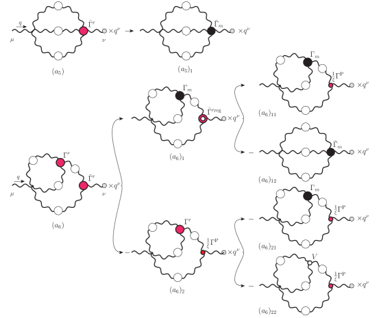
Figure 6: (color online). Diagrammatic realization of the WI for the two-loop dressed diagrams in the Landau gauge. One has the cancellations $(a_{5})_{1}+(a_{6})_{12}=0$ and $(a_{6})_{11}+(a_{6})_{21}=0$, while the term $(a_{6})_{22}$ vanishes.

For the pinch part, after using Eq. (74) to cancel the $\xi^{-1}$ dependence, one obtains (now in the Landau gauge)

$$(a_{6}^{\Gamma^{\scriptscriptstyle\rm P}})_{\mu\nu}^{ab} = \frac{3}{4}ig^{4}C_{A}^{2}\delta^{ab}(g_{\mu\beta}g_{\alpha\gamma}-g_{\mu\alpha}g_{\beta\gamma})\int_{k}\!\left[\frac{k^{\delta}}{k^{2}}\Delta_{\nu}^{\gamma}(k+q)+\frac{(k+q)^{\gamma}}{(k+q)^{2}}\Delta^{\delta}_{\nu}(k)\right]$$ (86)

$$\times \int_{\ell}\!\Delta^{\alpha\rho}(\ell)\Delta^{\beta\sigma}(\ell+k)\Gamma^{\prime}_{\sigma\rho\delta}(-\ell-k,\ell,k).$$

On the other hand, observing that

$$q^{\nu}\bigg{[}\frac{k^{\delta}}{k^{2}}\Delta_{\nu}^{\gamma}(k+q)+\frac{(k+q)^{\gamma}}{(k+q)^{2}}\Delta^{\delta}_{\nu}(k)\bigg{]} = \Delta^{\gamma\delta}(k)-\Delta^{\gamma\delta}(k+q)$$ (87)

$$+ [\Delta(k+q)-\Delta(k)]P^{\delta\nu}(k)P_{\nu}^{\gamma}(k+q),$$

Eq. (86) becomes

$$q^{\nu}(a_{6}^{\Gamma^{P}})_{\mu\nu}^{ab} = \frac{3}{4}ig^{4}C_{A}^{2}\delta^{ab}(g_{\mu\beta}g_{\alpha\gamma}-g_{\mu\alpha}g_{\beta\gamma})\left\{\int_{k}\!\int_{\ell}\!\Delta^{\gamma}_{\delta}(k)\Delta^{\alpha}_{\rho}(\ell)\Delta^{\beta}_{\sigma}(\ell+k)\Gamma_{m}^{\sigma\rho\delta}(-\ell-k,\ell,k)\right.$$

$$- \int_{k}\!\int_{\ell}\!\Delta^{\gamma\delta}(k+q)\Delta^{\alpha\rho}(\ell)\Delta^{\beta\sigma}(\ell+k)\Gamma^{\prime}_{\sigma\rho\delta}(-\ell-k,\ell,k)$$

$$+ \left.\int_{k}\int_{\ell}[\Delta(k+q)-\Delta(k)]P_{\delta}^{\nu}(k)P_{\nu}^{\gamma}(k+q)\Delta^{\alpha}_{\rho}(\ell)\Delta^{\beta}_{\sigma}(\ell+k)\Gamma_{m}^{\sigma\rho\delta}(-\ell-k,\ell,k)\right\}.$$

Clearly the first term integrates to zero, since, being independent of $q$, it cannot saturate its free index $\mu$, while the third term cancels exactly against (85). As far as the second term is concerned, notice that it still contains a pole part, since the total longitudinality condition of Eq. (10) cannot be triggered in this case. However, after splitting the full vertex $\Gamma^{\prime}$ one finds that the $\Gamma_{m}$ part cancels with the term (82), while it is easy to show that the pole part $V$ vanishes along the same lines described when dealing with graph $a_{5}^{\widetilde{V}}$.

The realization of the two-loop dressed blockwise transversality in the Landau gauge is shown diagrammatically in Fig. 6.

VII The full mass equation

After these rather technical considerations, we are now in position to write down the all-order mass equation. Using Eq. (21), together with the results (42) and (81), one finds

$$m^{2}(q^{2}) = \frac{i}{1+G(q^{2})}\left[a_{1}^{\widetilde{V}}(q^{2})+a_{6}^{\widetilde{V}}(q^{2})\right]$$

$$= \frac{ig^{2}C_{A}}{1+G(q^{2})}\frac{1}{q^{2}}\int_{k}m^{2}(k^{2})[(k+q)^{2}-k^{2}]\Delta^{\alpha\rho}(k)\Delta_{\alpha\rho}(k+q)$$

$$\times \left\{1+\frac{3}{4}ig^{2}C_{A}[Y(k+q)+Y(k)]\right\}$$

$$- \frac{3}{4}\frac{g^{4}C_{A}^{2}}{1+G(q^{2})}\frac{1}{q^{2}}(q^{2}g_{\delta\gamma}-2q_{\delta}q_{\gamma})\int_{k}m^{2}(k^{2})[Y(k+q)-Y(k)]\Delta_{\epsilon}^{\delta}(k)\Delta^{\gamma\epsilon}(k+q).$$

The transition to the Euclidean momenta can be performed by using the standard formulas (48) supplemented with the relation $Y_{E}(q^{2}_{E})=-iY(-q_{E}^{2})$; then one obtains (suppressing the “E” subscript as usual)

$$m^{2}(q^{2}) = -\frac{g^{2}C_{A}}{1+G(q^{2})}\frac{1}{q^{2}}\int_{k}m^{2}(k^{2})[(k+q)^{2}-k^{2}]\Delta^{\alpha\rho}(k)\Delta_{\alpha\rho}(k+q)$$

$$\times \left\{1-\frac{3}{4}g^{2}C_{A}[Y(k+q)+Y(k)]\right\}$$

$$+ \frac{3}{4}\frac{g^{4}C_{A}^{2}}{1+G(q^{2})}\frac{1}{q^{2}}(q^{2}g_{\delta\gamma}-2q_{\delta}q_{\gamma})\int_{k}m^{2}(k^{2})[Y(k+q)-Y(k)]\Delta_{\epsilon}^{\delta}(k)\Delta^{\gamma\epsilon}(k+q).$$

Interestingly enough, the full diagrammatic analysis presented in Sections V and VI, in conjunction with the methodology developed in Section IV, may be pictorially summarized, in a rather concise way, as shown in Fig 7.

Note that the quantities entering in Eq. (LABEL:fullmass) are bare, and must eventually undergo renormalization, following the general methodology outlined in various earlier works Aguilar et al. (2009b); Aguilar and Papavassiliou (2010). To be sure, the renormalized version of Eq. (LABEL:fullmass) will involve some of the cutoff-dependent renormalization constants $Z_{i}$ introduced during the renormalization procedure, in a way analogous to what happens in the case of the integral equation for the dynamical quark mass (see, e.g.,  Roberts and Williams (1994); Aguilar and Papavassiliou (2011)); however, for the purposes of the present work, we will ignore these constants (replacing them, effectively, by unity, i.e., $Z_{i}\to 1$ ), and will simply consider Eq. (LABEL:fullmass), assuming that the quantities appearing there are now the renormalized ones.

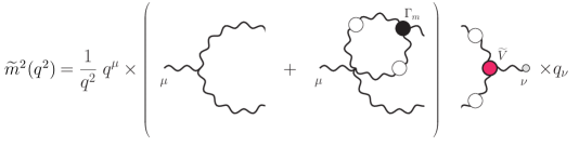
Figure 7: (color online). Diagrammatic representation of the condensed operations leading to the all-order gluon mass equation, where we have introduced the shorthand notation ${\widetilde{m}}^{2}(q^{2})=m^{2}(q^{2})[1+G(q^{2})]$. All internal propagators are in the Landau gauge.

As has been explained in section  IV, the mass equation derived in Eq. (LABEL:fullmass) constitutes one of the two coupled integral equations that govern simultaneously the dynamics of $m^{2}(q^{2})$ and $J(q^{2})$ [see, for example, Eq. (19)]. If the corresponding all order integral equation for $J(q^{2})$ were known, then one could attempt to solve the coupled system, after carrying out the additional substitution $\Delta(k^{2})=[k^{2}J(k^{2})+m^{2}(k^{2})]^{-1}$ [viz. Eq. (12)] to all gluon propagators appearing inside the various kernels. It turns out that the derivation of the all-order integral equation for $J(q^{2})$ is technically far more difficult, mainly due to the presence of the fully dressed four-gluon vertex $BQ^{3}$ [see graph ($a_{5}$) in Fig.2], which is a largely unexplored quantity, with a complicated Lorentz and color structure, and a vast proliferation of form factors. In fact, unlike what happens in the case of the three-gluon vertex $BQ^{2}$ Binosi and Papavassiliou (2011), no gauge-technique Ansatz exists for this four-gluon vertex. Thus, for the rest of this analysis, we will study Eq. (LABEL:fullmass) in isolation, treating all full propagators appearing in it as external quantities, whose form will be determined by resorting to information beyond the SDEs, such as the large-volume lattice simulations. Therefore, Eq. (LABEL:fullmass) is effectively converted into a homogeneous linear integral equation for the unknown function $m^{2}(q^{2})$.

Evidently, the quantity $Y_{\delta}^{\alpha\beta}(k)$ introduced in Eq. (76) accounts for the bulk of the two-loop contribution and depends explicitly on the fully dressed three-gluon vertex $\Gamma$ (of the type $Q^{3}$), in the Landau gauge. This Bose-symmetric vertex satisfies the well-known STI (55) and its cyclic permutations, which allow, in turn, for the reconstruction of the longitudinal form factors of $\Gamma$ in terms of $J$, $F$, and the various form factors of the ghost-gluon kernel $H$ Ball and Chiu (1980). Clearly, the inclusion of the (ten) longitudinal vertex form factors into $Y_{\delta}^{\alpha\beta}(k)$, and through it into Eq. (LABEL:fullmass), will give rise to rather complicated expressions, whose numerical treatment lies beyond the scope of this work.

In what follows we will simplify this preliminary analysis by considering simply the lowest-order perturbative expression for $Y$, obtained by substituting tree-level values for all quantities appearing in Eq. (76), and using (80). It turns out that even so, the resulting expression for $Y$ has sufficient structure to effectively reverse the overall sign of the equation and give rise to physically meaningful solutions for $m^{2}(q^{2})$. In particular, one has

$$Y(k^{2}) = \frac{1}{d-1}\frac{k_{\alpha}}{k^{2}}\int_{\ell}\frac{1}{\ell^{2}(\ell+k)^{2}}P^{\alpha\rho}(\ell)P^{\beta\sigma}(\ell+k)\Gamma^{(0)}_{\sigma\rho\beta}(-\ell-k,\ell,k)$$

$$= \frac{1}{d-1}\frac{k_{\alpha}}{k^{2}}\left(2g_{\beta\sigma}k_{\rho}+g_{\sigma\rho}k_{\beta}-2g_{\beta\rho}k_{\sigma}\right)$$

$$\times \int_{\ell}\frac{1}{\ell^{2}(\ell+k)^{2}}\left[g^{\alpha\rho}g^{\beta\sigma}-\frac{1}{\ell^{2}}(\ell^{\alpha}\ell^{\rho}g^{\beta\sigma}+g^{\alpha\rho}\ell^{\beta}\ell^{\sigma})+\frac{1}{\ell^{2}(\ell+k)^{2}}\ell^{\alpha}\ell^{\rho}(\ell+k)^{\beta}(\ell+k)^{\sigma}\right],$$

and a straightforward calculation yields (in dimensional regularization, Euclidean space)

$$Y(k^{2})=\frac{1}{3(4\pi)^{2}}\left[\frac{15}{4}\left(\frac{2}{\epsilon}\right)-\frac{15}{4}\left(\gamma_{\mathrm{E}}-\log 4\pi+\log\frac{k^{2}}{\mu^{2}}\right)+\frac{63}{12}\right],$$ (92)

where $\mu$ is the ’t Hooft mass introduced at Eq. (6). $Y(k^{2})$ may be renormalized within the MOM scheme, by simply subtracting its value at $k^{2}={\bar{\mu}}^{2}$, yielding

$$Y_{\mathrm{R}}(k^{2})=-\frac{1}{(4\pi)^{2}}\frac{5}{4}\log\frac{k^{2}}{{\bar{\mu}}^{2}}.$$ (93)

VIII Numerical analysis

In this section we carry out a rather thorough numerical analysis of the mass equation derived in the previous sections.

To begin with, let us rewrite the equation (for the $d=4$ case) in a form that will be suited for the ensuing numerical treatment. After setting $x=q^{2}$, observing that $(k+q)^{2}=x+y+2\sqrt{xy}\cos\theta$, and using the measure

$$\int_{k}=\frac{1}{(2\pi)^{3}}\int_{0}^{\pi}\!{\rm d}\theta\,\,\sin^{2}\theta\int_{0}^{\infty}\!{\rm d}y\,\,y,$$ (94)

we obtain

$$m^{2}(x) = -\lambda\frac{F(x)}{x}\int_{0}^{\pi}\!{\rm d}\theta\,\,\sin^{2}\theta\int_{0}^{\infty}\!{\rm d}y\,\,y\,m^{2}(y)\Delta(y)\Delta(x+y+2\sqrt{xy}\cos\theta)$$ (95)

$$\times \left\{A(x,y,\theta)B(x,y,\theta)\left[1-C\left(Y(x+y+2\sqrt{xy}\cos\theta)+Y(y)\right)\right]\right.$$

$$- \left.CE(x,y,\theta)\left(Y(x+y+2\sqrt{xy}\cos\theta)-Y(y)\right)\right\},$$

where we have used the approximation Aguilar et al. (2009b) $1+G(x)\approx F^{-1}(x)$, and set

$$A(x,y,\theta) = 3-\frac{x\sin^{2}\theta}{x+y+2\sqrt{xy}\cos\theta};$$

$$B(x,y,\theta) = x+2\sqrt{xy}\cos\theta;$$

$$E(x,y,\theta) = \frac{xy+x\cos^{2}\theta(x+2\sqrt{xy}\cos\theta)+2(x+\sqrt{xy}\cos\theta)^{2}}{x+y+2\sqrt{xy}\cos\theta}.$$ (96)

and we have defined ($\alpha_{s}=g^{2}/4\pi$)

$$\lambda=\frac{\alpha_{s}C_{A}}{2\pi^{2}},$$ (97)

In addition, we have introduced the constant $C$, multiplying the contribution to the mass equation that is of pure two-loop origin. Of course, the value of $C$ corresponding to the approximate expression Eq. (93) that we employ is fixed, namely

$$C=3\pi C_{A}\alpha_{s};$$ (98)

however, during a significant part of the ensuing analysis we will treat $C$ as a free parameter. Thus, essentially, one disentangles $C$ from the value of $\alpha_{s}$, and studies what happens to the gluon-mass equation when one varies independently $\alpha_{s}$ and $C$. The reason for doing this is twofold: (i ) one has the ability to switch off completely the two-loop corrections (by setting $C=0$), and (ii ) by varying the value of $C$ one may study, in some additional detail, the quantitative impact of the two-loop contribution. Specifically, the philosophy underlying point (ii ) is that, whereas the expression in Eq. (93) furnishes a concrete form for the two-loop correction, by no means does it exhaust it; thus, by varying $C$ we basically model, in a rather heuristic way, further correction that may be added to the “skeleton” provided by the $Y(k^{2})$ of Eq. (93) (for a fixed value of $\alpha_{s}$). Of course, the case where $C$ admits the actual value of Eq. (98) will emerge as a special case of this general two-parameter study. In view of the ensuing analysis it is convenient to measure $C$ in units of $3\pi C_{A}$; to this end, we introduce the reduced parameter $C_{r}=C/3\pi C_{A}$, and drop the suffix “$r$” in what follows.

The integral equation to solve is a homogenous Fredholm equation of the second kind, and can be rewritten schematically as

$$m^{2}(x)=-\lambda\int_{0}^{\pi}\!{\rm d}\theta\,\!\int_{0}^{b}\!{\rm d}y\,\,{\cal K}(x,y,\theta)\,m^{2}(y),$$ (99)

where $b=\infty$, but in practice we will choose $b\gg 1$ but finite. A possible way of solving this equation is to expand the unknown function in terms of a suitable function basis, and subsequently determine the coefficients of this expansion. In particular Press et al. (1992); Bloch (1995, 2003), using the Chebishev polynomials of the first kind $T_{k}$, one can write

$$m^{2}(x)=\frac{c_{0}}{2}+\sum_{k=1}^{n}c_{k}T_{k}(x).$$ (100)

In order to determine the $n+1$ coefficients characterizing the expansion, one discretizes $x\in[0,b]$, choosing the $x_{j}$ values that correspond to the extrema of the $n^{\rm th}$ Chebishev polynomial in that interval, i.e.,

$$x_{j}=\frac{b}{2}\cos\left(\frac{\pi}{n}(n-j)\right)+\frac{b}{2},\qquad j=0,\dots,n.$$ (101)

The problem is then reduced to finding the values of $\lambda$ for which the matrix $A+\lambda B$ is singular, where

$$A_{ij}=\delta T_{i}\left(\frac{2x_{j}-b}{b}\right);\qquad B_{ij}=\delta\int_{0}^{\pi}\!{\rm d}\theta\,\!\int_{0}^{b}\!{\rm d}y\,\,{\cal K}(x_{j},y,\theta)\,T_{i}\left(\frac{2x_{j}-b}{b}\right),$$ (102)

and $\delta=1$, unless $i=0$, in which case it is $1/2$. Specifically one is looking for the smallest positive root $\lambda_{s}$ of the generalized characteristic polynomial of the matrices $A$ and $-B$. Provided that $\lambda_{s}$ exists, one can next determine all the expansion coefficients $c_{k}$ by simply assigning to $c_{0}$ a predetermined value (we choose $c_{0}=1$) and then solving the resulting reduced system; the corresponding value of the coupling constant can then be obtained through Eq. (97). The solution can be finally rescaled by an arbitrary (positive) constant, due to the freedom allowed by the linearity of the equation.

VIII.1 The one-loop dressed case

Let us start our analysis from the one-loop dressed case, which corresponds to setting $C=0$ in Eq. (95). Specifically, notice that, as $x\to 0$, this equation reduces to the following nonlinear constraint

$$m^{2}(0)=-\frac{3\pi}{4}\lambda\,F(0)\int_{0}^{\infty}\!{\rm d}y\,\,m^{2}(y){\cal K}_{\rm 1}(y);\qquad{\cal K}_{\rm 1}(y)=\left[{\cal Z}^{2}(y)\right]^{\prime},$$ (103)

where ${\cal Z}(y)=y\Delta(y)$ is the gluon dressing function. Note that the constraint of Eq. (103) is identical to that derived in Aguilar et al. (2011); remember, however, that the full one-loop equation for arbitrary momenta is different, for the reasons explained in Section V.

As explained in Aguilar et al. (2011), the usefulness of Eq. (103) lies in the fact that, already at this level, one may recognize the difficulty in obtaining physical solutions (i.e., positive definite in the entire momentum range), which can be ultimately traced down to the “wrong” sign in front of the equation. In addition, one may explore the conditions that might finally overcome this difficulty, without having to solve the integral equation in its full complexity. In particular, it is clear from Eq. (103) that, in order to have a possibility of obtaining physically meaningful solutions, the kernel ${\cal K}_{1}$ must display a “sufficiently deep” negative region, which might eventually counterbalance the overall minus sign; indeed, we have verified that it would be immediate to obtain positive-definite (and monotonically decreasing) solutions if we could reverse the overall sign of the equation (or, equivalently, the sign of the kernel). Thus, the existence of a negative region in the kernel is a necessary condition for obtaining physical solutions; a positive-definite kernel, would exclude immediately such a possibility. Of course, as we will see shortly, this condition is far from sufficient.

Specifically, using the lattice data for $\Delta(q^{2})$ corresponding to a $SU(3)$ quenched lattice simulation Bogolubsky et al. (2007), one can explicitly verify whether or not (and exactly how) the necessary condition described above is satisfied. These lattice data are plotted in Fig. 8 (left panel); on the same figure we also plot a fit, whose explicit functional form may be found in various recent articles Aguilar and Papavassiliou (2011); Aguilar et al. (2011, 2010)). On the right panel of Fig. 8 we then show the corresponding one-loop dressed kernel ${\cal K}_{1}$, calculated directly from the lattice data and then also using the aforementioned fit. One clearly observes the zero crossing of the kernel (at $q^{2}\sim 0.8$ GeV²) and the corresponding negative region.

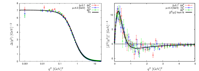
Figure 8: (color online). (Left panel.) Lattice data for the (quenched) $SU(3)$ gluon propagator renormalized at $\mu=4.3$ GeV, shown together with the log fit of Aguilar and Papavassiliou (2011); Aguilar et al. (2011, 2010). (Right panel.) The one-loop dressed kernel derived from the lattice data, compared to the one obtained from the propagator fit.

The propagator fit shown in Fig. 8 can then be used to construct the full kernel appearing in Eq. (95), when $C=0$; the corresponding full integral equation can be then studied by means of the algorithm explained above (for the ghost dressing function $F$, we use a continuous interpolator of the corresponding $SU(3)$ lattice data). It turns out, however, that the solutions obtained have oscillatory behavior, and display large negative regions, ultimately voiding them of any physical meaning.

Evidently, the negative region furnished by the kernel is not sufficiently deep, or it is not located in the optimum momentum region, to counteract the effect of the overall minus sign. Clearly, if physical solutions are to be found, the full functional form of the kernel must be modified. As we will see in the next subsection, this type of appropriate modification is indeed implemented dynamically, when the two-loop corrections are included.

Finally, in order to avoid any confusion related to the conclusions of this subsection and the findings of Aguilar et al. (2011), let us remind the reader that the equation solved in Aguilar et al. (2011) does not coincide with the one solved here; therefore, the (non-monotonic) solutions found in Aguilar et al. (2011), do not correspond to solutions of the present integral equation.

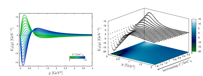
Figure 9: (color online). Modification of the shape of the two-loop dressed kernel ${\cal K}_{2}(y)$ with varying $C$. As the latter parameter increases the kernel effectively reverses its sign showing a deep negative well in the low momenta region.

VIII.2 The two-loop dressed case: finding physical solutions

Let us now turn on again the two-loop dressed contributions, by setting $C>0$. Considering again the $x\to 0$ limit first, one has in this case

$$m^{2}(0)=-\frac{3\pi}{4}\lambda\,F(0)\int_{0}^{\infty}\!{\rm d}y\,m^{2}(y){\cal K}_{\rm 2}(y);\qquad{\cal K}_{\rm 2}(y)=\left\{\left[1-2CY(y)\right]{\cal Z}^{2}(y)\right\}^{\prime}.$$ (104)

Since, as already mentioned, $C$ will be treated as an independent parameter, one can study how the shape of the kernel ${\cal K}_{2}$ changes as $C$ is varied. As can be seen in  Fig. 9, when $C=0$ one is back to the one-loop dressed kernel ${\cal K}_{1}$ of the previous subsection. As $C$ increases ${\cal K}_{2}$ displays a less pronounced positive (respectively negative) peak in the small (respectively large) momenta region. Next, for $C\gtrsim 0.37$, a small negative region starts to appear in the IR, which rapidly becomes a deep negative well for $y\lesssim 0.6$, with ${\cal K}_{2}$ becoming positive for higher momenta. Therefore, we see that the addition of the two-loop dressed contributions counteracts the effect of the overall minus sign of the integral equation, by effectively achieving a sign reversal of the kernel (roughly speaking, one has ${\cal K}_{2}\approx-{\cal K}_{1}$). When this analysis is combined with the knowledge gathered from the one-loop dressed case, one concludes that there exists a critical value $\overline{C}$, such that, if $C>\overline{C}$ Eq. (104) will display at least one physical monotonically decreasing solution for a suitable value of the strong coupling $\alpha_{s}$.

          

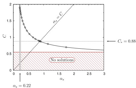
Figure 10: (color online). The curve described by the set of the pairs $(C,\alpha_{s})$ for which one finds physical solutions to the full mass equation (95). The curve starts from the critical value $\overline{C}\approx 0.56$ above which exactly one monotonically decreasing solution exists (below $\overline{C}$ there are no solutions). The value $C_{*}=\alpha_{s}(\approx 0.88)$ corresponds to the case in which $Y$ is kept at its lowest order perturbative value. Finally, the gray vertical band represents the value for the quenched strong coupling obtained from the four-loop MOM calculation of Boucaud et al. (2006) renormalized at $\mu=4.3$ GeV ($\alpha_{s}=0.22$) with a customary $10\%$ error; the matching values of $C$ are between $1.8$ and $1.9$.

In order to see if the picture sketched above is confirmed when $x\neq 0$, one can study numerically the solutions of the full mass equation (95) following the algorithm described at the beginning of the section (Fig. 10). Specifically, as shown in Fig. 10, there is a continuous curve formed by the pairs ($C,\alpha_{s}$), for which one finds physical solutions. Indeed, for small values of $C$ one has that all eigenvalues $\lambda$ are either negative or complex, and no solution exists; this absence of solutions persists until the critical value $\overline{C}\approx 0.56$ is reached, after which one finds exactly one monotonically decreasing solution corresponding to the smallest positive eigenvalue $\lambda_{s}$ (with bigger positive eigenvalues giving rise to oscillating non-physical solutions). However, for values up to $C\approx 0.8$ the coupling needed to get the corresponding running mass is of ${\cal O}(1)$, while for the quenched case the expected coupling from the 4-loop (momentum subtraction) calculation is $\alpha_{s}=0.22$ at $\mu=4.3$ GeV Boucaud et al. (2006). This latter value is obtained for $C\approx 1.8$ – $1.9$, whereas for $C\approx 0.88$ one finds the solution to Eq. (95) for the lowest-order perturbative value of the coefficient (98). In general one observes, as expected, that as $C$ is increased, $\alpha_{s}$ decreases, e.g., for $C=1.1$, $1.3$, $1.5$, and $1.7$ one obtains solutions corresponding to the strong coupling values $\alpha_{s}\approx 0.53$, $0.39$, $0.30$, and $0.25$, respectively.

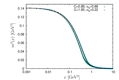
Figure 11: (color online). Typical monotonically decreasing solution of the mass equation (95). The case shown have been obtained for the special values $C=0.88$ and $1.85$, corresponding value of the coupling $\alpha_{s}\approx 0.88$ and $0.22$, respectively. The solutions have been normalized so that at zero they match the corresponding (Landau gauge) lattice value $\Delta^{-1}(0)\approx 0.141$ GeV².

In Fig. 11 we plot the solutions for the most representative $C$ values, i.e., $C=0.88$ and $C=1.85$ (corresponding to, as already said, $\alpha_{s}\approx 0.88$ and $0.22$, respectively); notice that we have used the linearity of the equation to normalize the solution in such a way that the mass at zero coincides with the IR saturating value found in lattice (Landau gauge) quenched simulations Bogolubsky et al. (2009), or $m^{2}(0)=\Delta^{-1}(0)\approx 0.141$ GeV². As can be readily appreciated, the masses obtained display the basic qualitative features expected on general field-theoretic considerations and employed in numerous phenomenological studies; in particular, they are monotonically decreasing functions of the momentum, and vanish rather rapidly in the ultraviolet Cornwall (1982); Lavelle (1991); Aguilar and Papavassiliou (2008). It would seem, therefore, that the all-order analysis presented here, puts the entire concept of the gluon mass, and a variety of fundamental properties ascribed to it, on a solid first-principle basis.

IX Conclusions

In the present work we have derived the full non-perturbative integral equation that governs the momentum evolution of the dynamical gluon mass. This has been accomplished by determining through detailed calculations the mass-related contributions of the “two-loop dressed” graphs that appear in the SDE of the gluon propagator, within the PT-BFM framework. Thus, the complete equation emerges by including these latter contributions to those obtained from the one-loop dressed analysis presented in Aguilar et al. (2011).

We have explained in detail the methodology that allows for a systematic and expeditious identification of the parts of the SDE that contribute to the mass equation. In particular, given the manifest transversality of the full gluon self-energy, we have focused on the $q_{\mu}q_{\nu}$ component of the answer, thus avoiding a number of technical subtleties related to the use of the “seagull identity”. Then, the relevant contributions stem entirely from the parts of the diagrams that involve the special nonperturbative vertices associated with the Schwinger mechanism (generically denoted by $V$), which are longitudinally coupled, contain massless poles, and satisfy relatively simple WIs. In fact, the fully longitudinal nature of these vertices, coupled to the use of the Landau gauge, obviates the need of their explicit construction; indeed, the desired result may be obtained simply by resorting to the WIs that these vertices obey, without the need to invoke their explicit closed form.

It turns out that the inclusion of two-loop dressed contributions has a profound impact on the nature of the mass equation, already at the qualitative level. In fact, the kernel of the integral equation acquires an extra term, with respect to the one-loop case Aguilar et al. (2011), whose presence modifies the nature of the obtained solutions. Specifically, even within the simplest one-loop approximation, this additional term allows for the appearance of positive-definite and monotonically decreasing solutions for the gluon mass $m^{2}(q^{2})$. A detailed numerical investigation of the resulting homogeneous linear integral equation was performed, and the dependence of the solutions on the value of the strong coupling $\alpha_{s}$ and an appropriately introduced parameter $C$ expressing our uncertainty on the two-loop term $Y(k^{2})$, has been studied.

Our analysis reveals that there is a critical $C$ value ($\overline{C}\approx 0.56)$ below which no physically admissible solutions may be found. On the other hand, perfectly acceptable solutions are obtained above this value, with the solution corresponding to the strong coupling $\alpha_{s}=0.22$, predicted at $\mu=4.3$ GeV in the MOM scheme, obtained for $C=1.85$. Within the lowest-order approximation employed for calculating the two-loop dressed term $Y$, a monotonically decreasing mass is obtained for the strong coupling value $\alpha_{s}\approx 0.88$. The fact that already, within this simple approximation for $Y$, one is able to obtain a solution of the full mass equation for a relatively modest size strong coupling should be regarded as a success of the entire PT-BFM framework.

Given the importance of the term $Y(k^{2})$ for this entire construction, it would certainly be important to determine its structure beyond the one-loop approximation used. As already mentioned in Section VII, this can be accomplished, to a certain extent, by making use of the Ball and Chiu Ansatz for the three-gluon vertex Ball and Chiu (1980). An alternative might be lattice itself, given that the three-gluon vertex is (i ) computed in the Landau gauge, and (ii ) it is naturally contracted by three transverse projection operators [see Eqs. (76) and (79)]. Interestingly enough, the resulting structure $PPP\Gamma$ is precisely the one that is accessible to Landau gauge lattice simulations of the gluon three-point function Cucchieri et al. (2008).

The full mass equation, even with the approximate version of $Y(k^{2})$, provides a natural starting point for calculating reliably the effect that the inclusion of light quark flavors might have on the form of the gluon propagator in general, and on the gluon mass in particular. Specifically, recent studies based on SDEs Aguilar et al. (2012b) as well as lattice simulations for $N_{f}=2$, and $N_{f}=2+1+1$ Ayala et al. (2012), appear to converge to the conclusion that the quark effects tend to suppress the gluon propagator in the intermediate and low-momentum region, causing it to saturate at a slightly lower point, compared to the saturation point observed in the quenched case. Should this picture persists further scrutiny, it would seem to indicate, among other things, that the gluon mass increases in the presence of light quarks. It would be, therefore, important to obtain a concrete estimate for the behavior of the gluon mass in the presence of dynamical quarks and especially its value at the origin, i.e., $m^{2}(0)$. We hope to be able to report progress in this direction in the near future.