Network evolution towards optimal dynamical performance

Abstract

Understanding the mutual interdependence between the behavior of dynamical processes on networks and the underlying topologies promises new insight for a large class of empirical networks. We present a generic approach to investigate this relationship which is applicable to a wide class of dynamics, namely to evolve networks using a performance measure based on the whole spectrum of the dynamics’ time evolution operator. As an example, we consider the graph Laplacian describing diffusion processes, and we evolve the network structure such that a given sub-diffusive behavior emerges.

1 Introduction

The importance of networks as a fruitful modeling approach to very diverse scientific areas is nowadays well established. While initially the network topologies were in the focus of investigation, presently the main interest lies in dynamics taking place on networks—in the sense that the network defines the interaction pattern between the individual elements of the dynamical process [1, 2, 3, 4, 5, 6]. Additionally, networks are commonly evolving over time and alter their structure due to random mutations or directed changes, growth, or shrinkage, modifying the dynamical behavior. Since in most cases the functionality of a network is provided by the dynamics, evolution favors structures with a better dynamical performance and eventually adapts towards an optimal topology. A deeper understanding of this mutual relation between structure and dynamics can be achieved either by studying empirical systems directly, in a biological context for instance physiological networks [7], food webs [8], or protein interaction networks [9], or by modeling of network evolution towards a desired dynamical performance and in this way gain new insight into many empirical networks. Concerning the latter, the evolution of dynamical networks was previously applied in the contexts of modularity in changing environments [10], Boolean (threshold) dynamics [11, 12, 13, 14, 15, 16], and synchronization of oscillatory systems [17, 18, 19, 20, 21]. It is known that the dynamical behavior is closely related to the network’s spectral properties [22], which was exploited in studies in which the Laplacian eigenratio [23] was maximized by network evolution [17, 18, 19, 20]. Other studies carried out the dynamics explicitly [11, 12, 13, 14, 15, 21], which can be computationally very costly.

In this Letter, we present an alternative approach based on the whole eigenvalue spectrum of the time evolution operator $\mathcal{O}_{\mathbf{A}}$ of linear dynamics. Specifically, we consider dynamics on a network with $N$ vertices described by a linear equation,

$$\frac{\mathrm{d}\mathbf{p}(t)}{\mathrm{d}t}=\mathcal{O}_{\mathbf{A}}\,\mathbf{p}(t)\,,$$ (1)

where $\mathbf{p}(t)=(p_{1}(t),\ldots,p_{N}(t))^{\mathrm{T}}$ represents the dynamical state at time $t$. Depending on the problem under consideration, $\mathbf{p}(t)$ can denote the activity of the individual vertices, their phases, the distribution of a substance flowing across the network, the probability distribution of some event to occur, etc. The operator $\mathcal{O}_{\mathbf{A}}$ depends on the network topology described by the $N\times N$ adjacency matrix $\mathbf{A}$ of the network (with elements $A_{ij}=1$ if vertex $i$ is linked to vertex $j$ and $A_{ij}=0$ otherwise). In contrast to studies on coevolutionary networks [24], we regard the time scales of the dynamics on the network and of the structure modifications as being well separated, which is the case in many empirical networks (consider for example cellular processes such as protein-protein interaction or gene regulation compared to biological evolution).

2 Model

The eigenvalues of $\mathcal{O}_{\mathbf{A}}$, $\lambda_{\nu}$, can be represented in a functional form by the integrated density of states (DOS),

$$I(\lambda)=\frac{1}{N}\,\sum_{\nu=1}^{N}\Theta(\lambda-\lambda_{\nu})\,,$$ (2)

where $\Theta$ denotes the Heaviside step function, $\Theta(x)=1$ for $x\geq 0$ and $\Theta(x)=0$ for $x<0$. Our approach to quantify the dynamical performance via the eigenvalue spectrum is to establish a distance metric $\Delta(I,I^{\mathrm{target}})$ between any $I$ and a predefined (but not necessarily realizable) $I^{\mathrm{target}}$ yielding the desired dynamical behavior. The evolution of a network structure consists of two parts, carried out in each evolution step $n$. First, a candidate network is constructed from the present one by a random modification in the topology (mutation). Secondly, the candidate is accepted or rejected for the next step by a criterion based on the values of $\Delta(I,I^{\mathrm{target}})$ before and after the mutation (selection). If the distance metric and the criteria for mutation and selection are chosen appropriately, the evolution will eventually converge to an optimal network structure for a given $\mathcal{O}_{\mathbf{A}}$ and desired dynamical behavior.

In the following discussion, we exemplify our approach by considering simple graphs and the graph Laplacian $\mathbf{L}$, given by

$$L_{ij}=\delta_{ij}k_{i}-A_{ij}=\begin{cases}k_{i}&\textrm{if }i=j\,,\\ -A_{ij}&\textrm{if }i\neq j\,,\end{cases}$$ (3)

with $\delta_{ij}$ being Kronecker’s delta and $k_{i}\equiv\sum_{j}A_{ij}$ the degree of vertex $i$, as dynamical operator, i.e., $\mathcal{O}_{\mathbf{A}}=-C\mathbf{L}$ with $C>0$ being a (diffusion) constant. The graph Laplacian $\mathbf{L}$ is of importance in many physical situations [25], such as electrical or other flow networks [26], Gaussian spring networks as polymer models [27], random walks [28] as the space discrete equivalent of diffusion, and synchronization [29]. In the context of diffusion, $\mathbf{p}(t)$ denotes the probability to find the random walker at a given vertex at time $t$ and eq. (1) is the master equation describing its time evolution. Many properties of the random walk, such as the average probability of returning to the origin at time $t$, $P_{0}(t)=N^{-1}\sum_{i=1}^{N}\exp(-\lambda_{\nu}\,t)$, are determined by the spectral dimension $d_{\mathrm{s}}$ defined via the scaling of the integrated DOS [30],

$$I(\lambda)\propto\lambda^{d_{\mathrm{s}}/2}\,.$$ (4)

It is known that $P_{0}(t)$ decays for $t\to\infty$ as a power-law, $P_{0}(t)\propto t^{-d_{\mathrm{s}}/2}$ [31]. For all uniform Euclidean systems without broad waiting time distributions, the mean-square displacement of the random walk scales linear with $t$ and $P_{0}(t)$ decays as $t^{-d/2}$ where $d$ is the spatial dimension. This behavior is called normal diffusion and the corresponding spectral dimension is $d_{\mathrm{s}}^{\mathrm{(n)}}=d$, whereas non-linear scaling is referred to as anomalous diffusion [30]. An interesting and challenging goal is to optimize a network structure for a given fixed $1<d_{\mathrm{s}}<2$, such that $P_{0}(t)$ decays slower than in the regular two-dimensional (2d) case (sub-diffusion), which will be the desired dynamical behavior in the following.

In the present case of the graph Laplacian, there are two issues to be addressed. First, the scale of the Laplacian eigenvalues is to first order given by the degrees $\{k_{i}\}$ as largest elements of $\mathbf{L}$, located along the diagonal, whereas all non-zero off-diagonal elements are $-1$. Hence, we consider the rescaled eigenvalues $\tilde{\lambda}_{\nu}=\lambda_{\nu}/\max_{\nu^{\prime}}\{\lambda_{\nu^{\prime}}\}$, which reduces the dependence of the eigenvalue spectrum on the degrees and does not change the scaling of $I(\lambda)$. Second, since the spectral dimension $d_{\mathrm{s}}$ appears in the exponent of eq. (4), we introduce the logarithmically integrated DOS,

$$\tilde{I}(\ln\tilde{\lambda})=\ln\left(\frac{1}{N}\,\sum_{\nu=1}^{N}\Theta(\ln\tilde{\lambda}-\ln\tilde{\lambda}_{\nu})\right)\,.$$ (5)

The measure of dynamical performance can then be defined by the metric

$$\Delta(\tilde{I},\tilde{I}^{\textrm{target}})=\int_{\ln\tilde{\lambda}_{\mathrm{min}}}^{0}\,\left|\tilde{I}(\ln\tilde{\lambda})-\tilde{I}^{\textrm{target}}(\ln\tilde{\lambda})\right|^{2}\,\mathrm{d}\ln\tilde{\lambda}$$ (6)

where $\tilde{I}$ is the present and $\tilde{I}^{\textrm{target}}$ is the target logarithmically integrated DOS. The lower integration boundary $\ln\tilde{\lambda}_{\mathrm{min}}$ is chosen such that $\tilde{I}^{\textrm{target}}(\ln\tilde{\lambda})<\ln(N^{-1})$ for $\ln\tilde{\lambda}<\ln\tilde{\lambda}_{\mathrm{min}}$ and $\tilde{I}^{\textrm{target}}(\ln\tilde{\lambda})\geq\ln(N^{-1})$ for $\ln\tilde{\lambda}\geq\ln\tilde{\lambda}_{\mathrm{min}}$. (Note that $\tilde{I}^{\textrm{target}}(\ln\tilde{\lambda})$ is a monotonic, but not necessarily continuous function; if $\tilde{I}^{\textrm{target}}(\ln\tilde{\lambda})$ is continuous, then $\tilde{I}^{\textrm{target}}(\ln\tilde{\lambda}_{\mathrm{min}})=\ln(N^{-1})$.)

Concerning the basic evolution step, we have chosen the mutation such that a minimal change in the eigenvalue spectrum is ensured. A randomly chosen edge is removed from the network and a new edge between two previously unconnected vertices is introduced. The selection consist of two parts. If the modification separates the network into two disconnected components then it is rejected directly. Otherwise, the mutation is accepted if it decreases the value of the metric $\Delta(\tilde{I},\tilde{I}^{\textrm{target}})$. In this way, the evolving network performs an adaptive walk in the space of connected simple graphs with both numbers of vertices $N$ and edges $M$ fixed.

3 Results

As a first test of our evolutionary algorithm, we specify the target integrated DOS as $I^{\textrm{target}}(\lambda)\propto\lambda^{d_{\mathrm{s}}/2}$ yielding $\tilde{I}^{\textrm{target}}(\ln\tilde{\lambda})=d_{\mathrm{s}}/2\,\ln\tilde{\lambda}$, with two exemplary values $d_{\mathrm{s}}^{(1)}=1.4$ and $d_{\mathrm{s}}^{(2)}=1.1$ both in the sub-diffusive regime well below $d_{\mathrm{s}}^{\mathrm{(n)}}=2$ for a two-dimensional system. In order to verify to which extent the outcome of the evolution depends on the initial conditions, i.e., how much of the evolutionary history remains imprinted in the networks, we start the evolution from two classes of initial networks, (i) 2d square lattices with periodic boundary conditions; and (ii) connected random graphs $G(N,M)$ (simple graphs with $N$ vertices and $M$ randomly chosen edges, restricted to form a single connected component). While in 2d square lattices all vertices have the same degree $k=4$, random graphs $G(N,M)$, just as the famous Erdős-Rényi networks, obey a Poisson degree distribution, $P(k)=\eta^{k}\mathrm{e}^{-\eta}/k!$, with mean degree $\langle k\rangle\equiv\eta=4$ here. All inital networks are chosen to have $N=361$ vertices. Each evolution is driven for $10^{6}$ steps and repeated with different random seeds for $100$ realizations.

Figure 1: (Color online) Distribution of the distance measures $\Delta(\tilde{I},\tilde{I}^{\textrm{target}})$ as a function of the step number $n$ evolving with a power-law DOS $\tilde{I}^{\textrm{target}}(\ln\tilde{\lambda})=d_{\mathrm{s}}/2\,\ln\tilde{\lambda}$ with $d_{\mathrm{s}}^{(1)}=1.4$ (main plot) and $d_{\mathrm{s}}^{(2)}=1.1$ (inset) as target. The lines display the mean distance measure of $100$ realizations of the evolution starting from 2d square lattices (green dashed lines) and random graphs (red solid lines), and the error bars mark one standard deviation of the respective distributions.

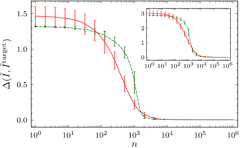
In fig. 1, the distributions of the distance measure $\Delta(\tilde{I},\tilde{I}^{\textrm{target}})$ are shown as a function of the step number $n$ for the evolution starting with networks from the two classes of initial networks and evolving towards $d_{\mathrm{s}}^{(1)}=1.4$ (main plot) and $d_{\mathrm{s}}^{(2)}=1.1$ (inset). In all cases, the distance measure $\Delta(\tilde{I},\tilde{I}^{\textrm{target}})$ decreases slowly for about $10^{2}$ steps, then drops quickly by an order of magnitude within the following decade, and afterwards continues to decrease only marginally. The distributions of the distance measure $\Delta(\tilde{I},\tilde{I}^{\textrm{target}})$ for the two choices of initial conditions become indistinguishable after around $10^{4}$ evolution steps.

Figure 2: (Color online) Logarithmically integrated DOS $\tilde{I}(\ln\tilde{\lambda})$ exemplified using individual realizations, two initial networks (light colors) and two networks after $10^{6}$ evolution steps with different $\tilde{I}^{\textrm{target}}(\ln\tilde{\lambda})$ (dark colors). Results are shown for evolutions with $d_{\mathrm{s}}^{(1)}=1.4$ starting from a 2d square lattice (green dashed lines) and $d_{\mathrm{s}}^{(2)}=1.1$ starting from a random graph (red solid lines). The two target logarithmically integrated DOS $\tilde{I}^{\textrm{target}}(\ln\tilde{\lambda})=d_{\mathrm{s}}/2\,\ln\tilde{\lambda}$ are shown as references (black dotted lines) with annotated slopes.

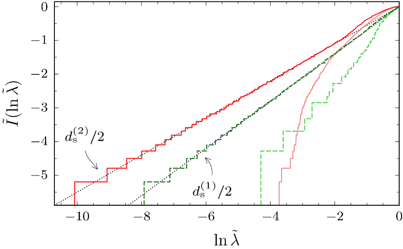
Typical realizations of the logarithmically integrated DOS, as occurring during the evolution process shown in fig. 1, are depicted in fig. 2. We display four examples, two initial networks and two networks at step $n=10^{6}$, having been evolved with target $d_{\mathrm{s}}^{(1)}=1.4$ from an initial 2d square lattice with periodic boundary conditions and $d_{\mathrm{s}}^{(2)}=1.1$ from a connected random graph $G(N,M)$. One notices that after $10^{6}$ steps, the logarithmically integrated DOS follows the respective target, $\tilde{I}^{\textrm{target}}(\ln\tilde{\lambda})=d_{\mathrm{s}}/2\,\ln\tilde{\lambda}$, very closely up to immanent discretization.

Figure 3: (Color online) Average probability $P_{0}(t)$ for a random walker to return to its origin at time $t$ on the initial networks (light colors) and evolved networks after $10^{6}$ steps with power-law DOS $\tilde{I}^{\textrm{target}}(\ln\tilde{\lambda})=d_{\mathrm{s}}/2\,\ln\tilde{\lambda}$ as targets (dark colors) for evolutions with $d_{\mathrm{s}}^{(1)}=1.4$ starting from 2d square lattices (green dashed lines) and $d_{\mathrm{s}}^{(2)}=1.1$ starting from random graphs (red solid lines). The lines display the mean of $100$ realizations and the error bars mark one standard deviation of the distributions. The black dotted lines are guides to the eye and have slopes of $-d_{\mathrm{s}}^{\mathrm{(n)}}/2=-1$, $-d_{\mathrm{s}}^{(1)}/2=-0.7$, and $-d_{\mathrm{s}}^{(2)}/2=-0.55$, as annotated, indicating the expected scaling behavior.

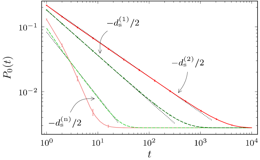
The average probability $P_{0}(t)$ for a random walker to return to its origin at time $t$ is obtained for the initial as well as for the evolved networks and is shown in fig. 3. For the evolved networks, $P_{0}(t)$ indeed follows a power-law $P_{0}(t)\propto t^{-d_{\mathrm{s}}/2}$ with $d_{\mathrm{s}}^{(1)}=1.4$ and $d_{\mathrm{s}}^{(2)}=1.1$, respectively, as expected from the linear scaling of $\tilde{I}(\ln\tilde{\lambda})$ in fig. 2. Note the rather small dynamical heterogeneity indicated by the error bars (displaying one standard deviation).

Figure 4: (Color online)Degree distributions $P(k)$ of—from left to right—the two initial and the corresponding evolved networks after $10^{6}$ evolution steps, i.e., 2d square lattices (1st bar, light green), random graphs with mean $\langle k\rangle=4$ (2nd bar, light red), and the resulting networks after evolution towards a power-law DOS $\tilde{I}^{\textrm{target}}(\ln\tilde{\lambda})=d_{\mathrm{s}}/2\,\ln\tilde{\lambda}$ with $d_{\mathrm{s}}^{(1)}=1.4$ as target (3rd bar, dark green, and 4th bar, dark red). The histogram bars display the mean of $100$ networks, and the error bars mark one standard deviation. The insets display the distribution of Newman coefficients $r$ and clustering coefficients $c$ as a function of the step number $n$ for evolutions starting from 2d square lattices (green dashed lines) and random graphs (red solid lines). The lines display the averages over $100$ networks, and the error bars mark one standard deviation of the distributions.

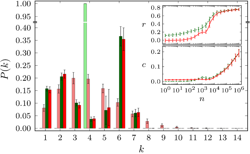
Given the convergence of the dynamical performance, the question arises as to how similar the underlying networks are topologically. In fig. 4, the degree distributions $P(k)$, being the probability that a randomly chosen vertex has degree $k$, of the two initial and the corresponding evolved networks are shown. Despite the dissimilarities in the degree distributions of the two classes of initial networks (Poisson vs. delta distribution), the degree distributions of the evolved networks are quite alike on the level of averages. Nevertheless, there is significant variation from network to network as can be seen, for example, by the large standard deviation for $k=5$ indicated by the error bars. While very few vertices with the average degree $k=4$ are present, the fraction of vertices with higher ($k=6$) and lower ($k=1,2$) degrees increases in the course of the evolution suggesting that the networks become more heterogeneous.

To gain further insight into the resulting network topologies, we display in the insets of fig. 4 the average degree assortativity or Newman coefficient $r$ and the average clustering coefficient $c$ as function of the evolution step number $n$. The Newman coefficient $r$ [32] is the Pearson correlation coefficient of degrees of two vertices connected by an edge and hence measures the amount of degree-degree correlation (degree assortativity) in a network. A network without degree-degree correlations has $r=0$. In our example, the networks become assortative in the course of the evolution ($r>0$), meaning that connections preferentially exist between vertices of similar degree, another indicator for heterogeneity in the network structure. The clustering coefficient $c$, defined as the density of triangles [33], measures the transitivity of a network, i.e., the tendency that the neighbors of a given vertex are connected to one another. For a connected graph with fixed numbers of vertices and edges, an increasing clustering coefficient $c$ indicates, again, a trend towards more heterogeneous structures. We observe that although the network evolution converged in less than $10^{6}$ evolution steps with respect to the dynamical behavior and the Newman coefficient, the clustering coefficient is still increasing and broadly distributed. As the changes in the different observables do not coincide with the changes in the dynamical behavior, we conclude that even with a given eigenvalue spectrum there is some structural freedom left for variation in 3-point properties such as transitivity and, despite the dynamical behavior being essentially identical after $10^{6}$ evolution steps, the underlying network topologies can still be rather diverse. We do not observe any systematic differences between networks evolved from regular lattices or random graphs suggesting that already this simplest version of our evolutionary algorithm suffices to explore the relevant region of the network configuration space in a reasonable number of evolution steps.

4 Conclusion

Most networks, in particular as occurring in biology, are not static entities but instead constantly evolve over time. Even though a given change usually affects the network structure in the first place, its fate is decided by the resulting alteration of the dynamics on the network providing its functionality, so that evolution favors topologies with a better dynamical performance. We study the relationship between network structure and dynamics by means of network evolution using a performance measure based on the whole eigenvalue spectrum of the time evolution operator of linear dynamics. By this, we avoid the explicit calculation of the dynamical time evolution, which can be computationally very costly. To exemplify our approach, we use the graph Laplacian describing a diffusion process, and evolve networks such that a given sub-diffusive behavior emerges. Interestingly, the resulting networks show an overall trend towards heterogeneous structures and, despite displaying essentially the same dynamical behavior, are structurally quite diverse.

5 Acknowledgment

We gratefully acknowledge helpful discussions with Sebastian Weber in early stages of this work and funding by the Studienstiftung des deutschen Volkes and the Bonn-Cologne Graduate School of Physics and Astronomy (SK) and by the Deutsche Forschungsgemeinschaft via the Heisenberg program (PO 1025/6) (MP).