A gas-kinetic scheme for the simulation of turbulent flows

Abstract

Numerical schemes derived from gas-kinetic theory can be applied to simulations in the hydrodynamics limit, in laminar and also turbulent regimes. In the latter case, the underlying Boltzmann equation describes a distribution of eddies, in line with the concept of eddy viscosity developed by Lord Kelvin and Osborne Reynolds at the end of the nineteenth century. These schemes are physically more consistent than schemes derived from the Navier-Stokes equations, which invariably assume infinite collisions between gas particles (or interactions between eddies) in the calculation of advective fluxes. In fact, in continuum regime too, the local Knudsen number can exceed the value $0.001$ in shock layers, where gas-kinetic schemes outperform Navier-Stokes schemes, as is well known.

Simulation of turbulent flows benefit from the application of gas-kinetic schemes, as the turbulent Knudsen number (the ratio between the eddies’ mean free path and the mean flow scale) can locally reach values well in excess of $0.001$, not only in shock layers. A further advantage of gas-kinetic schemes is that the fluxes are accurate to $\tau^{2}$, for instance in the scheme developed in [19] for the finite-volume discretization. In laminar flow, this provides a better resolution of shocks and vortexes, whereas in turbulent flows, high-order fluxes allow for a better resolution of secondary flows in a manner comparable to higher-order turbulence models for the Navier-Stokes schemes.

This study has investigated a few cases of shock - boundary layer interaction comparing a gas-kinetic scheme and a Navier-Stokes one, both with a standard $k-\omega$ turbulence model. Whereas the results obtained from the Navier-Stokes scheme are affected by the limitations of eddy viscosity two-equation models, the gas-kinetic scheme has performed much better without making any further assumption on the turbulent structures.

1 Introduction

Numerical schemes based on the Navier-Stokes (NS) equations have benefited for many years from the valuable work of mathematicians and engineers. Aerodynamicists dispose of accurate and fast simulation tools, which can be applied to complex geometries and challenging flow conditions, providing physically consistent results in many cases.

However, limitations still apply and appear difficult to overcome. They concern the numerical model – dependency of the results on numerical scheme and mesh, steeply increasing computational cost with the order of the scheme, reduction of accuracy at discontinuities – or the physical model – modelling the effect of unresolved turbulence on resolved flow in conditions far from local turbulent equilibrium, simulation of rarefied flow. The prediction of turbulent, hypersonic flow is a particularly challenging example.

Numerical schemes based on gas-kinetic theory, or Gas-Kinetic Schemes (GKS), might help in overcoming these limitations. Firstly, because the Boltzmann equation is a physically more accurate representation of fluid mechanics than the Navier-Stokes equations and secondly, because gas-kinetic can deal much better with the discontinuities that invariably at cells interface in most numerical approaches, since Godunov scheme ([7]).

Navier-stokes schemes split transport and collisions, i.e. advective and viscous fluxes. As such, advective fluxes are generated by the solution of the Riemann problem which does not consider the effect of particle collision. The effect of collisions is added a posteriori by the viscous fluxes, calculated independently. As long as the molecular relaxation time is much smaller than the mean time scale, superposition of fluxes does not affect the physical consistence. However, wherever this assumption is not true, as in the case of shock layers or of rarefied flows, the physical consistence of Navier-Stokes schemes becomes questionable. Despite the fact that Navier-Stokes schemes can predict shocks satisfactorily for many industrial applications, the prediction treats the shock merely as a discontinuity. Moreover, special treatment is often necessary to maintain the stability of the solution in presence of shocks - and this contributes to the dependence of the solution from the chosen method.

The modelling of turbulence can also benefit from the use of GKS. It is recognized since the publications of Lord Kelvin and Osborne Reynolds’ works on turbulence, (refer to [3, 4] and references therein) that the Boltzmann equation, also in the simpler form of the BGK model, can be used to describe not only the flow as distribution of particles but also the turbulent flow as distribution of eddies. Moreover, it is also recognized ([4]) that the projection onto the physical space $(\bf x,t)$ of the BGK model generates a higher-order (in $\tau_{t}$) turbulent stress tensor. In particular a third order Chapman-Enskog expansion for $f$ generates a turbulent stress tensor of the second order, i.e. comparable to non-linear turbulent stress models. These models are known to provide more accurate values than linear models ([13, 17]).

This study focuses on the GKS developed by Xu ([19]) which has also been investigated by other researchers ([12, 16]) and has provided very good results in a number of cases, ranging from viscous-dominated, subsonic flows to hypersonics. It provides fluxes accurate to $\tau^{2}$ and, consequently, a second-order turbulent stress tensor.

This GKS has been implemented into an existing solver which uses a standard $k-\omega$ ([18]) turbulence model. The flow cases investigated are popular aerodynamic benchmarks - all in the continuum regime - characterised by strong shock - boundary layer interaction - that is a flow condition where most two-equation turbulence models fail to predict shock position and extension of separated flow accurately. The equation for the turbulent quantities $k$ and $\omega$ are advanced in a segregate way.

This paper presents a brief description of the GKS for laminar and turbulent flow, followed by the numerical experiments and conclusions.

2 Gas-kinetic scheme

A few gas-kinetic schemes for the solution of the Euler and the Navier-Stokes equations have been proposed in the 1990s ([19, 12, 11, 5, 21] and references therein) as an alternative to the most popular schemes, which normally assume continuity of the flow or solve a Riemann problem at cells interfaces.

The main idea behind these schemes is to consider a discontinuous state across interfaces, re-construct the equilibrium and non-equilibrium distribution functions based on the macroscopic flow variables and calculate the evolution of the distribution functions during a time step $\Delta t$ integrating the BGK-Boltzmann equation. The macroscopic flow quantities are then recovered taking moments of the solution distribution function.

We use the macroscopic variables $\rho$, $U=[u_{1}\,\,\,u_{2}\,\,\,u_{3}]^{T}$, and $E$ to describe density, velocity and total energy of a gas. Instead of using the well-known Navier-Stokes equations, we write the BGK model following [1]:

$$\frac{\partial f}{\partial t}+u_{i}\frac{\partial f}{\partial x_{i}}={(g-f)\over\tau}$$ (1)

where the summation convention holds, $f$ is the gas distribution function, $g$ is the equilibrium state, a Maxwellian distribution, approached by $f$ and $\tau$ is the particles collision time, which is related to the molecular viscosity and heath coefficients of the gas. Although not explicitly indicated, it is assumed in [19] that the collision time can also include the effects of turbulence, beside those of molecular viscosity and numerical dissipation. The variable $\xi$ is related to the additional degrees of freedom of the gas molecules. $\xi$ has $K$ degrees of freedom, where:

$$K=\frac{5-3\gamma}{\gamma-1}+1$$ (2)

where $\gamma$ is the specific heat ratio. The equilibrium distribution is:

$$g=\rho\left(\frac{\lambda}{\pi}\right)^{\frac{K+2}{K}}e^{-\lambda\left((u_{i}-U_{i})^{2}+\xi^{2}\right)}$$ (3)

where $\lambda=\frac{m}{2kT}$, $m$ is the molecular mass, $k$ is the Boltzmann constant, and $T$ is temperature. The relation between macroscopic variables and gas distribution function is:

$$\left\{\begin{array}[]{c}\rho\\ \rho U\\ \rho E\\ \end{array}\right\}=\int\psi fd\Xi$$ (4)

where $\psi$ is:

$$\psi=\left\{\begin{array}[]{c}1\\ U\\ {1\over 2}\left({u_{i}}^{2}+\xi^{2}\right)\end{array}\right\}$$ (5)

note that $d\Xi=du_{1}\,du_{2}\,du_{3}\,\xi^{K-1}\,d\xi$. Conservation of mass, momentum and energy during particle collision is expressed by:

$$\int\left(g-f\right)\psi d\Xi=0$$ (6)

The BGK equation 1 has an analytical solution:

$$f(x,y,z,t,u,v,w,\xi)={1\over\tau}\int_{o}^{t}g(x^{\prime},y^{\prime},z^{\prime},t,u,v,w,\xi)e^{-(t-t^{\prime})/\tau}\,dt^{\prime}+e^{-t/\tau}f_{0}(x-ut,y-vt,z-wt)$$ (7)

where $f_{0}$ is the initial gas distribution function, $x^{\prime}=x-u(t-t^{\prime}),\,\,\,y^{\prime}=y-v(t-t^{\prime}),\,\,\,z^{\prime}=z-w(t-t^{\prime})$. The kernel of the GKS consists in expressing the distribution function $f$ at cells or volumes interfaces in order to assess the fluxes as functions of $f$. For instance the flux in direction $i$ at the interface between cells $n$ and $n+1$ can be expressed as a first moment of $f$:

$$F_{i}^{n+1/2}=\int_{0}^{\Delta_{t}}\int u_{i}^{n+1/2}\,\psi^{n+1/2}\,f(x^{n+1/2})\,d\Xi\,dt$$ (8)

The distribution functions $f_{0}$ and $g$ in the 7 must be consistent with the macroscopic variables and their gradients. An important assumption in the derivation of the GKS is that whereas equilibrium distributions are Maxwellians, the non-equilibrium distribution are expressed as Taylor expansion of Maxwellian distribution. Assuming an interface normal to direction $1$ located at $x_{1}=0$, the initial equilibrium distribution is expressed as:

$$g=\left\{\begin{array}[]{l}g_{0}\left(1+\bar{a}_{i}^{l}x_{i}-\bar{A}t\right),\,\,\,x_{1}<0\\ g_{0}\left(1+\bar{a}_{i}^{r}x_{i}-\bar{A}t\right),\,\,\,x_{1}>0\end{array}\right.$$ (9)

where $g_{0}$ is a Maxwellian derived from a state $\left[\rho_{0}\,\,\,\rho{U_{0}}_{i}\,\,\,\rho_{0}E_{0}\right]$, which is an average state between left and right, obtained in a non-trivial averaging process, which fulfils the BGK model and the conservation laws ([19]). The initial distribution $f_{0}$ can be expressed as:

$$f_{0}=\left\{\begin{array}[]{l}g^{l}(1+a_{i}^{l}x_{i})-\tau\left(a_{i}^{l}u_{i}+A^{l}\right),\,\,\,x_{1}<0\\ g^{r}(1+a_{i}^{r}x_{i})-\tau\left(a_{i}^{r}u_{i}+A^{r}\right),\,\,\,x_{1}>0\end{array}\right.$$ (10)

where $g^{l}$ and $g^{r}$ are Maxwellian distribution on both sides of the interface, which are indicated as left and right. The choice of the terms used in the expansion 10 is critical for the type of GKS. The terms proportional to $\tau$ represent the non-equilibrium parts in the Chapman-Enskog expansion ([2]), whereas the expansion in the spatial directions $x_{i}$ is directly related to the formal accuracy of the resulting scheme. Moreover, one can have a directional splitting scheme by simply expanding in the direction normal to the interface, or a truly multi-dimensional scheme by considering the derivatives in all directions.

Each of the coefficients in the 9 and 10 is expanded as:

$$a_{i}={a_{i}}_{1}+{a_{i}}_{2}u+{a_{i}}_{3}v+{a_{i}}_{4}w+{a_{i}}_{5}(u^{2}+v^{2}+w^{2}+\xi^{2})$$ (11)

All the components of the coefficients are determined from compatibility relations with the macroscopic variables and the 6. The details can be found in [19]. The determination of all coefficients involves the solution of numerous (depending on the dimensions) linear systems and the evaluation of the erfc function, which contribute to the computational cost. Inserting the 9 and 10 into the 7, we obtain $f$:

$$f = \left(1-e^{-t/\tau}\right)g_{0}+\left(-\tau+\tau e^{-t/\tau}+t\,e^{-t/\tau}\right)\left(h^{l}\,\bar{a_{i}}^{l}+h^{r}\,\bar{a_{i}}^{r}\right)u_{i}\,g_{0}+\left(t-\tau+\tau e^{-t/\tau}\right)\bar{A}g_{0}+$$ (12)

$$+ e^{-t/\tau}\left(h^{l}g^{l}+h^{r}g^{r}-\left(t+\tau\right)\left(u_{i}a_{i}^{l}h^{l}g^{l}+u_{i}a_{i}^{r}h^{r}g^{r}\right)\right)-\tau e^{-t/\tau}\left(A^{l}h^{l}g^{l}+A^{r}h^{r}g^{r}\right)$$

where $h^{l}=H(U)$, $h^{r}=1-H(u)$ and all coefficients are intended as series expansions in the form of 11. Advective and viscous fluxes cannot be clearly separated in the 12: this is a consequence of the fact that transport and collision of particles / eddies are considered simultaneously. Like in other gas-kinetic scheme the resulting fluxes appear as a series expansion in $\tau$, in this case accurate to the second order. Zero order terms provide the advective fluxes corresponding to the average state $g_{0}$, first order terms include the contribution to the viscous fluxes of the average state $g_{0}$ plus a correction to the advective fluxes, whereas second-order terms contain correction to the viscous fluxes and represent the real higher order contribution.

The relaxation time $\tau$ is set as a function of the molecular viscosity of the gas plus an additional term proportional to the pressure jump across the interface.

$$\tau=\frac{\mu}{p}+\frac{\left|p^{r}-p^{l}\right|}{\left|p^{r}+p^{l}\right|}\,\Delta t$$ (13)

A known drawback of the BGK model is that it implies a unity Prandtl number; the heath flux must therefore be corrected for realistic gas / fluids ([19]).

3 Turbulence modelling

The present study is based on a simple modelling technique: the Reynolds approach, which resolves explicitly the mean flow and models the effects of all turbulent length scales - often referred to as RANS in its implementation with the Navier-Stokes equations. Turbulent quantities are modelled according to $k-\omega$ model ([18]) two-equation models, which is a popular and accepted representative of this class of models.

$$\frac{\partial\rho K}{\partial t}+\frac{\partial\rho{u_{j}}K}{\partial x_{j}}=P-\beta^{*}\rho\omega K+\frac{\partial}{\partial x_{j}}\left((\mu+\sigma^{*}\mu_{t})\frac{\partial K}{\partial x_{j}}\right)$$ (14)

$$\frac{\partial\rho\omega}{\partial t}+\frac{\partial\rho{u_{j}}\omega}{\partial x_{j}}=\gamma\rho{{\omega}\over{K}}P+\beta\rho{\omega}^{2}+\frac{\partial}{\partial x_{j}}\left((\mu+\sigma\mu_{t})\frac{\partial\omega}{\partial x_{j}}\right)$$ (15)

$$\mu_{t}=\gamma^{*}\frac{\rho K}{\omega}.$$ (16)

where $P$ is turbulence production term:

$$P=\tau_{ij}\frac{\partial u_{i}}{\partial x_{j}}$$ (17)

$\tau_{ij}$ is the turbulent stresses tensor:

$$\tau_{ij}=\mu_{t}\left(2S_{ij}-\frac{2}{3}\frac{\partial u_{k}}{\partial x_{k}}\delta_{ij}\right)-\frac{2}{3}\rho k\delta_{ij}$$ (18)

and $S_{ij}$ is the strain rate:

$$S_{ij}=\frac{1}{2}\left(\frac{\partial u_{i}}{\partial x_{j}}+\frac{\partial u_{j}}{\partial x_{i}}\right)$$ (19)

A typical choice for the parameters is:

$$\beta=\frac{3}{40},\,\,\,\beta^{*}=\frac{9}{100},\,\,\,\gamma=\frac{5}{9},\,\,\,\gamma^{*}=1,\,\,\,\sigma=\frac{1}{2},\,\,\,\sigma^{*}=\frac{1}{2}$$ (20)

The implementation of a turbulence model into a gas-kinetic scheme might seem straight-forward and practical steps taken to include the effects of turbulence into a GKS-based computation are really simple. Following [19] we can simply re-write the BGK model 1 replacing the molecular relaxation time $\tau$ with a relaxation time $\tau^{*}$ which considers both molecular and turbulent phenomena.

$$\frac{\partial f}{\partial t}+u_{i}\frac{\partial f}{\partial x_{i}}={(g-f)\over\tau^{*}}$$ (21)

where

$$\tau^{*}=\tau+\tau_{t}$$ (22)

where $\tau_{t}$ is the turbulent relaxation time, which can be expressed as a linear function of turbulent viscosity:

$$\tau_{t}=\frac{\rho k}{\omega p}=\frac{\mu_{t}}{p}$$ (23)

The 1 can be rewritten as:

$$\frac{\partial f}{\partial t}+u_{i}\frac{\partial f}{\partial x_{i}}={(g-f)\over\tau^{*}}$$ (24)

In the practical calculations the 13, used in laminar flow, becomes:

$$\tau^{*}=\frac{\mu+\mu_{t}}{p}+\frac{\left|p^{r}-p^{l}\right|}{\left|p^{r}+p^{l}\right|}\,\Delta t$$ (25)

The turbulent relaxation time can also be expressed as a non-linear function of the macroscopic variables as suggested by Chen (adapted from [3]):

$$\tau_{t}=\frac{{\rho\,k}/{\omega}}{p\,\left(1+\eta^{2}\right)^{1/2}}$$ (26)

where $\eta=S/\omega$ is the ratio between unresolved and resolved turbulence time scales, where $S$ is a scalar representing local velocity gradient and $\tau_{0}$ is the molecular relaxation time $\tau_{0}=\mu/p$. The final expression for the relaxation time including numerical dissipation is:

$$\tau^{*}=\frac{\mu}{p}+\frac{{\rho\,k}/{\omega}}{p\,\left(1+\eta^{2}\right)^{1/2}}+C\frac{\left|p^{r}-p^{l}\right|}{\left|p^{r}+p^{l}\right|}\,\Delta t$$ (27)

where the coefficient $C$ is determined heuristically (on average $C$ has been fixed at around $0.5$ for all turbulent simulations).

4 Numerical experiments

All numerical experimental compare the results of a GKS and an Navier-Stokes scheme. Both schemes are implemented into a 2D structured, finite-volume spatial discretization. The two schemes share the reconstruction of the conservative variables at cells interfaces, but differ in the evaluation of fluxes and in time stepping. Whereas the Navier-Stokes fluxes are obtained from Roe’s approximate Riemann solver (advective) and from central differences (viscous), the GSK fluxes are obtained from Xu’s scheme [19] extended to multi-dimensions. Navier-Stokes are advanced by means of a third order RK whereas GKS uses a time-accurate single-step approach. Both schemes use pre-conditioning (approximate LU-SGS based on the approximate factorization of the Navier-Stokes operator [22] plus local time-stepping and multigrid acceleration ([9]). The approximate LU-SGS factorization had already been used with GKS operator in [20]. Most computations have been conducted with $CFL>5$.

The evaluation of GKS fluxes requires roughly three times longer than the Navier-Stokes. However, the evaluation of fluxes is required only once in a time step, whereas the Navier-Stokes requires multiple evaluations (depending on the scheme). Broadly speaking, the explicit schemes have very close time performances whereas the use of pre-conditioning makes the Navier-Stokes approximately twice faster.

4.1 RAE2822 and NACA 0012 airfoil in transonic flow

Cases 9 and 10 of the measurements conducted by Cook ([6]) on the RAE2822 supercritical airfoil as well as Harris’ investigation ([8]) of the transonic flow around the NACA 0012 airfoil are arguably the most popular benchmarks for Navier-Stokes solvers and turbulence models, developed for transonic flow. In case 9 the boundary layer does not separate whereas in Case 10 and around the NACA 0012 at $M=0.800$, $Re=9\times 10^{6}$ and $\alpha=2.83^{\circ}$ the shock - boundary layer interaction leads to a large flow separation on the upper side of the airfoil.

It is well known that two-equation turbulence models, such as the $k-\omega$, become less and less accurate as the separated region grows. In the two separated cases shown here, the size of the separated area is typically underestimated and the position of the shock predicted slightly downstream (refer for instance to [17]). Figures 1 and 2 show the pressure distribution obtained with the Navier-Stokes and the GKS schemes. The computational meshes are C-type with $625\times 125$ cells (RAE 2822) and $624\times 128$ cells (NACA 0012), with $y_{1}^{+}<1$ (resolution of the boundary layer in wall units) in both cases. Results of Navier-Stokes and GKS are comparable for Case 9 (figure 1 lhs), whereas the GKS shows a higher accuracy in the capture of the shock - boundary layer interaction in Case 10 and in the NACA 0012 case (figure 1 rhs and figure 2 respectively), in that the flow separation is predicted much more accurately. The poor prediction of separated flows by the $k-\omega$ model can be improved by the replacing the linear expression for the eddy viscosity with algebraic relations for the components of the Reynolds stresses tensor ([17]).

Figure 1: Airfoil RAE2822, Case 9 (lhs) $Re=6.2\times 10^{6}$, $M=0.725$, angle of attack $\alpha=2.30^{\circ}$. Case 10 (rhs) $Re=6.2\times 10^{6}$, $M=0.745$, angle of attack $\alpha=2.30^{\circ}$. Pressure coefficient computed and measured.

Figure 2: Airfoil NACA 0012, $Re=9.0\times 10^{6}$, $M=0.799$, angle of attack $\alpha=2.26^{\circ}$. Pressure coefficient computed and measured.

4.2 Airfoil NACA 64A010 in transonic flow at high angle of attack

The serie-6 airfoil NACA 64A010 has been investigated in transonic flow by Johnson [10]. The case $Re=2.0\times 10^{6}$, $M=0.75$, angle of attack $\alpha=6.2^{\circ}$ has been considered here and investigated with the Navier-Stokes and GKS schemes. This flow case include a large separation with the shock wave located at about $30\%$ of chord. Neither the Navier-Stokes nor the GKS manage to capture the shock position accurately (figure 3). However, this case provides the evidence of a different prediction of vortical / turbulent flow. The re-circulation area by the trailing edge is predicted to have two different patterns by the Navier-Stokes (figure 4) and GKS (figure 5), especially around the trailing edge (figure 6). Surprisingly, Johnson envisages re-circulation pattern similar to the one predicted by the GKS scheme ([10]). The computational meshes are C-type with $576\times 128$ cells, and a resolution of the boundary layer of $y_{1}^{+}<1$ in wall units.

Figure 3: Airfoil NACA 64A010, $Re=2.0\times 10^{6}$, $M=0.75$, angle of attack $\alpha=6.2^{\circ}$. Pressure coefficient computed and measured.

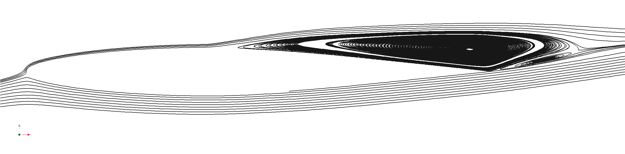
Figure 4: Airfoil NACA 64A010, $Re=2.0\times 10^{6}$, $M=0.75$, angle of attack $\alpha=6.2^{\circ}$. Streamlines showing the large separation induced by the shock obtained from the Navier-Stokes solutions.

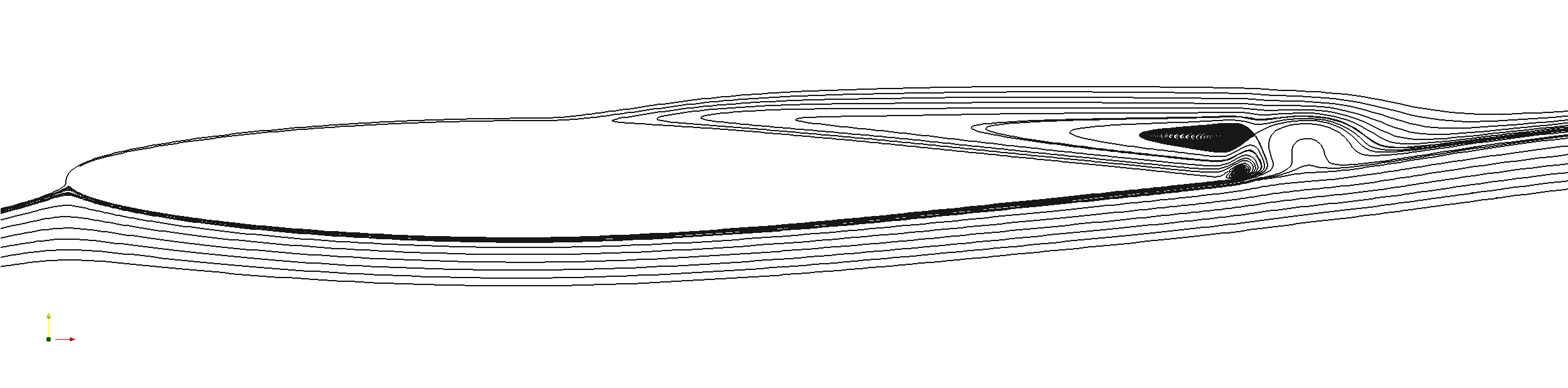
Figure 5: Airfoil NACA 64A010, $Re=2.0\times 10^{6}$, $M=0.75$, angle of attack $\alpha=6.2^{\circ}$. Streamlines showing the large separation induced by the shock obtained from the the Navier-Stokes (lhs) and GKS (rhs) solutions. Details of streamlines around the trailing edge.

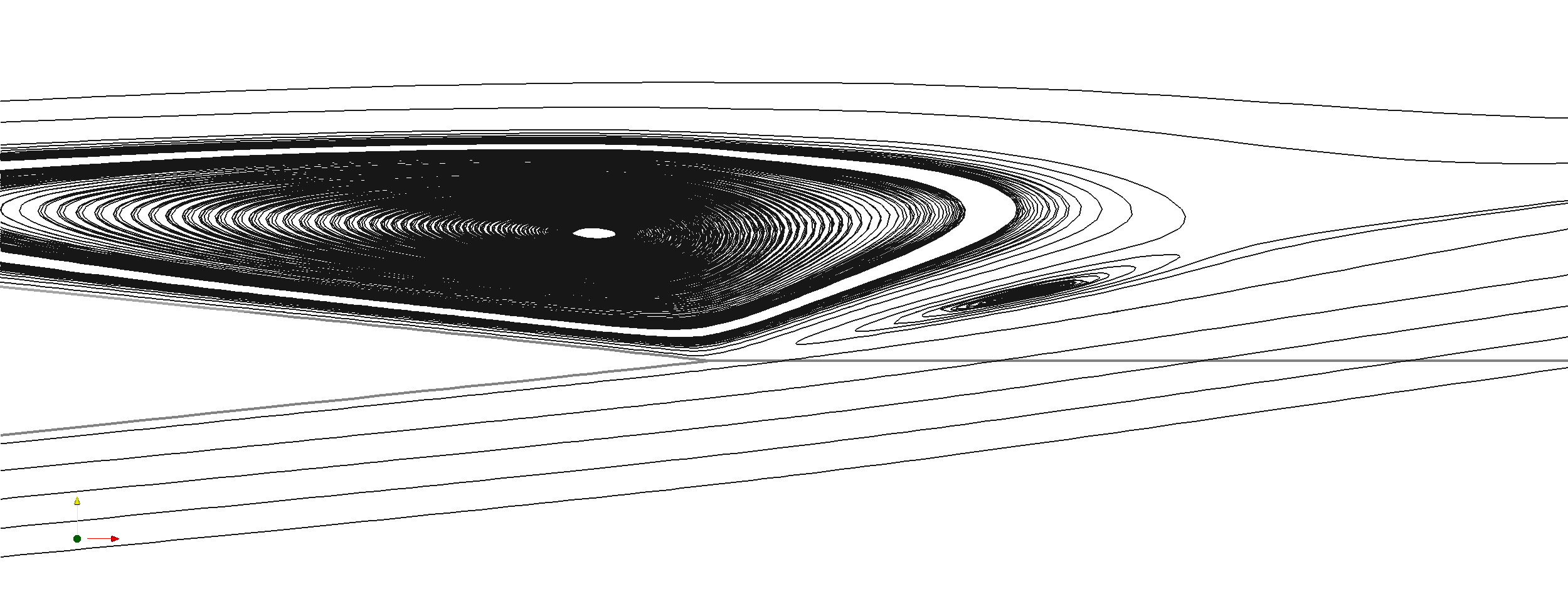
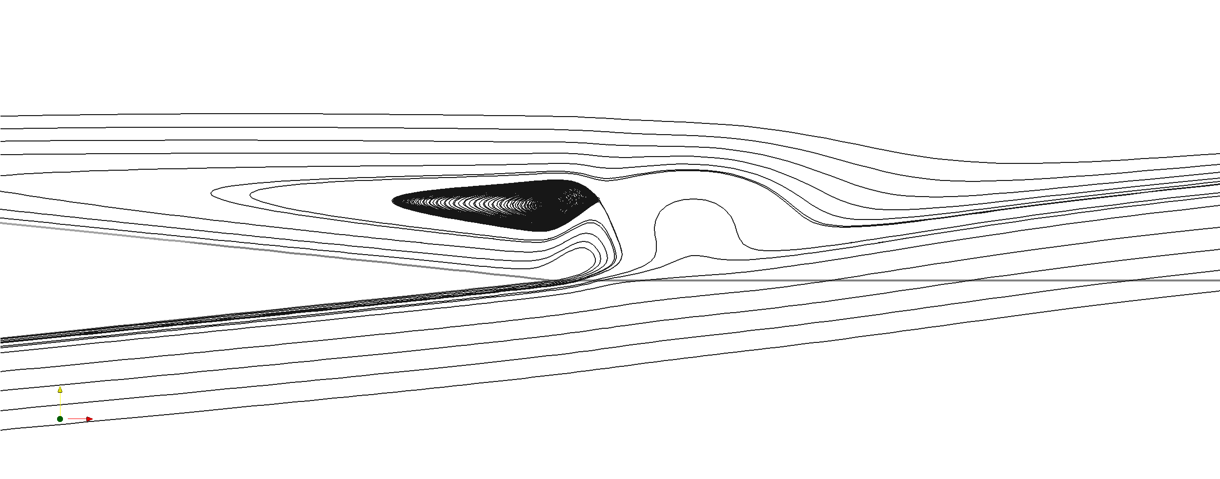
Figure 6: Airfoil NACA 64A010, $Re=2.0\times 10^{6}$, $M=0.75$, angle of attack $\alpha=6.2^{\circ}$. Streamlines showing the detail of the secondary flow around the trailing edge, obtained from the GKS solution.

5 Conclusions

The GKS investigated in this study ([19]) provides two main advantages with respect to ordinary Navier-Stokes schemes: higher-order fluxes and simultaneous treatment of transport and collisions. In the numerical experiments described, the GKS has in fact outperformed a Navier-Stokes scheme in a number of flow cases, characterized by interaction between shock and turbulent boundary layer. Interestingly, the resolution of secondary flows suggests that the GKS treats turbulence in a way similar to higher-order turbulence models (e.g. [17]), which are based on assumptions on the type of turbulence.

The turbulent GKS seem to be a good candidate to investigate turbulent flow and the more so in the rarefied / transition regime, such as for instance flow cases related to hypersonic flight, where ordinary schemes still fail to provide accurate and reliable results ([15, 14]). Not only are GKS much better suited than Navier-Stokes schemes to handle flows with not negligible $Kn$, but they would also provide advantages in turbulence modelling. It is worth reminding that virtually all turbulence theories have been developed under the assumption that the turbulent timescales are much bigger than molecular ones. As a matter of fact, in a flow characterized by $M=10$ and $Kn=0.001$ the two timescales might be comparable, i.e. $\tau_{t}\simeq\tau$. This means that ordinary Navier-Stokes schemes not only separate transport and collisions but they also miss the interactions between molecular and turbulent dynamics.

Even in the continuum regime the properties of GKS schemes are much less known than those of Navier-Stokes schemes: many aspects of GKS still need to be clarified and future activities might include the sensitivity of results to the type of turbulence model, reconstruction order and truncation order in the Chapman-Enskog expansion.

References

- [1] P.L. Bhatnagar, E.P. Gross, and M. Krook. A model for collision processes in gases. i. small amplitude processes in charged and neutral one-component systems. Physical review, 94(3):511, 1954.
- [2] C. Cercignani. The Boltzmann equation and its applications, volume 67. Springer, 1988.
- [3] H. Chen, S. Kandasamy, S. Orszag, R. Shock, S. Succi, and V. Yakhot. Extended boltzmann kinetic equation for turbulent flows. Science, 301(5633):633–636, 2003.
- [4] H. Chen, S.A. Orszag, I. Staroselsky, and S. Succi. Expanded analogy between boltzmann kinetic theory of fluids and turbulence. Journal of Fluid Mechanics, 519(1):301–314, 2004.
- [5] S.Y. Chou and D. Baganoff. Kinetic flux–vector splitting for the navier–stokes equations. Journal of Computational Physics, 130(2):217–230, 1997.
- [6] PH Cook, MA McDonald, and MCP Firman. Aerofoil rae 2822–pressure distributions, and boundary layer andwake measurements. experimental data base for computer program assessment. AGARD Advisory, 1979.
- [7] S.K. Godunov. A difference method for numerical calculation of discontinuous solutions of the equations of hydrodynamics. Matematicheskii Sbornik, 89(3):271–306, 1959.
- [8] C.D. Harris. Two-dimensional aerodynamic characteristics of the naca 0012 airfoil in the langley 8 foot transonic pressure tunnel. NASA Technical Memorandum, 1981.
- [9] A. Jameson. Solution of the euler equations for two dimensional transonic flow by a multigrid method. Applied Mathematics and Computation, 13(3-4):327–356, 1983.
- [10] DA Johnson, WD Bachalo, and FK Owen. Transonic flow past a symmetrical airfoil at high angle of attack. NASA Technical Memorandum, 1981.
- [11] JC Mandal and SM Deshpande. Kinetic flux vector splitting for euler equations. Computers & fluids, 23(2):447–478, 1994.
- [12] G. May, B. Srinivasan, and A. Jameson. An improved gas-kinetic bgk finite-volume method for three-dimensional transonic flow. Journal of Computational Physics, 220(2):856–878, 2007.
- [13] S.B. Pope. Turbulent flows. Cambridge Univ Pr, 2000.
- [14] C.J. Roy and F.G. Blottner. Review and assessment of turbulence models for hypersonic flows: 2d/axisymmetric cases. AIAA Paper, 713:2006, 2006.
- [15] CL Rumsey. Compressibility considerations for kappa-omega turbulence models in hypersonic boundary layer applications. NASA Technical Memorandum, 2009.
- [16] L. Tang. Progress in gas-kinetic upwind schemes for the solution of euler/navier-stokes equations i. overview. Computers & Fluids, 2011.
- [17] S. Wallin and A.V. Johansson. An explicit algebraic reynolds stress model for incompressible and compressible turbulent flows. Journal of Fluid Mechanics, 403:89–132, 2000.
- [18] D. C. Wilcox. Turbulence Modeling for CFD, 3rd edition. DCW Industries, Inc., La Canada CA, 2006.
- [19] K. Xu. A gas-kinetic bgk scheme for the navier–stokes equations and its connection with artificial dissipation and godunov method. Journal of Computational Physics, 171(1):289–335, 2001.
- [20] K. Xu, M. Mao, and L. Tang. A multidimensional gas-kinetic bgk scheme for hypersonic viscous flow. Journal of Computational Physics, 203(2):405–421, 2005.
- [21] K. Xu and K.H. Prendergast. Numerical navier-stokes solutions from gas kinetic theory. Journal of Computational Physics, 114(1):9–17, 1994.
- [22] S. Yoon and A. Jameson. Lower-upper symmetric-gauss-seidel method for the euler and navier-stokes equations. AIAA journal, 26(9):1025–1026, 1988.