Instantaneous frequency and amplitude of complex signals based on quaternion Fourier transform

Abstract

The ideas of instantaneous amplitude and phase are well understood for signals with real-valued samples, based on the analytic signal which is a complex signal with one-sided Fourier transform. We extend these ideas to signals with complex-valued samples, using a quaternion-valued equivalent of the analytic signal obtained from a one-sided quaternion Fourier transform which we refer to as the hypercomplex representation of the complex signal. We present the necessary properties of the quaternion Fourier transform, particularly its symmetries in the frequency domain and formulae for convolution and the quaternion Fourier transform of the Hilbert transform. The hypercomplex representation may be interpreted as an ordered pair of complex signals or as a quaternion signal. We discuss its derivation and properties and show that its quaternion Fourier transform is one-sided. It is shown how to derive from the hypercomplex representation a complex envelope and a phase.

A classical result in the case of real signals is that an amplitude modulated signal may be analysed into its envelope and carrier using the analytic signal provided that the modulating signal has frequency content not overlapping with that of the carrier. We show that this idea extends to the complex case, provided that the complex signal modulates an orthonormal complex exponential. Orthonormal complex modulation can be represented mathematically by a polar representation of quaternions previously derived by the authors. As in the classical case, there is a restriction of non-overlapping frequency content between the modulating complex signal and the orthonormal complex exponential. We show that, under these conditions, modulation in the time domain is equivalent to a frequency shift in the quaternion Fourier domain. Examples are presented to demonstrate these concepts.

1 Introduction

The instantaneous amplitude and phase of a real-valued signal have been understood since 1948 from the work of Ville [1] and Gabor [2] based on the analytic signal. A critical discussion of instantaneous amplitude and phase was given by Picinbono in 1997, particularly with reference to amplitude and phase modulation [3, §V]. The analytic signal and its associated modulation concepts can be simply described, even though a full theoretical treatment is quite deep. Given a real-valued signal $f(t)$, the corresponding analytic signal $a(t)$ is a complex signal with real part equal to $f(t)$ and imaginary part orthogonal to $f(t)$. The imaginary part is sometimes known as the quadrature signal – in the case where $f(t)$ is a sinusoid, the imaginary part of the analytic signal is in quadrature, that is with a phase difference of $-\pi/2$. The orthogonal signal is related to $f(t)$ by the Hilbert transform [4, 5]. The analytic signal has the interesting property that its modulus $|a(t)|$ is an envelope of the signal $f(t)$. The envelope is also known as the instantaneous amplitude. Thus if $f(t)$ is an amplitude-modulated sinusoid, the envelope $|a(t)|$, subject to certain conditions on the frequency content, is the modulating signal. The argument of the analytic signal, $\angle\,a(t)$ is known as the instantaneous phase and its derivative is known as the instantaneous frequency. The analytic signal has a further very interesting property: it has a one-sided Fourier transform. Thus a simple method for constructing the analytic signal (algebraically or numerically) is to compute the Fourier transform of $f(t)$, multiply the Fourier transform by a unit step which is zero for negative frequencies, and then construct the inverse Fourier transform of the resulting spectrum.

In this paper we extend the above ideas to signals with complex-valued samples. We show that if a quaternion Fourier transform is computed from a complex-valued signal, and negative frequencies in the frequency domain representation are suppressed, the inverse quaternion Fourier transform gives an equivalent of the analytic signal, which we refer to in this paper as a hypercomplex representation of the complex signal. Just as the classical analytic signal represents a real-valued signal by a complex signal (that is with a pair of real signals), the hypercomplex representation presented here represents a complex-valued signal by a quaternion signal (that is with a pair of complex signals, based on the Cayley-Dickson form of a quaternion).

We consider signals with complex-valued samples in a most general sense, without any restrictions on the relationship between the real and imaginary parts. However, we exclude the special case of an analytic signal (where the real and imaginary parts are orthogonal) because it does not possess an interesting hypercomplex representation: the two additional quaternion components of the hypercomplex representation are simply copies of the two original components. The case where the real and imaginary parts are correlated in some statistical sense is called improper, whereas an analytic signal is proper. It has been customary to handle such signals by using an augmented representation consisting of a vector containing the signal and its conjugate [6]. Recently, Lilly and Olhede [7] have published a paper on bivariate analytic signal concepts. Their approach is linked to a specific signal model, the modulated elliptical signal, which they illustrate with the example of a drifting oceanographic float, and they utilise pairs of analytic signals derived from the pair of real signals representing the time-varying positional coordinates of a drifting float. In this paper a different approach, using hypercomplex representation, is considered because it is more suited to the analysis of modulation, and also because we have at our disposal the existing tools of quaternion Fourier transforms, which provide a natural fit with modulation of a complex signal by a complex signal, for reasons which should be evident later in the paper. Note that, in essence, the approach proposed in this paper is inspired by the work of Bülow [8, 9] and Labunets [10] who considered Clifford Fourier transforms (quaternion in the case of Bülow) to process multidimensional signals. While Bülow considered 2D signals (images), here we consider 1D signals with 2D samples (complex valued samples). We are not focusing on any particular application in this paper, rather we propose a new approach to the processing of complex valued signals (including proper and improper signals, even though proper signals are well-described using the classical complex Fourier transform — they are a special case.) Schreier and Scharf’s book gives examples of applications [6].

The idea of amplitude modulation is extended to the case where the modulating signal is complex, and the ‘carrier’ is an orthonormal complex exponential, that is a complex exponential which is in a complex plane orthogonal to the complex plane of the modulating signal – this concept is easily realised using quaternions, since quaternion algebra has a 4-dimensional basis with three mutually orthogonal imaginary units. Subject to the same restrictions on frequency content as in the real-valued case, amplitude modulation in the time domain corresponds to a frequency shift in the Fourier domain. Further, a complex envelope of the hypercomplex representation can be defined which recovers the complex modulating signal. This is the complex instantaneous amplitude. Further, the phase of the orthonormal complex exponential may be recovered. This is the instantaneous phase, and its derivative is the instantaneous frequency. In the case of modulation of a complex exponential the instantaneous frequency is that of the complex exponential ‘carrier’. Just as the classical complex analytic signal contains both the original real signal (in the real part) and a real orthogonal signal (in the imaginary part), our hypercomplex signal representation contains two complex signals: the original signal and an orthogonal signal.

We have previously published partial results on this topic [11, 12, 13] as we developed the ideas presented here. The idea of orthonormal complex modulation has not previously been presented.

The sequence of topics in the rest of the paper is as follows. Section 2 presents the quaternion algebra and quaternion Fourier transform concepts used to construct the hypercomplex representation of a complex signal using a one-sided quaternion spectrum. Section 3 discusses the hypercomplex representation of a complex signal. Section 4 discusses the instantaneous amplitude and frequency concept for a complex signal through its hypercomplex representation. Section 5 presents some signal examples to illustrate the ideas presented in the paper.

2 Quaternion Fourier
Transform

In this section, we present the definition and properties of the Quaternion Fourier transform (QFT) of complex valued signals. Before introducing the main definitions, we give some prerequisites on quaternions. Interested readers may refer to [14, 15] for a more detailed presentation of quaternions.

2.1 Preliminary remarks

Quaternions were discovered by Sir W. R. Hamilton in 1843 [14]. Quaternions are 4D hypercomplex numbers that form a noncommutative division ring denoted ${\mathbb{H}}$. A quaternion $q\in{\mathbb{H}}$ has a Cartesian form: $q=q_{0}+q_{1}\boldsymbol{i}+q_{2}\boldsymbol{j}+q_{3}\boldsymbol{k}$, with $q_{0},q_{1},q_{2},q_{3}\in{\mathbb{R}}$ and $\boldsymbol{i},\boldsymbol{j},\boldsymbol{k}$ roots of $-1$ satisfying $\boldsymbol{i}^{2}=\boldsymbol{j}^{2}=\boldsymbol{k}^{2}=\boldsymbol{i}\boldsymbol{j}\boldsymbol{k}=-1$. The scalar part of $q$ is $a$: ${\cal S}(q)=q_{0}$. The vector part of $q$ is: ${\cal V}(q)=q-{\cal S}(q)$. We will also make use of the real and imaginary parts using the following notation:

$$q_{0}=\Re(q),\quad q_{1}=\Im_{\boldsymbol{i}}(q),\quad q_{2}=\Im_{\boldsymbol{j}}(q),\quad q_{3}=\Im_{\boldsymbol{k}}(q)$$ (1)

Quaternion multiplication is not commutative, so that in general $qp\neq pq$ for $p,q\in{\mathbb{H}}$. The conjugate of $q$ is $\overline{q}=q_{0}-q_{1}\boldsymbol{i}-q_{2}\boldsymbol{j}-q_{3}\boldsymbol{k}$. The norm of $q$ is $||q||=|q|^{2}=(q_{0}^{2}+q_{1}^{2}+q_{2}^{2}+q_{3}^{2})=q\overline{q}$. A quaternion with $q_{0}=0$ is called pure. $|q|$ is the modulus of $q$. If $|q|=1$, then $q$ is called a unit quaternion. The inverse of $q$ is $q^{-1}=\overline{q}/||q||$. Pure unit quaternions are special quaternions, among which are $\boldsymbol{i}$, $\boldsymbol{j}$ and $\boldsymbol{k}$. Together with the identity of ${\mathbb{H}}$, they form a quaternion basis: $\left\{1,\boldsymbol{i},\boldsymbol{j},\boldsymbol{k}\right\}$.

In ${\mathbb{H}}$, in addition to the conjugation, there exist anti-involutions which play an important role, as noticed by Bülow et al. [9]. In the special case where $\left\{1,\boldsymbol{i},\boldsymbol{j},\boldsymbol{k}\right\}$ is chosen as the basis for ${\mathbb{H}}$ these involutions are, for a given quaternion $q$, the following

$$\begin{array}[]{ccc}\overline{q}^{\boldsymbol{i}}=-\boldsymbol{i}q\boldsymbol{i},&\overline{q}^{\boldsymbol{j}}=-\boldsymbol{j}q\boldsymbol{j},&\overline{q}^{\boldsymbol{k}}=-\boldsymbol{k}q\boldsymbol{k}.\end{array}$$ (2)

Quaternions can also be viewed as complex numbers with complex components, i.e. one can write $q=z_{1}+z_{2}\boldsymbol{j}$ in the basis $\left\{1,\boldsymbol{i},\boldsymbol{j},\boldsymbol{k}\right\}$ with $z_{1},z_{2}\in{\mathbb{C}}^{\boldsymbol{i}}$, i.e. $z_{\alpha}=\Re(z_{\alpha})+\boldsymbol{i}\Im(z_{\alpha})$ for $\alpha=1,2$. This is called the Cayley-Dickson form of $q$.

Among the possible representations of $q$, we will make use in this paper of one that was recently introduced: the polar Cayley-Dickson form [16]. Any quaternion $q$ also has a unique polar Cayley-Dickson form given by:

$$q=A_{q}\exp(B_{q}\boldsymbol{j})=(a_{0}+a_{1}\boldsymbol{i})\exp((b_{0}+b_{1}\boldsymbol{i})\boldsymbol{j})$$ (3)

where $A_{q}=a_{0}+a_{1}\boldsymbol{i}$ is the complex modulus of $q$ and $B_{q}=b_{0}+b_{1}\boldsymbol{i}$ its complex phase. As explained in [16], given a degenerate quaternion $p=(c+d\boldsymbol{i})\boldsymbol{j}$, then its exponential $e^{p}$ is given by:

$$e^{p}=\cos|p|+\frac{p}{|p|}\sin|p|=\alpha+\beta\boldsymbol{j}+\delta\boldsymbol{k}$$ (4)

leading to $\alpha=\cos|p|$, $\beta=(c/|p|)\sin|p|$ and $\delta=(d/|p|)\sin|p|$, with $|p|=\sqrt{c^{2}+d^{2}}$. Recall also that, for any quaternion $p$, $|e^{p}|=1$. Then, for any quaternion $q$ given in its polar form as in equation (3):

$$e^{B_{q}\boldsymbol{j}}=\cos|B_{q}|+\boldsymbol{j}\frac{b_{0}}{|B_{q}|}\sin|B_{q}|+\boldsymbol{k}\frac{b_{1}}{|B_{q}|}\sin|B_{q}|$$ (5)

where $|B_{q}|=\sqrt{b_{0}^{2}+b_{1}^{2}}$. As a consequence, using the right hand side expression in (3), given a quaternion $q=q_{0}+q_{1}\boldsymbol{i}+q_{2}\boldsymbol{j}+q_{3}\boldsymbol{k}$, then the complex components of its polar Cayley-Dickson form, i.e. $A_{q}$ and $B_{q}$, are given as follows:

$$\left\{\begin{array}[]{rcl}A_{q}&=&\frac{q_{0}+\boldsymbol{i}q_{1}}{\cos(\sqrt{q_{2}^{2}+q_{3}^{2}})}\\ B_{q}&=&K\left(\frac{q_{0}q_{3}+q_{1}q_{2}}{q_{0}^{2}+q_{1}^{2}}+\boldsymbol{i}\frac{q_{0}q_{3}-q_{1}q_{2}}{q_{0}^{2}+q_{1}^{2}}\right)\end{array}\right.$$ (6)

with $K=\sqrt{q_{2}^{2}+q_{3}^{2}}\arctan\left(\sqrt{q_{2}^{2}+q_{3}^{2}}\right)$. In Section 4, we will make use of the complex modulus $A_{q}$ for the interpretation of the hypercomplex representation.

2.2 Quaternion Fourier transform

In this paper, we use a 1D version of the (right) QFT first defined in discrete-time form in [17]. Thus, it is necessary to specify the axis (a pure unit quaternion) of the transform. So, we will denote by $QFT_{\boldsymbol{\mu}}{\,}$ a QFT with transformation axis $\boldsymbol{\mu}$. In order to work with the classical quaternion basis $\left\{1,\boldsymbol{i},\boldsymbol{j},\boldsymbol{k}\right\}$ and for reasons that will be explained later, we will use $\boldsymbol{j}$ as the transform axis. The only restriction on the transform axis is that it must be orthogonal to the original basis of the signal (here $\left\{1,\boldsymbol{i}\right\}$). We now present the definition and some properties of the transform used here.

Definition 1.

Given a complex valued signal $z(t)=z_{r}(t)+\boldsymbol{i}z_{i}(t)$ that belongs to $L^{1}({\mathbb{R}},{\mathbb{C}})\cap L^{2}({\mathbb{R}},{\mathbb{C}})$, then the quaternion valued function denoted $Z_{\boldsymbol{j}}(\nu)$, and given as:

$$Z_{\boldsymbol{j}}(\nu)=QFT_{\boldsymbol{j}}\left[z(t)\right]=\int\limits_{-\infty}^{+\infty}z(t)e^{-\boldsymbol{j}2\pi\nu t}\mathrm{d}t$$ (7)

and with $Z_{\boldsymbol{j}}(\nu)\in L^{1}({\mathbb{R}},{\mathbb{H}})\cap L^{2}({\mathbb{R}},{\mathbb{H}})$ is called the Quaternion Fourier Transform $QFT_{\boldsymbol{j}}$ with respect to axis $\boldsymbol{j}$ of $z(t)$.

The inverse transform is defined as follows.

Definition 2.

Given a quaternion Fourier transform $Z_{\boldsymbol{j}}(\nu)$ (with respect to axis $\boldsymbol{j}$), then:

$$z(t)=IQFT_{\boldsymbol{j}}\left[Z_{\boldsymbol{j}}(\nu)\right]=\int\limits_{-\infty}^{+\infty}Z_{\boldsymbol{j}}(\nu)e^{\boldsymbol{j}2\pi\nu t}d\nu$$ (8)

is the Inverse Quaternion Fourier Transform $IQFT_{\boldsymbol{j}}$ with respect to ${\boldsymbol{j}}$ of $Z_{\boldsymbol{j}}(\nu)$.

2.3 Properties of the QFT

In order to provide insight into the advantages of using the QFT to analyze complex signals, we present a non-exhaustive list of the QFT properties.

Property 1.

(Transform symmetry) Given a complex signal $z(t)=z_{r}(t)+\boldsymbol{i}z_{i}(t)$ and its quaternion Fourier transform denoted by $Z_{\boldsymbol{j}}(\nu)$, then the following properties hold:

• The even part of $z_{r}(t)$ is in $\Re(Z_{\boldsymbol{j}}(\nu))$

• The odd  part of $z_{r}(t)$ is in $\Im_{\boldsymbol{j}}(Z_{\boldsymbol{j}}(\nu))$

• The even part of $z_{i}(t)$ is in $\Im_{\boldsymbol{i}}(Z_{\boldsymbol{j}}(\nu))$

• The odd  part of $z_{i}(t)$ is in $\Im_{\boldsymbol{k}}(Z_{\boldsymbol{j}}(\nu))$

Proof.

Expand (7) into real and imaginary parts with respect to $\boldsymbol{i}$, and expand the quaternion exponential into cosine and sine components:

$$Z_{\boldsymbol{j}}(\nu) =\!\int\limits_{-\infty}^{+\infty}{\!\left[z_{r}(t)+\boldsymbol{i}z_{i}(t)\right]}\left[\cos(2\pi\nu t)-\boldsymbol{j}\sin(2\pi\nu t)\right]\mathrm{d}t$$

$$=\!\int\limits_{-\infty}^{+\infty}\!z_{r}(t)\cos(2\pi\nu t)\mathrm{d}t-\boldsymbol{j}\!\int\limits_{-\infty}^{+\infty}\!z_{r}(t)\sin(2\pi\nu t)\mathrm{d}t$$

$$+\boldsymbol{i}\!\int\limits_{-\infty}^{+\infty}\!z_{i}(t)\cos(2\pi\nu t)\mathrm{d}t-\boldsymbol{k}\!\int\limits_{-\infty}^{+\infty}\!z_{i}(t)\sin(2\pi\nu t)\mathrm{d}t$$

from which the stated properties are evident. ∎

It is a known fact that the classical Fourier transform of a real signal possesses Hermitian symmetry. It is also known that the classical Fourier transform of a complex signal possesses no symmetry at all. The QFT of a complex signal has symmetry according to the following properties:

Property 2.

($\boldsymbol{i}$-involution reversal) Given a complex valued signal $z(t)$ and its quaternion Fourier transform denoted $QFT_{\boldsymbol{j}}[z(t)]=Z_{\boldsymbol{j}}(\nu)$, then the following property holds:

$$Z_{\boldsymbol{j}}(-\nu)=-\boldsymbol{i}Z_{\boldsymbol{j}}(\nu)\boldsymbol{i}=\overline{Z_{\boldsymbol{j}}(\nu)}^{\boldsymbol{i}}$$ (9)

Proof.

This can be directly checked from Property 1. ∎

Figure 1: Symmetry of the four components of the quaternion valued Fourier transform $Z_{\boldsymbol{j}}(\nu)$ of a complex signal $z(t)$.

This symmetry property of the QFT of a complex signal is illustrated in Figure 1 and is central to the justification of using the QFT to analyze a complex-valued signal carrying complementary but different information in its real and imaginary parts. Using the QFT, it is possible to keep the odd and even parts of the real and imaginary parts of the signal in four different components in the transform domain. This idea was also the initial motivation of Bülow, Sommer and Felsberg when they developed the monogenic signal for images [8, 9, 18]. Note that the use of hypercomplex Fourier transforms was originally introduced in 2D Nuclear Magnetic Resonance image analysis [19, 20].

For use later in the paper, we mention another property.

Property 3.

($\boldsymbol{j}$-involution conjugation) Given a complex signal $z(t)$ and its $QFT_{\boldsymbol{j}}$ denoted $Z_{\boldsymbol{j}}(\nu)$, then the $QFT_{\boldsymbol{j}}$ of its conjugate ${z^{\star}}(t)$ is given by:

$$QFT_{\boldsymbol{j}}\left[{z^{\star}}(t)\right]=-\boldsymbol{j}Z_{\boldsymbol{j}}(\nu)\boldsymbol{j}=\overline{Z_{\boldsymbol{j}}(\nu)}^{\boldsymbol{j}}$$ (10)

Proof.

This can be directly checked by calculation. ∎

An important issue for the forthcoming study of complex signals is the way modulation affects the QFT. Of special importance is ortho-complex modulation.

Property 4.

(Ortho-complex modulation) Given a complex signal $z(t)$ and its $QFT_{\boldsymbol{j}}$ denoted $Z_{\boldsymbol{j}}(\nu)$, the $QFT_{\boldsymbol{j}}$ of the ortho-complex modulation of $z(t)$ by the quaternion-valued exponential $\exp(\boldsymbol{j}2\pi\nu_{0}t)$ is

$$QFT_{\boldsymbol{j}}[z(t)e^{\boldsymbol{j}2\pi\nu_{0}t}]=Z_{\boldsymbol{j}}(\nu-\nu_{0})$$ (11)

Proof.

As $e^{\boldsymbol{j}2\pi\nu_{0}t}$ is an exponential with the same axis $\boldsymbol{j}$ as the $QFT_{\boldsymbol{j}}$, then direct calculation similar to the complex case can be performed as $e^{\boldsymbol{j}a}e^{\boldsymbol{j}b}=e^{\boldsymbol{j}(a+b)}$. The desired result is then directly obtained. ∎

Note that a similar frequency shift occurs simultaneously in the four components of the quaternion valued Fourier transform. Note also that the axis of the modulation plays an important role as a modulation using axis $\boldsymbol{i}$ or $\boldsymbol{k}$ would not lead to a simple shift of the spectrum. Also, it is obvious from this property and the convolution property (see equation 12) fulfilled by the $QFT_{\boldsymbol{j}}$ that $QFT_{\boldsymbol{j}}[e^{\boldsymbol{j}2\pi\nu_{0}t}]=\delta(\nu-\nu_{0})$.

Figure 2: Four components of the quaternion valued Fourier transform $Z_{\boldsymbol{j}}(\nu-\nu_{0})$ of the orthocomplex modulated signal $z(t)e^{\boldsymbol{j}2\pi\nu_{0}t}$ and where the complex signal $z(t)$ has a $QFT_{\boldsymbol{j}}$ verifying $\left|Z_{\boldsymbol{j}}(\nu)\right|=0$ for $\left|\nu\right|>\nu_{0}$. This spectrum is an example of (11).

Property 5.

(Positive spectra modulation) Given a complex signal $z(t)$ with a band-limited $QFT_{\boldsymbol{j}}$: $X_{\boldsymbol{j}}(\nu)=0$ for $|\nu|>\nu_{m}$ for a given $\nu_{m}$. Then, for some $\nu_{0}>\nu_{m}$, the ortho-complex modulated signal $z(t)e^{\boldsymbol{j}2\pi\nu_{0}t}$ has a right-sided $QFT_{\boldsymbol{j}}$.

Proof.

This results follows directly from property 4 and the band-limited property of $z(t)$. ∎

This property is illustrated in Figure 2.

Now, we introduce the convolution property in the case where one of the signals is real valued. Note that we do not give the general case as only the above mentioned one will be of use in the sequel.

Property 6.

(Convolution) Given $g$ and $f$ such that: $g:{\mathbb{R}}\rightarrow{\mathbb{C}}$ and $f:{\mathbb{R}}\rightarrow{\mathbb{R}}$, the $\operatorname{QFT}_{\boldsymbol{j}}$ of their convolution product $(g*f)(t)$ is:

$$QFT_{\boldsymbol{j}}\left[(g*f)(t)\right]=QFT_{\boldsymbol{j}}\left[g(t)\right]\,QFT_{\boldsymbol{j}}\left[f(t)\right]$$ (12)

Proof.

Taking the $\operatorname{QFT}_{\boldsymbol{j}}$ of their convolution product one gets the result shown in (13)

$$QFT_{\boldsymbol{j}}\left[(g*f)(t)\right] =\int\limits_{-\infty}^{+\infty}\int\limits_{-\infty}^{+\infty}g(\tau)f(t-\tau)\mathrm{d}\tau\,e^{-2\boldsymbol{j}\pi\nu t}\mathrm{d}t$$ (13)

$$=\int\limits_{-\infty}^{+\infty}g(\tau)e^{-2\boldsymbol{j}\pi\nu\tau}\mathrm{d}\tau\int\limits_{-\infty}^{+\infty}f(t^{\prime})e^{-2\boldsymbol{j}\pi\nu t^{\prime}}\mathrm{d}t^{\prime}$$

$$=QFT_{\boldsymbol{j}}\left[g(t)\right]QFT_{\boldsymbol{j}}\left[f(t)\right]$$

 

which is true thanks to the fact that $f(t)$ commutes with the $\boldsymbol{j}$ exponential as $f(t)$ is real valued. ∎

Note that the order matters in the product of the $QFT_{\boldsymbol{j}}$s in (12) as they are quaternion and complex valued (which do not commute in the general case). This expression is thus valid only when $f$ is convolved on the right. Convolution on the left would result in the appearance of a conjugation in the Fourier domain.

2.4 Hilbert transform

The quaternion Fourier transform of the Hilbert transformer $x(t)=1/\pi t$ is $-\boldsymbol{j}\operatorname{sign}(\nu)$, where $\boldsymbol{j}$ is the axis of the transform. This arises simply from the fact that using the exponential with axis $\boldsymbol{j}$ in the transform will lead to a real and $\Im_{\boldsymbol{j}}$ part for the $QFT_{\boldsymbol{j}}$ only, which is a degenerate quaternion isomorphic to a complex number. Substituting $x(t)$ into (7), we get:

$$QFT_{\boldsymbol{j}}\left[\frac{1}{\pi t}\right]=\frac{1}{\pi}\int\limits_{-\infty}^{+\infty}\frac{e^{-\boldsymbol{j}2\pi\nu t}}{t}\,\mathrm{d}t$$

and this is clearly isomorphic to the classical complex case. The solution in the classical case is $-{\boldsymbol{i}}\operatorname{sign}(\nu)$, and hence in the quaternion case must be as stated above.

It is straightforward to see that, given an arbitrary real signal $y(t)$, subject only to the constraint that its classical Hilbert transform $\mathcal{H}\left[y(t)\right]$ exists, then one can easily show that the classical Hilbert transform of the signal may be obtained using a quaternion Fourier transform as follows:

$$\mathcal{H}\left[y(t)\right]=IQFT_{\boldsymbol{j}}\left[-\boldsymbol{j}\operatorname{sign}(\nu)Y_{\boldsymbol{j}}(\nu)\right]$$ (14)

where $Y_{\boldsymbol{j}}(\nu)=QFT_{\boldsymbol{j}}\left[y(t)\right]$. This result follows from the isomorphism between the quaternion and complex Fourier transforms when operating on a real signal, and it may be seen to be the result of a convolution between the signal $y(t)$ and the quaternion Fourier transform of $x(t)=1/\pi t$. Note that $\boldsymbol{j}$ and $Y_{\boldsymbol{j}}(\nu)$ commute as a consequence of $y(t)$ being real. We can now define the Hilbert transform of a complex signal.

Definition 3.

Consider a complex signal $z(t)=z_{r}(t)+\boldsymbol{i}z_{i}(t)$ and its quaternion Fourier transform $Z_{\boldsymbol{j}}(\nu)$ as defined in Definition 1. Then, the hypercomplex analogue of the Hilbert transform of $z(t)$, is as follows:

$$\mathcal{H}_{\boldsymbol{j}}\left[z(t)\right]=\mathcal{F}_{\boldsymbol{j}}^{-1}\left[-\boldsymbol{j}\operatorname{sign}(\nu)Z_{\boldsymbol{j}}\right](\nu)$$ (15)

where the Hilbert transform is thought of as: $\mathcal{H}_{\boldsymbol{j}}\left[z(t)\right]=p.v.\left(z*\frac{1}{\pi t}\right)$, where the principal value (p.v.) is understood in its classical way. This result follows from (14) and the linearity of the quaternion Fourier transform. To extract the imaginary part, the vector part of the quaternion signal must be multiplied by $-\boldsymbol{i}$. An alternative is to take the scalar or inner product of the vector part with $\boldsymbol{i}$. Note that $\boldsymbol{j}$ and $Z_{\boldsymbol{j}}(\nu)$ anticommute because $\boldsymbol{j}$ is orthogonal to $\boldsymbol{i}$, the axis of $Z_{\boldsymbol{j}}(\nu)$. Therefore the ordering is not arbitrary, but changing it simply conjugates the result.

Note that the signal $z(t)$ is considered to be non-analytic in the classical (complex) sense, that is its real and imaginary parts are not orthogonal. However, this definition is valid if $z(t)$ is analytic, as it can be considered as a degenerate case of the more general non-analytic case. We end this section with a useful property of the right-sided $QFT_{\boldsymbol{j}}$.

Property 7.

(Positive spectrum quaternion signal) Consider a $QFT_{\boldsymbol{j}}$ denoted by $Z_{\boldsymbol{j}}(\nu)$. Then, $Z_{\boldsymbol{j}}(\nu)$ is said to be right-sided if $Z_{\boldsymbol{j}}(\nu)=0$, $\forall\nu<0$. Now, if a $QFT_{\boldsymbol{j}}$ denoted $Z_{\boldsymbol{j}}(\nu)$ is right-sided, then its Inverse Quaternion Fourier transform $IQFT_{\boldsymbol{j}}\left[Z_{\boldsymbol{j}}(\nu)\right]$ is a quaternion valued signal.

Proof.

The $QFT_{\boldsymbol{j}}$ of a complex signal has the symmetry described in Property 2 and illustrated in Figure 1. Assuming these symmetries, a right-sided $QFT_{\boldsymbol{j}}$ can only be obtained from a $QFT_{\boldsymbol{j}}$, denoted $Z_{\boldsymbol{j}}(\nu)$, by the following linear combination: $(1+\operatorname{sign}(\nu))Z_{\boldsymbol{j}}(\nu)$ which simply cancels out the negative frequencies. Now, the $IQFT_{\boldsymbol{j}}$ of $\operatorname{sign}(\nu)$ is, as previously seen, equal to $\boldsymbol{j}/\pi t$. The convolution of $1/\pi t$ with $z(t)$ leads to a complex signal with $\Re$ and $\Im_{\boldsymbol{i}}$ which, when multiplied by $\boldsymbol{j}$ becomes a degenerate quaternion signal with only the $\Im_{\boldsymbol{j}}$ and $\Im_{\boldsymbol{k}}$ parts non-zero. Now, the total $IQFT_{\boldsymbol{j}}$ of $(1+\operatorname{sign}(\nu))Z_{\boldsymbol{j}}(\nu)$ consists of $z(t)+{\boldsymbol{j}}\left(\frac{1}{\pi t}*z(t)\right)(t)$ which is thus made of a real part and three imaginary parts of axis ${\boldsymbol{i}}$, ${\boldsymbol{j}}$ and ${\boldsymbol{k}}$. ∎

In the next section, we make use of the QFT and Hilbert transform to build up a hypercomplex representation for complex valued signals.

3 The hypercomplex signal
representation

We define a hypercomplex representation, denoted $\hat{z}(t)$, of the complex signal $z(t)$ by a similar approach to that originally developed by Ville [1]. The $\hat{z}(t)$ signal is quaternion-valued. The following definitions give the details of the construction of this signal.

Property 8.

(Hypercomplex extension) Given a complex signal $z(t)$, one can associate to it a unique canonical pair corresponding to a (complex) modulus and phase. The modulus and phase are uniquely defined through the hypercomplex representation of the complex signal, which is quaternion valued.

Proof.

Cancelling the negative frequencies of the QFT leads to a quaternion signal in the time domain. Then, any quaternion signal has a modulus and phase defined using its CD polar form. ∎

Definition 4.

Given a complex valued signal $z(t)$ that can be expressed as $z(t)=z_{r}(t)+\boldsymbol{i}z_{i}(t)$, then the hypercomplex representation of $z(t)$, denoted $\hat{z}(t)$ is given by:

$$\hat{z}(t)=z(t)+\boldsymbol{j}\mathcal{H}_{\boldsymbol{j}}\left[z(t)\right]$$ (16)

where $\mathcal{H}_{\boldsymbol{j}}\left[z(t)\right]$ is the hypercomplex analogue of the Hilbert transform of $z(t)$ defined in the preceding definition. The $QFT_{\boldsymbol{j}}$ of this hypercomplex representation of the complex signal, denoted $\hat{Z}_{\boldsymbol{j}}(\nu)$, is thus:

$$\hat{Z}_{\boldsymbol{j}}(\nu) =Z_{\boldsymbol{j}}(\nu)-\boldsymbol{j}^{2}\operatorname{sign}(\nu)Z_{\boldsymbol{j}}(\nu)$$

$$=\left[1+\operatorname{sign}(\nu)\right]Z_{\boldsymbol{j}}(\nu)$$

$$=2U(\nu)Z_{\boldsymbol{j}}(\nu)$$

where $U(\nu)$ is the classical unit step function.

This result is unique to the quaternion Fourier transform representation of the hypercomplex representation, which has a one-sided quaternion Fourier spectrum. This means that the hypercomplex representation may be constructed from a complex signal $z(t)$ in exactly the same way that an analytic signal may be constructed from a real signal, by suppression of negative frequencies in the Fourier domain. The only difference is that in the hypercomplex representation, a quaternion rather than a complex Fourier transform must be used, and of course the complex signal must be put in the form $z(t)=z_{r}(t)+\boldsymbol{i}z_{i}(t)$ which, although a quaternion signal, is isomorphic to the original complex signal.

Property 9.

(Hypercomplex phasor form) Given a complex signal $z(t)$, one can associate to it a unique canonical pair $\left[\rho(t),\phi(t)\right]$ consisting of a modulus and a phase. The modulus and phase are uniquely defined through the hypercomplex representation of the complex signal.

Proof.

Cancelling the negative frequencies of the $QFT_{\boldsymbol{j}}$ of a complex signal leads to a quaternion signal in the time domain, with similar frequency content (the original $QFT_{\boldsymbol{j}}$ of the complex signal can be recovered thanks to the symmetry properties of the quaternion Fourier transform). As any quaternion signal has a unique modulus and phase defined through its CD polar form, those are uniquely associated to the original complex signal. ∎

A second important property of the hypercomplex representation of a complex signal $z(t)$ is that it maintains a separation between the different even and odd parts of the original signal.

Property 10.

(Orthogonal split) The original signal $z(t)$ is the simplex part [22, Theorem 1], [23, § 13.1.3] of its corresponding hypercomplex representation $\hat{z}(t)$. The perplex part is the orthogonal or ‘quadrature’ component, $o(t)$. They are obtained by:

$$z(t) =\frac{1}{2}\left(\hat{z}(t)+\overline{\hat{z}(t)}^{\boldsymbol{i}}\right)$$ (17)

$$o(t) =\frac{1}{2}\left(z_{+}(t)-\overline{\hat{z}(t)}^{\boldsymbol{i}}\right)$$ (18)

Proof.

This follows from (16). Writing this in full by substituting the orthogonal signal for $\mathcal{H}_{\boldsymbol{j}}\left[z(t)\right]$:

$$\hat{z}(t)=z(t)+\boldsymbol{j}o(t)=z_{r}(t)+\boldsymbol{i}z_{i}(t)+\boldsymbol{j}o_{r}(t)-\boldsymbol{k}o_{i}(t)$$

and substituting this into equation (17), we get:

$$z(t) =\frac{1}{2}\left(\begin{aligned} &\phantom{\boldsymbol{i}\left[\right.}z_{r}(t)+\boldsymbol{i}z_{i}(t)+\boldsymbol{j}o_{r}(t)-\boldsymbol{k}o_{i}(t)\\ -&\boldsymbol{i}\left[z_{r}(t)+\boldsymbol{i}z_{i}(t)+\boldsymbol{j}o_{r}(t)-\boldsymbol{k}o_{i}(t)\right]\boldsymbol{i}\end{aligned}\right)$$

and since $$\boldsymbol{i} \boldsymbol{j} \boldsymbol{i}\boldsymbol{j}=-\boldsymbol{j}\boldsymbol{i}$$ and are orthogonal unit pure quaternions, :

$$=\frac{1}{2}\left(\begin{aligned} &\phantom{\boldsymbol{i}\left[\right.}z_{r}(t)+\boldsymbol{i}z_{i}(t)+\boldsymbol{j}o_{r}(t)-\boldsymbol{k}o_{i}(t)\\ +&\phantom{\boldsymbol{i}\left[\right.}z_{r}(t)+\boldsymbol{i}z_{i}(t)-\boldsymbol{j}o_{r}(t)+\boldsymbol{k}o_{i}(t)\end{aligned}\right)$$

from which the first part of the result follows. Equation (18) differs only in the sign of the second term, and it is straightforward to see that if $\hat{z}(t)$ is substituted, $z(t)$ cancels out, leaving $o(t)$. ∎

4 Instantaneous amplitude,
phase and frequency

Using the hypercomplex representation $\hat{z}(t)$ of a complex signal $z(t)$, we now investigate the concept of instantaneous amplitude and phase for $z(t)$.

Recall that $\hat{z}(t)$ is quaternion valued, and thus it can be expressed using its polar Cayley-Dickson form given in (3) as:

$$\hat{z}(t)=\hat{\rho}(t)e^{\hat{\phi}(t)\boldsymbol{j}}$$ (19)

where $\hat{\rho}(t)$ is called the instantaneous amplitude of $\hat{z}(t)$ and $\hat{\phi}(t)$ is the instantaneous phase of $\hat{z}(t)$. The pair $\left[\hat{\rho}(t),\hat{\phi}(t)\right]$ is canonical and associated to $z(t)$. The one-to-one correspondence between $z(t)$ and the canonical pair can be demonstrated using the same arguments used by Picinbono in [3]. Indeed, as presented in the previous sections, $\hat{z}(t)$ has a one-sided spectrum. This ensures the spectral characterization (see [3, II.B]) of the canonical pair. In addition, the one-to-one correspondence is ensured because $e^{\boldsymbol{j}\hat{\phi}(t)}$ is a phase signal with respect to the $QFT_{\boldsymbol{j}}$. Now, just as explained in [3, III], $e^{\boldsymbol{j}\hat{\phi}(t)}$ is a unimodular signal, and in order for it to be one-sided, some restrictions apply to $\hat{\phi}(t)$. In short, the phase $\hat{\phi}(t)$ is of the form:

$$\hat{\phi}(t)=\theta+2\pi\nu_{0}t+\hat{\phi}_{b}(t)$$ (20)

where $\theta$ is a constant, $\nu_{0}$ is a given frequency and $\hat{\phi}_{b}(t)$ is a band-limited contribution with maximum frequency $B>\nu_{0}$. In Section 5, we present examples of the former two terms.

With all these considerations, one can state the following.

Definition 5.

Given a complex signal $z(t)$, its instantaneous amplitude $\hat{\rho}(t)$ and instantaneous phase $\hat{\phi}(t)$ are obtained through the polar Cayley-Dickson form of its hypercomplex representation $\hat{z}(t)$.

As noted above, through this definition, $\left[\hat{\rho}(t),\hat{\phi}(t)\right]$ is a canonical pair associated to $z(t)$. Note that, unlike in the classical case of the analytic signal associated to a real signal, the instantaneous amplitude of $z(t)$ is complex valued. However, it represents the low-frequency part (non modulated) of $z(t)$. The instantaneous frequency can now be defined similar to the classical case.

Definition 6.

The instantaneous frequency of the complex signal $z(t)$ is defined as:

$$\hat{f}(t)=\frac{1}{2\pi}\frac{d\hat{\phi}(t)}{dt}$$ (21)

where $\hat{\phi}(t)$ is the instantaneous phase of $z(t)$.

Like the classical case, this definition follows naturally from the Taylor series for $\hat{\phi}(t)$ about $t_{0}$, namely,

$$\hat{\phi}(t) =\hat{\phi}(t_{0})+(t-t_{0})\frac{d\hat{\phi}(t_{0})}{dt}+R$$

$$=(\hat{\phi}(t_{0})-t_{0}\frac{d\hat{\phi}(t_{0})}{dt})+\frac{d\hat{\phi}(t_{0})}{dt}t+R$$

where $R$ is small when $t$ is close to $t_{0}$ and we see that $\frac{d\hat{\phi}(t_{0})}{dt}$ has the role of frequency. Unlike the classical case, the complex nature of $z(t)$ requires that the oscillation direction evolves over time (as can be seen for example in Figure 3 and 9). Information on the orientation of this oscillation, i.e. the osculating plane orientation, can be recovered from the instantaneous amplitude $\hat{\rho}(t)$. More precisely, the normal to the osculating plane, denoted $\hat{n}(t)$, is:

$$\hat{n}(t)=\hat{\rho}(t)\times\hat{\rho}^{\prime}(t)$$ (22)

where $\hat{\rho}^{\prime}(t)=d\hat{\rho}(t)/dt$ and where $\times$ is the cross product of vectors corresponding to the time-varying complex signals: $[z_{r}(t)~{},~{}z_{i}(t)~{},~{}t]$ is the vector associated with the complex signal $z(t)=z_{r}(t)+\boldsymbol{i}z_{i}(t)$. From a geometric point of view, $\hat{\rho}^{\prime}(t)$ can be considered as the velocity of $z(t)$.

Such a geometrical description of a complex signal can be achieved with the use of concepts defined through the $QFT_{\boldsymbol{j}}$. Such an analysis could be developed to higher dimensional signals using geometric algebra Fourier transforms.

5 Examples

We present three examples in which a band-limited complex signal $A(t)$ modulates an orthogonal complex exponential $\exp(B(t)\boldsymbol{j})$. This can be represented using the polar Cayley-Dickson form of (3) as:

$$q(t)=A(t)\exp(B(t)\boldsymbol{j})$$ (23)

The result is a quaternion-valued signal. We can extract from this, two complex signals using the Cartesian Cayley-Dickson form: $q(t)=z(t)+o(t)\boldsymbol{j}$, where $z(t)=z_{r}(t)+z_{i}(t)\boldsymbol{i}$ and similarly for $o(t)$. In what follows we take the first of these to be our modulated complex signal (the second is a type of ‘quadrature’ signal).

In the first example, the orthonormal complex exponential has constant frequency, so that simply:

$$B_{1}(t)=2\pi\nu_{0}t$$ (24)

where $\nu_{0}$ is an arbitrary constant value. This example can be generated in the frequency domain, since the modulation in the time domain corresponds to a shift in the frequency domain by $\nu_{0}$. The complex signal is $z_{1}(t)$.

In the second example, $B_{2}(t)$ is a step function of the form:

$$B_{2}(t)=\left\{\begin{array}[]{lcr}2\pi\nu_{0}t&\text{if}&\hfill t\in[0,0.25]\\ 2\pi\nu_{1}t&\text{if}&\hfill t\in[0.25,0.75]\\ 2\pi\nu_{0}t&\text{if}&\hfill t\in[0.75,1]\par\end{array}\right.$$ (25)

where $\nu_{0}$ and $\nu_{1}$ are arbitrary constant values. This example is generated in the same manner as the first one. The complex signal is thus $z_{2}(t)$ for this example.

In the third example, the frequency of the complex exponential sweeps linearly from an initial value to double the initial value and back to the initial value. That is:

$$B_{3}(t)=\alpha(\Pi_{T/2}*\Pi_{T/2})(t-T/2)$$ (26)

where $\Pi$ is the boxcar function with $T=0.5$ and $\alpha$ a constant in the present case. This example is also generated in the time domain. The complex signal is denoted $z_{3}(t)$.

We present in the sequel how the modulating complex signal, and the frequency of the carrier can be recovered from the quaternion hypercomplex representation of the complex signal using the instantaneous amplitude (the ‘envelope’) and the instantaneous phase, both of which are computed from the Cayley-Dickson polar form of the quaternion-valued hypercomplex representation of the complex signals $z_{1}(t)$, $z_{2}(t)$ and $z_{3}(t)$.

Figure 3 shows a modulated complex signal $z_{1}(t)$ (in blue) constructed by modulating an orthonormal complex exponential with a band-limited complex signal. The latter was constructed from a pseudo-random signal by filtering in the frequency domain to suppress all frequencies higher than an upper limit of 16 cycles over the length of the signal. The orthocomplex exponential in this case has constant frequency four times that of the highest frequency of the baseband complex signal, and the modulated signal was created by frequency shifting the quaternion Fourier transform of the baseband signal, as in (11). The complex envelope $\hat{\rho}_{1}(t)$ of the hypercomplex representation of $z_{1}(t)$, i.e. $\hat{z}_{1}(t)$, is displayed in black in Figure 3.

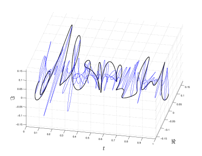
Figure 3: Band-limited signal $z_{1}(t)$ (blue) and envelope $\hat{\rho}_{1}(t)$ (black) of the hypercomplex representation $\hat{z}_{1}(t)$ associated to $z_{1}(t)$.

Figure 4 shows the instantaneous phase $\hat{\phi}_{1}(t)$ of the hypercomplex representation $\hat{z}_{1}(t)$ of the signal $z_{1}(t)$ displayed in Figure 3. This phase is obtained using the polar Cayley-Dickson phase of the hypercomplex representation $\hat{z}_{1}(t)$.

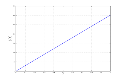
Figure 4: Phase $\hat{\phi}_{1}(t)$ recovered from the polar Cayley-Dickson form of the hypercomplex representation $\hat{z}_{1}(t)$ of the signal $z_{1}(t)$ displayed in Figure 3, showing the linearly increasing phase $B_{1}(t)$.

In the second example, the orthocomplex exponential is again constant, but this time ‘by parts’, with two different constant values taken over the time period considered, as expressed in (25). The initial frequency of the exponential is 12.5 times that of the highest frequency of the baseband complex signal, and it then doubles at time $0.25$ before returning to its original value at time $0.75$. Figure 5 shows the modulated signal in this case.

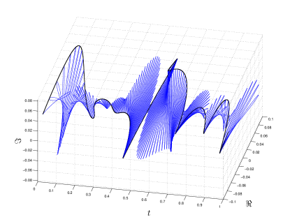
Figure 5: Band-limited signal $z_{2}(t)$ (blue) envelope $\hat{\rho}_{2}(t)$ (black) of the hypercomplex representation $\hat{z}_{2}(t)$ associated to $z_{2}(t)$.

The recovered envelope $\hat{\rho}_{2}(t)$ is exactly as in the previous example, the frequency changes in the complex exponential makes no difference to the recovery of the envelope. The polar Cayley-Dickson phase $\hat{\phi}_{2}(t)$ is plotted in Figure 6 after unwrapping.

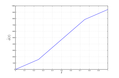
Figure 6: Phase $\hat{\phi}_{2}(t)$ recovered from the polar Cayley-Dickson form of the hypercomplex representation $\hat{z}_{2}(t)$ of the signal $z_{2}(t)$ in Figure 5, after unwrapping.

For this second example, we also present two zoomed views, Figures 7 and 8, taken for two different time intervals. On these two figures, in addition to the original signal $z_{2}(t)$ and the envelope $\hat{\rho}_{2}(t)$, some local geometric information is displayed. At several times, the vectors $\hat{\rho}_{2}^{\prime}(t)$ (blue) and $\hat{n}_{2}(t)$ (red) are displayed. One can identify that $\hat{\rho}^{\prime}_{2}(t)$ is the vector tangent to the envelope $\hat{\rho}_{2}(t)$ of the signal $z_{2}(t)$, while the vector $\hat{n}_{2}(t)$ is normal to the osculating plane. This local information gives access to the plane in which the signal is ‘oscillating’ over time. Note that this geometric information has been obtained from attributes derived from the hypercomplex representation of the original signal $z_{2}(t)$, i.e. through simple spectral considerations. Such geometric quantities are classically obtained from 3D curves using the Frenet-Serret formulae [24, Chap. I] for example.

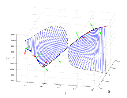
Figure 7: Original signal $z_{2}(t)$ (blue) and complex envelope $\rho_{2}(t)$(black) of the orthocomplex modulation 5 for the time period: $t=0.3$ to $t=0.6$. For different times, the tangent vectors (blue), normal (red) and binormal (green) are displayed. The blue vectors represent $\hat{\rho}_{2}^{\prime}(t)$ for some given $t$, the tangent to the complex envelope. Green vectors represent $\hat{n}_{2}(t)$ (given in (22)), i.e. the normal to the instantaneous osculating plane of the signal $z_{2}(t)$.

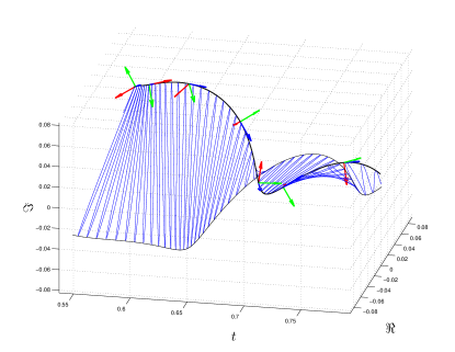
Figure 8: Original signal $z_{2}(t)$ (blue) and complex envelope $\rho_{2}(t)$(black) of the orthocomplex modulation 5 for the time period: $t=0.55$ to $t=0.8$. For different times, the tangent vectors (blue), normal (red) and binormal (green) are displayed. The blue vectors represent $\hat{\rho}_{2}^{\prime}(t)$ for some given $t$, the tangent to the complex envelope. Green vectors represent $\hat{n}_{2}(t)$ (given in (22)), i.e. the normal to the instantaneous osculating plane of the signal $z_{2}(t)$.

In the third example, the orthocomplex exponential has a much higher frequency than the baseband signal (which is the same signal as in the first example). The initial frequency of the exponential is 25 times that of the highest frequency of the baseband complex signal, and it sweeps linearly to double the initial frequency, and then back down to the initial value. The original signal $z_{3}(t)$ together with the complex envelope $\hat{\rho}_{3}(t)$ of the hypercomplex representation $\hat{z}_{3}(t)$ are displayed in Figure 9. In Figure 10, we present the instantaneous frequency $\hat{\phi}_{3}^{\prime}(t)$ obtained from $\hat{z}_{3}(t)$. The linearity of the chirp frequency behaviour is recovered (singularity at time $0.5$ is due to the behaviour of the phase at this point) as expected.

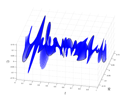
Figure 9: Band-limited signal $z_{3}(t)$ (blue) envelope $\hat{\rho}_{3}(t)$ (black) of the hypercomplex representation $\hat{z}_{3}(t)$ associated to $z_{3}(t)$.

Figure 10: Instantaneous frequency $\hat{\phi}_{3}^{\prime}(t)$ obtained from the hypercomplex representation $\hat{z}_{3}(t)$ of the complex signal $z_{3}(t)$.

Note that the notion of instantaneous frequency that we have introduced here for complex signals is indeed very similar to the notion of angular velocity that is well known in physics. The analogy is possible thanks to the fact that the knowledge of $\hat{n}(t)$ gives access to the time-varying orientation of the 2D plane in which the signal is oscillating.

Finally, a short-time quaternion Fourier transform (STQFT) of the modulated signal $z_{3}(t)$ is shown in Figure 11, showing the frequency sweep of the orthocomplex exponential.

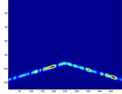
Figure 11: Time-frequency depiction of the modulated signal $z_{3}(t)$ in Figure 9. The figure shows the modulus of a short-time quaternion Fourier transform with window length 128.

The modulus of the STQFT is real valued and it shows the frequency content evolution over time for $z_{3}(t)$. The values for which the STQFT modulus vanishes represent the moment when the complex envelope vanishes.

Notice that we have not illustrated the case where $B_{q}(t)$ is complex. This is because it is the modulus of $B_{q}(t)$ which is the phase in the orthocomplex exponential, and a complex $B_{q}(t)$ would need to have a modulus representing phase. It is not clear what the argument would represent. A constant frequency is represented by a linearly increasing real phase, that is $B_{q}(t)$ would be a real-valued ramp.

As can be seen from (5), if $B_{q}(t)$ is real, that is $B_{q}(t)=b_{o}(t)$, we have the following form for the modulated signal, where $A_{q}(t)=a_{0}(t)+a_{1}(t)\boldsymbol{i}$:

$$q(t) =A_{q}(t)\left[\cos|b_{0}(t)|+\sin|B_{0}(t)|\boldsymbol{j}\right]$$ (27)

$$=A_{q}(t)\cos|b_{0}(t)|+A_{q}(t)\sin|B_{0}(t)|\boldsymbol{j}$$

This quaternion signal contains $A_{q}(t)$ modulated by a cosine in the first Cayley-Dickson component (the first two components of the quaternion), and $A_{q}(t)$ modulated by a sine in the second Cayley-Dickson component (the third and fourth components of the quaternion). The orthonormal formulation using quaternions achieves the following:

• The ‘carrier’ is modeled by a complex exponential, rather than a trigonometric function, giving the usual advantages of the notation.

• Because the quadrature component is orthogonal to the in-phase component, the two are separated in the signal and in the Fourier domain.

These advantages disappear if we replace $\boldsymbol{j}$ with $\boldsymbol{i}$ and revert to complex algebra, because then the in-phase and quadrature components become mixed in a single complex signal, rather than being kept separate in the components of a quaternion signal. In complex algebra we can represent a complex exponential modulated by a real signal, or a real ‘carrier’, represented by a trigonometric function, modulated by a complex signal. We cannot represent a complex signal modulating a complex exponential.

6 Conclusions

We have shown in this paper how the classical concepts of instantaneous amplitude and phase may be extended to the case of complex signals using a quaternion hypercomplex representation of a complex signal. We have also shown that the classical case of amplitude modulation can be extended to the complex case provided that we maintain an orthogonal separation between the complex plane of the modulating signal, and the complex plane of the complex exponential ‘carrier’, and maintain a separation in frequency between the modulating signal and the ‘carrier’ exactly as in the classical case. The orthogonal separation required is easily realised using a quaternion representation, and we can then compute a hypercomplex representation of the complex signal using a suitable quaternion Fourier transform. This hypercomplex representation of the signal preserves symmetries that would be lost using a complex Fourier transform. It is analogous to the classical analytic signal.

We have shown that the quaternion polar representation permits us to recover from the hypercomplex representation, both the instantaneous amplitude and the instantaneous phase. From the instantaneous phase, it is also possible to recover the instantaneous frequency as well as the osculating plane that gives geometric information about the direction in which the signal is oscillating.

As quaternions are isomorphic to the geometric Clifford algebra $Cl(0,2)$ of ${\mathbb{R}}^{2}$, it is evident from our results that there are possibilities to extend the work presented here to the case of vector-valued signals where the samples are $N$-dimensional, by using Clifford Fourier transforms in $2^{N}$ dimensions.

References

- [1] J. Ville, Théorie et applications de la notion de signal analytique, Cables et Transmission 2A (1948) 61–74.
- [2] D. Gabor, Theory of communication, Journal of the Institution of Electrical Engineers 93 (26) (1946) 429–457, part III.
- [3] B. Picinbono, On instantaneous amplitude and phase of signals, IEEE Trans. Signal Process. 45 (3) (1997) 552–560.
- [4] S. L. Hahn, Hilbert transforms in signal processing, Artech House signal processing library, Artech House,, Boston, Mass.; London, 1996.
- [5] S. L. Hahn, Hilbert transforms, in: A. D. Poularikas (Ed.), The transforms and applications handbook, CRC Press, Boca Raton, 1996, Ch. 7, pp. 463–629, a CRC handbook published in cooperation with IEEE press.
- [6] P. J. Schreier, L. L. Scharf, Statistical signal processing of complex-valued data: the theory of improper and noncircular signals, Cambridge University Press, 2010.
- [7] J. M. Lilly, S. C. Olhede, Bivariate instantaneous frequency and bandwidth, IEEE Trans. Signal Process. 58 (2) (2010) 591–603. doi:10.1109/TSP.2009.2031729.
- [8] T. Bülow, Hypercomplex spectral signal representations for the processing and analysis of images, Ph.D. thesis, University of Kiel, Germany (1999).
- [9] T. Bülow, G. Sommer, Hypercomplex signals – a novel extension of the analytic signal to the multidimensional case, IEEE Trans. Signal Process. 49 (11) (2001) 2844–2852. doi:10.1109/78.960432.
- [10] E. Rundblad-Labunets, V. Labunets, Spatial-color Clifford algebras for invariant image recognition, in: G. Sommer (Ed.), Geometric computing with Clifford algebras, Springer, 2001, Ch. 7, pp. 155–185.
- [11] S. J. Sangwine, N. Le Bihan, Hypercomplex analytic signals: Extension of the analytic signal concept to complex signals, in: Proceedings of EUSIPCO 2007, 15th European Signal Processing Conference, European Association for Signal Processing, Poznan, Poland, 2007, pp. 621–4.
- [12] N. Le Bihan, S. J. Sangwine, The H-analytic signal, in: Proceedings of EUSIPCO 2008, 16th European Signal Processing Conference, European Association for Signal Processing, Lausanne, Switzerland, 2008, pp. 5 pp.
- [13] N. Le Bihan, S. J. Sangwine, About the extension of the 1D analytic signal to improper complex valued signals, in: Eighth International Conference on Mathematics in Signal Processing, The Royal Agricultural College, Cirencester, UK, 2008, p. 45.
- [14] W. R. Hamilton, Lectures on Quaternions, Hodges and Smith, Dublin, 1853, available online at Cornell University Library: http://mathematics.library.cornell.edu/.
- [15] J. P. Ward, Quaternions and Cayley Numbers: Algebra and Applications, Vol. 403 of Mathematics and Its Applications, Kluwer, Dordrecht, 1997.
- [16] S. J. Sangwine, N. Le Bihan, Quaternion polar representation with a complex modulus and complex argument inspired by the Cayley-Dickson form, Advances in Applied Clifford Algebras 20 (1) (2010) 111–120, published online 22 August 2008. doi:10.1007/s00006-008-0128-1.
- [17] S. J. Sangwine, T. A. Ell, The discrete Fourier transform of a colour image, in: J. M. Blackledge, M. J. Turner (Eds.), Image Processing II Mathematical Methods, Algorithms and Applications, Horwood Publishing for Institute of Mathematics and its Applications, Chichester, 2000, pp. 430–441, proceedings Second IMA Conference on Image Processing, De Montfort University, Leicester, UK, September 1998.
- [18] M. Felsberg, G. Sommer, The monogenic signal, IEEE Trans. Signal Process. 49 (12) (2001) 3136–3144.
- [19] R. Ernst, G. Bodenhausen, A. Wokaun, Principles of nuclear magnetic resonance in one and two dimensions, Oxford University Press, 1987.
- [20] M. A. Delsuc, Spectral representation of 2D NMR spectra by hypercomplex numbers, Journal of magnetic resonance 77 (1988) 119–124.
- [21] G. Chirikjian, A. Kyatkin, Engineering applications of noncommutative harmonic analysis, CRC Press, 2000.
- [22] T. A. Ell, S. J. Sangwine, Hypercomplex Wiener-Khintchine theorem with application to color image correlation, in: IEEE International Conference on Image Processing (ICIP 2000), Vol. II, Institute of Electrical and Electronics Engineers, Vancouver, Canada, 2000, pp. 792–795. doi:10.1109/ICIP.2000.899828.
- [23] S. J. Sangwine, T. A. Ell, N. Le Bihan, Hypercomplex models and processing of vector images, in: C. Collet, J. Chanussot, K. Chehdi (Eds.), Multivariate Image Processing, Digital Signal and Image Processing Series, ISTE Ltd, and John Wiley, London, and Hoboken, NJ, 2010, Ch. 13, pp. 407–436.
- [24] M. D. Carmo, Differential Geometry of curves and surfaces, Prentice-Hall, 1976.